A Branch–and–Cut Algorithm to Design LDPC Codes without Small Cycles in Communication Systems

Abstract

In a digital communication system, information is sent from one place to another over a noisy communication channel using binary symbols (bits). Original information is encoded by adding redundant bits, which are then used by low–density parity–check (LDPC) codes to detect and correct errors that may have been introduced during transmission. Error correction capability of an LDPC code is severely degraded due to harmful structures such as small cycles in its bipartite graph representation known as Tanner graph (TG). We introduce an integer programming formulation to generate a TG for a given smallest cycle length. We propose a branch-and-cut algorithm for its solution and investigate structural properties of the problem to derive valid inequalities and variable fixing rules. We introduce a heuristic to obtain feasible solutions of the problem. Our computational experiments show that our algorithm can generate LDPC codes without small cycles in acceptable amount of time for practically relevant code lengths.

Keywords: Telecommunications, LDPC code design, integer programming, branch–and–cut algorithm.

1 Introduction and Literature Review

Telecommunication is the transmission of messages from a transmitter to a receiver over a potentially unreliable communication environment. In a digital communication system, binary code symbols (bits) represent the messages. In parallel to the rapid developments in technology, digital communication systems find several application areas: messaging via digital cellular phones, fiber optic internet, TV broadcasting or agricultural monitoring through digital satellites, and receiving high quality images of Jupiter under NASA’s Juno mission [1] are some examples of digital communication.

In practice, numerous transmitter–receiver pairs share the same communication environment such as air or space. Hence, radio waves, electrical signals, and light waves over fiber optic channels accumulate some amount of noise on the medium. The noise in the environment can cause transmission errors or failures. Channel coding is the term used for the collection of techniques that are employed in digital communications to ensure that a transmission is recovered with minimal or no errors. These techniques encode the original information by adding redundant bits. When the receiver receives information, the decoder estimates the original information by detecting and correcting errors in the received vector with the help of redundant bits.

Among the codes that are used in the decoding process at receiver, low–density parity–check (LDPC) code family has received attention thanks to its high error detection and correction capabilities. LDPC codes were first proposed by Gallager in 1962 and today they are used in wireless network standard (IEEE 802.11n), WiMax (IEEE 802.16e), and digital video broadcasting standard (DVB-S2) [2]. They have sparse parity–check matrices, i.e., $\mathbf{H}$ matrix, and can alternatively be represented by bipartite graphs known as Tanner graphs (TG) [3]. A TG (or LDPC code) is said to be (J, K)–regular if all nodes at one side of the bipartite graph have degree $J$ and all other nodes have degree $K$ (see Section 2 for a formal definition). Otherwise, a TG (or LDPC code) is irregular and degrees of the nodes can be expressed with a degree distribution.

Iterative decoding algorithms, which have low complexity and low decoding latency due to the sparsity property of parity–check matrix, have been developed on TG [4, 5]. Iterative decoding algorithms decide on whether each code symbol is 0 or 1 by calculating probabilities for the code symbols to estimate the original information. The calculated probabilities are dependent on each other if there are cycles on the TG. In order to minimize code symbol estimation errors, designing LDPC codes to maximize the smallest cycle length, i.e., $girth$, is useful. There are different approaches in the literature for obtaining a TG with large girth.

One approach is to eliminate the cycles with length smaller than the target girth from a given TG. In [6], certain edges are exchanged within TG to eliminate small cycles without simultaneously creating any others. In the edge deletion algorithm of [7], an edge that is common for the maximum number of cycles is selected. These methods are heuristic approaches and they change the degree distribution of the nodes in the TG. It is known that the degree distribution affects the error correction capability of an LDPC code [8]. Hence, it is important to eliminate as few edges from TG as possible. There are studies based on optimization techniques in the literature to find the best degree distribution of an irregular TG in terms of error correction capability [8, 9].

Another way of designing an LDPC code is to construct a TG from scratch. Bit–Filling heuristic in [10] starts with a large girth target and decreases target as it inserts edges to TG one–by–one. The heuristic terminates when a prescribed girth is met. A randomized approach in [11] can create irregular LDPC codes by introducing new edges in a zig–zag pattern. Progressive Edge Growth (PEG) heuristic in [12] is based on adding edges to the TG iteratively without constructing small cycles. PEG algorithm is adjusted to generate a regular LDPC code in [13] and an irregular LDPC code in [14] for improving the error correction performance. Independent tree–based heuristic of [15] can iteratively construct regular LDPC codes whose girth values are better than the ones obtained by PEG. A protograph is a TG with a relatively small number of nodes. Design of LDPC codes with simple protographs is investigated in [16] to obtain infinite dimensional LDPC codes. Different studies in the literature focus on the design of LDPC codes with large girth using the protograph [17, 18].

Algebraic construction is to construct structured LDPC with algebraic and combinatorial methods. Turbo LDPC (T–LDPC) codes are structured regular codes whose TG includes two trees connected by an interleaver. In [19], authors design the interleaver to avoid small cycles and obtain T–LDPC codes with high girth. Quasi–cyclic LDPC (QC–LDPC) codes consist of identity matrices whose columns are shifted by a certain amount. A method that can build QC–LDPC codes with girth at least 6 using Vandermonde matrices is introduced in [20]. A technique to generate irregular QC–LDPC codes with girth at least 8 is given in [21]. Quasi–cycle constraints are added to PEG algorithm in order to obtain regular and irregular QC–LDPC codes in [22]. Other studies also use PEG algorithm for this code family [23] – [25]. For the same code family, a lifting method is given in [26] and generalized polygones are used in [27]. Patent [28] describes a method for QC–LDPC codes, that guarantees a girth of at least 8.

The above mentioned methods are heuristic approaches and they may fail to generate a TG for a given dimension with a target girth value. On the other hand, optimization techniques are capable of finding a TG for a given girth value, or proving that there cannot be such a TG. Combinatorial approaches to design QC–LDPC codes are utilized in [29] to find the best degree distribution of the nodes in a TG. Authors obtain the degree distribution by evaluating all alternatives with respect to some performance metrics and choosing the most promising one. Then, authors construct a TG for the selected degree distribution. In [30], the selection criteria of PEG algorithm to locate an edge in a TG is modified in order to have a better girth value than PEG. The generated TG does not necessarily have the largest girth value, since their method is a TG constructive heuristic. There are other LDPC code constructive heuristics in the literature that avoid small cycles [31] – [33]. A genetic algorithm to design a TG with a small number of nodes is given in [34]. In [35] a modified shortest–path algorithm is used to construct a TG.

Our contribution to the literature can be listed as follows:

• We investigate the LDPC code design problem, which seeks a TG of desired dimension with a target girth value, from an optimization point of view.

• We propose an integer programming formulation to generate LDPC codes with a given girth value and develop a branch–and–cut algorithm for its solution.

• We investigate structural properties of the problem for $(J,K)-$regular codes to improve our algorithm by applying a variable fixing scheme, adding valid inequalities and utilizing an initial solution generation heuristic. Our computational results indicate that our proposed methods significantly improve solvability of the problem.

• We also illustrate how our method can be used to find the smallest dimension $n$ that one can generate a $(J,K)-$regular code (see Table 7).

The remainder of the paper is organized as follows: we formally define the problem and introduce our mathematical formulation in the next section. Section 3 explains the proposed branch–and–cut method and techniques to improve its performance. We test the efficiacy of our methods via computational experiments in Section 4. Some concluding remarks and comments on future work appear in Section 5.

2 Problem Definition

Figure 1 shows information flow in a digital communication system. In Figure 1, let the original information be a binary vector $\mathbf{u}=(u_{1}u_{2}...u_{k})$ of $k$–bits, i.e., $u_{i}\in\{0,1\}$. Encoder adds redundant parity–check bits to vector $\mathbf{u}$ by utilizing a $k\times n$ generator matrix $\mathbf{G}$. That is codeword $\mathbf{w}=(w_{1}w_{2}...w_{n})$ of $n$–bits, where $n\geq k$ and $w_{i}\in\{0,1\}$, is obtained through the operation $\mathbf{w}=\mathbf{uG}$. In a codeword $\mathbf{w}$, there are $k$ information bits and $(n-k)$ parity–check bits, which are used to test whether there are errors in the transmission. For integrity of the communication, codeword $\mathbf{w}$ should be in the null space of the $(n-k)\times n$ parity–check matrix $\mathbf{H}$, i.e., $\mathbf{w}\mathbf{H}^{\textrm{T}}=\mathbf{0}$ (mod 2) holds.

After transmission, the receiver gets vector $\mathbf{v}$ of $n$–bits as shown in Figure 1. Decoder detects whether the received vector $\mathbf{v}$ includes errors or not by checking whether the expression $\mathbf{v}\mathbf{H}^{\textrm{T}}$ is equal to vector $\mathbf{0}$ in (mod 2) or not. In the case that $\mathbf{v}$ is erroneous, the decoder attempts to determine error locations and fix them [36]. As a result, the information $\mathbf{u}$ sent from the source is estimated as $\hat{\mathbf{u}}$ at the sink.

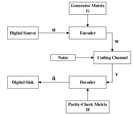
Figure 1: Digital communication system diagram

In this work, we focus on the binary symmetric channel (BSC) for modeling the noisy communication channel. As shown in Figure 2, in a BSC, an error occurs with probability $p$ and the transmitted bit flips, i.e., if a bit is 0, it becomes 1 and vice versa. The transmission is completed without any errors with probability $1-p$ [37]. The decoder aims to find the locations of the errors in BSC. Once the decoder detects a bit is erroneous, it corrects the error by flipping the bit’s value.

Figure 2: Binary symmetric channel

LDPC codes are members of linear block codes that can be represented by a sparse parity–check matrix $\mathbf{H}$, i.e., the number of ones at every row and column of the $\mathbf{H}$ matrix is forced to be very small. An LDPC code is regular, if there are constant number of ones at each column and row of the matrix. As given in Figure 3, a $(3,6)-$regular LDPC code has only 3 ones at each column and 6 ones at each row independent from the dimension of the $\mathbf{H}$. This implies that for $(3,6)-$regular LDPC code with dimension $1500\times 3000$, only 0.2% of the matrix elements are nonzero.

$$\mathbf{H}=\begin{bmatrix}0&1&0&0&1&1&1&1&1&0\\ 0&0&0&0&1&1&1&1&1&1\\ 1&0&1&1&1&1&1&0&0&0\\ 1&1&1&1&0&0&0&0&1&1\\ 1&1&1&1&0&0&0&1&0&1\\ \end{bmatrix}$$

Figure 3: A parity–check matrix from $(3,6)-$regular LDPC code family

An LDPC code can alternatively be represented as a TG, which is a sparse bipartite graph, corresponding to the $\mathbf{H}$ matrix [3]. On one part of the TG there is a variable node $j$ ($v_{j}$), $j\in\{1,...,n\}$, for each bit of received vector. Each row of the $\mathbf{H}$ matrix represents a parity–check equation and corresponds to a check node $i$ ($c_{i}),i\in\{1,...,n-k\}$, on the other part of the TG. A check node is said to be satisfied if its parity–check equation is equal to zero in (mod 2). The degree of $v_{j}$ ($c_{i}$) is the number of adjacent check nodes (variable nodes) on the TG. Hence, $\mathbf{H}$ matrix is the bi–adjacency matrix of the TG. This representation of LDPC codes is practical due to the advantage of applying iterative decoding algorithms easily. Figure 4 shows the TG representation of the $\mathbf{H}$ matrix defined in Figure 3.

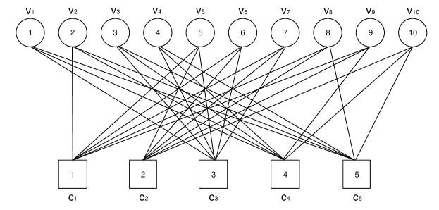
Figure 4: TG representation of the parity–check matrix given in Figure 3

It is known that iterative decoding algorithms may fail to decode in the existance of small cycles (such as $(v_{1},\ c_{3},\ v_{4},\ c_{4})$ in Figure 4) [38]. The length of a smallest cycle is known as the $girth$ of the graph [39]. In this work, we will focus on designing LDPC codes whose TGs do not contain small cycles. In particular, we aim to construct a TG with girth no smaller than a given target girth value.

3 Solution Methods

In this section, we introduce our integer programming formulations and propose a branch–and–cut algorithm for the solution of the problem. We investigate additional methods to improve the performance of our branch–and–cut algorithm. We summarize the terminology used in this paper in Table 1.

Table 1: List of symbols

Parameters
$k$	length of the original information
$n$	length of the encoded information, number of columns in $\mathbf{H}$
$m$	$n-k$, number of rows in $\mathbf{H}$
$\mathbf{G}$	generator matrix
$\mathbf{H}$	parity–check matrix
$p$	error probability in BSC
$T$	target girth
$v_{j}$	variable node $j$
$c_{i}$	check node $i$
$dv_{j}$	target degree of $v_{j}$
$dc_{i}$	target degree of $c_{i}$
$\rho(i,j)$	cycle region of $(i,j)$
Decision Variables
$X_{ij}$	$(i,j)$ entry of the $\mathbf{H}$ matrix
$dv^{s}_{j}$	slack for degree of $v_{j}$
$dc^{s}_{i}$	slack for degree of $c_{i}$

3.1 Mathematical Formulations

In our Girth Feasibility Model (GFM), our aim is to generate an $\mathbf{H}$ matrix of dimensions $(m,n)$, where $m=n-k$, with girth no smaller than a given value $T$. In the GFM model given below, $X_{ij}$ variable represents the $(i,j)$ entry of the $\mathbf{H}$ matrix, $dv_{j}$ is the degree of variable node $j$, and $dc_{i}$ is the degree of check node $i$. Constraints (2) and (3) allow generation of an irregular code with the given degree values. As a special case, one can obtain a $(J,K)-$regular $\mathbf{H}$ matrix by picking $dv_{j}=J$ for all $j$ and $dc_{i}=K$ for all $i$.

We introduce cycle breaking constraints (4) for the cycles with length less than the target girth $T$. In GFM, the objective is a constant, since the target girth $T$ is a given value. Hence, any feasible solution of the model will be optimal.

Girth Feasibility Model (GFM):

max $$\;\;T$$ (1)

s.t.: $$\sum_{i=1}^{m}X_{ij}=dv_{j},\;j=1,...,n$$ (2)

$$\sum_{j=1}^{n}X_{ij}=dc_{i},\;i=1,...,m$$ (3)

$$\sum_{(i,j)\in C}X_{ij}\leq|C|-1,\;\forall C\;\mbox{{cycle with }}|C|<T$$ (4)

$$X_{ij}\in\{0,1\},\;\;i=1,...,m,\;j=1,...,n.$$ (5)

An alternative modeling approach is to assume $dv_{j}$ and $dc_{i}$ as the target degrees of $v_{j}$ and $c_{i}$, respectively. In Minimum Degree Deviation Model (MDD), the objective is to minimize the degree deviations $dv^{s}_{j}$ of $v_{j}$ and $dc^{s}_{i}$ of $c_{i}$ from the target values.

Minimum Degree Deviation Model (MDD):

min $$\;\;\sum_{j=1}^{n}dv^{s}_{j}+\sum_{i=1}^{m}dc^{s}_{i}$$ (6)

s.t.: $$\sum_{i=1}^{m}X_{ij}+dv^{s}_{j}=dv_{j},\;j=1,...,n$$ (7)

$$\sum_{j=1}^{n}X_{ij}+dc^{s}_{i}=dc_{i},\;i=1,...,m$$ (8)

$$(\ref{cons2})-(\ref{xvar})$$ (9)

$$dv^{s}_{j},dc^{s}_{i}\geq 0,\;\;i=1,...,m,\;j=1,...,n.$$ (10)

One can observe that MDD is always feasible, since $X_{ij}=0$ for all $(i,j)$, $dv^{s}_{j}=dv_{j}$ for all $j$, and $dc^{s}_{i}=dc_{i}$ for all $i$ is a trivial solution. Moreover, if the optimum objective function value of MDD is zero, which means constraints (7) and (8) are satisfied without deviation, we get a feasible (optimum) solution of GFM.

As we explain in Proposition 3, GFM can be infeasible depending on the value of the target girth $T$. Hence, in our study, we work with the MDD model. Since there can be an exponential number of cycles in a TG, we can have exponential number of constraints (4) in the corresponding MDD model. In order to obtain a solution in an acceptable amount of time, we add the constraints (4) in a cutting–plane fashion to MDD. This gives rise to our branch–and–cut algorithm explained in the next section.

3.2 Branch–and–Cut Algorithm

The main steps of our Branch–and–Cut (BC) algorithm are listed in Algorithm 1. In the BC algorithm, we are given a target girth value $T$ and the dimensions of $\mathbf{H}$ matrix as $(m,n)$. We initialize our algorithm by relaxing constraints (4) from MDD, to obtain relaxed model $\text{MDD}^{r}$. Steps $(I.1)-(I.3)$ are our improvement techniques (see Section 3.3) to the BC algorithm.

Algorithm 1: (Branch–and–Cut) Input: Target girth value $T$, $(m,n)$ 0. Obtain $\text{MDD}^{r}$ by removing constraints (4) from MDD, set $x^{*}=null$ and $z^{*}=\infty$. $(I.1)$ Apply Algorithm 4 to fix some $X_{ij}$ variables, update $x^{*}$ and $z^{*}$. $(I.2)$ Add valid inequalities given in Proposition 5 to $\text{MDD}^{r}$. $(I.3)$ Apply Algorithm 6 to generate a feasible solution, update $x^{*}$ and $z^{*}$.        add $\text{MDD}^{r}$ to list $\mathcal{L}$. 1. While list $\mathcal{L}$ is not empty 2.      Select and remove a problem from $\mathcal{L}$. 3.      Solve LP relaxation of the problem. 4.      If the solution is infeasible, Then prune the branch and go to Step 1. 5.      Else let the current solution be $x$ with objective value $z$. 6.      End If 7.      If $z\geq z^{*}$, Then prune the branch and go to Step 1. 8.      If $x$ is an integer solution,                   If Algorithm 2 finds cycles smaller than $T$, Then add cuts (4) and go to Step 3.                   Else set $z^{*}\leftarrow z$, $x^{*}\leftarrow x$.                   End If 9.      Else If Algorithm 3 generates any cuts, Then add cuts (4) and go to Step 3. 10.    Else branch to partition the problem into subproblems.                       Add these problems to $\mathcal{L}$ and go to Step 1. 11.    End If 12. End While Output: $\mathbf{H}$ matrix with girth at least $T$

We can find either an integral or a fractional solution after solving the relaxed MDD. In the case we find an integral solution, we test its feasibility with respect to the relaxed constraints (4) with Algorithm 2. The integral solution is separated from the solution space by adding required constraints from (4) if the solution is not feasible. Similarly, we try to separate a fractional solution from the solution space with Algorithm 3, in order to strengthen the linear relaxation of MDD.

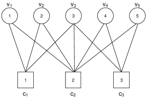
Figure 5: An example TG for Algorithm 2

In the integral solution separation problem, we find all cycles in the TG whose length is less than $T$ with a depth–first–search algorithm running in $\mathcal{O}(|V|+|E|)$ time using Algorithm 2. In Figure 6, we illustrate Algorithm 2 with $T=6$ on the TG given in Figure 5. In Figure 6a, the search algorithm starts with $v_{1}$ at level 0, i.e., $l=0$, and it is labeled. We label $c_{1}$ at $l=1$, $v_{2}$ at $l=2$ and $c_{2}$ at $l=3$, since they are the first untracked neighbors of their predecessors. At $l=4$, we visit $v_{1}$ but it has been previously labeled. This means that we have a cycle of length–4 consisting of nodes stored in $nodeTrack$ array and we add this cycle to $\mathcal{C}$ set, which keeps all cycles whose length is less than $T$ in the current integral $\mathbf{H}$ matrix.

Algorithm 2: (Integral Solution Separation) Input: A solution of $\text{MDD}^{r}$ with integral $X_{ij}$ values, $T$ target girth 1. Let set of cycles $\mathcal{C}=\emptyset$ and $nodeTrack$ be an array 2. For Each variable node $j$, let $l=1$ 3.      While $l>0$, Do set $nodeTrack[0]=j$ and label node $j$ 4.          For Each level $l$ from 1 to $T-2$ 5.              Set $nodeTrack[l]$ to first untracked neighbor of $nodeTrack[l-1]$ 6.              If $nodeTrack[l]$ is labeled, Then a cycle of length $l$ is added to $\mathcal{C}$                           unlabel $nodeTrack[l]$ and                           go to next untracked neighbor of $nodeTrack[l-1]$                           If no such neighbor, Then $l\leftarrow l-1$ 7.              Else label $nodeTrack[l]$ and $l\leftarrow l+1$, End If 8.          For Each 9.      End While 10. End For Each Output: Set of cycles $\mathcal{C}$

In Figure 6b, we consider other untracked neighbors of $c_{2}$ at level 4. After observing that none of $v_{3}$, $v_{4}$ and $v_{5}$ form a cycle, we unlabel them and return to level 3. At $l=3$, we see that there are no other untracked neighbors of $c_{2}$ and backtrack to level 2. In Figure 6c, we see $v_{3}$ is untracked and we label it at $l=2$. We label $c_{2}$ at $l=3$ and $v_{1}$ at $l=4$. This means we found another cycle of length–4 and add this to set $\mathcal{C}$.

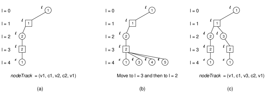
Figure 6: Depth–first–search in integral solution separation

The time to find an optimal solution of MDD can be improved by reducing the feasible region using cuts for fractional solutions. In such a case, we have fractional $X_{ij}$ values in the TG. We consider finding a maximum average cost cycle in the TG with $X_{ij}$ as cost values. If this cycle violates constraints (4) and its length is less than $T$, then we can add the corresponding violated constraint.

Minimum mean cost cycle is a well known network problem in the literature and there is a polynomial time solution algorithm for the directed graphs [40]. The problem simply aims to find a directed cycle $C$ with the smallest mean cost $\sum_{(i,j)\in C}X_{ij}/|C|$ in a graph. However, we cannot implement this algorithm directly, since a TG is undirected. For the solution, we can update best known mean cost by implementing a negative cycle detection algorithm repeatedly. Bellman–Ford algorithm can detect negative cycles while searching 1–to–many shortest paths for directed graphs. Bellman–Ford algorithm is also applicable for undirected graphs in $\mathcal{O}(|V||E|)$ time, if for an edge $(i,j)$ the algorithm updates distance label of node $j$ when it is not the predecessor of node $i$ [40]. If the algorithm detects a negative cycle, we can track the predeccessor list to form the cycle.

In the fractional solution separation problem, we use the undirected Bellman–Ford algorithm to detect negative cycles within a mean cost update method. We first set edge costs as $-X_{ij}$ to turn our maximization problem to minimization. Let $\mu$ represent an estimation on the minimum mean cost, and $\mu^{*}$ denote the (unknown) optimal value of $\mu$. Then, given a $\mu$ value, we update the edge costs to $(-X_{ij}-\mu)$ and check for the existance of a negative cycle. If we start with a $\mu$ that is an upper bound for $\mu^{*}$, we can face with one of these cases for the minimum mean cost $\mu^{*}$.

Case 1: $G$ has a negative cycle $C$. In this case, $\sum_{(i,j)\in C}(-X_{ij}-\mu)<0$. This means,

$$\mu>-\frac{\sum_{(i,j)\in C}X_{ij}}{|C|}>\mu^{*}.$$ (11)

Hence, $\mu$ is a strict upper bound on $\mu^{*}$. We can update $\mu$ as $\mu=-\frac{\sum_{(i,j)\in C}X_{ij}}{|C|}$ in the next iteration.

Case 2: $G$ has a zero–cost cycle $C^{*}$. In this case, $\sum_{(i,j)\in C^{*}}(-X_{ij}-\mu)=0$. This means,

$$\mu=-\frac{\sum_{(i,j)\in C^{*}}X_{ij}}{|C^{*}|}=\mu^{*}.$$ (12)

Hence, $\mu=\mu^{*}$ and $C^{*}$ is a minimum mean cost cycle.

Algorithm 3: (Fractional Solution Separation) Input: A solution of $\text{MDD}^{r}$ with fractional $X_{ij}$ values, $T$ target girth 1. Let $\mu=0$, set cost of edge $(i,j)$ as $(-X_{ij}-\mu)$ 2. While we can detect negative cycle $C$ with undirected Bellman–Ford 3.      If $|C|<T$ and $C$ is violating (4), Then add corresponding cut (4) 4.      Update $\mu\leftarrow-\frac{\sum_{(i,j)\in C}X_{ij}}{|C|}$ 5. End While Output: Cuts added to $\text{MDD}^{r}$ model

Fractional solution separation algorithm is summarized in Algorithm 3. We set initial $\mu=0$, since it is an upper bound on $\mu^{*}$. If we can find a negative cycle with length $|C|<T$, we can add a cut to MDD if it is violated. This means that $C$ is a cycle with $\sum_{(i,j)\in C}X_{ij}>|C|-1$. We continue updating $\mu$ values until we find a minimum mean cycle.

3.3 Improvements to the Branch–and–Cut Algorithm

In this section we propose some improvements to the BC algorithm given in the previous section. We first observe that the solution space of MDD includes symmetric solutions. Hence, we consider a variable fixing approach to decrease the adverse effect of symmetry. Secondly, we introduce some valid inequalities to improve the linear relaxation of MDD. Finally, we adapt an algorithm from the telecommunications literature, i.e., PEG, to provide an initial solution to the BC algorithm.

3.3.1 Symmetry in the MDD Solution Space

In combinatorial optimization problems such as scheduling, symmetry among the solutions is an important issue, which directly affects the performance of applied solution methods [41, 42]. We observe that the feasible region of MDD contains symmetric solutions. That is, there can be isomorphic representations of a TG by permuting the variable and check nodes. As an example, the variable nodes are in the order of $\{v_{1},v_{2},v_{3},v_{4}\}$ in Figure 7a and the names of $v_{2}$ and $v_{4}$ are swapped in Figure 7b.

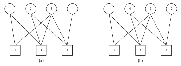
Figure 7: Symmetry in MDD solution space

In Figure 8, $\mathbf{H_{1}}$ and $\mathbf{H_{2}}$ are the parity–check matrices for TGs in Figures 7a and 7b, respectively. We see that although TGs are isomorphic, their $\mathbf{H}$ matrix representations are not identical. In the MDD solution space $\mathbf{H_{1}}$ and $\mathbf{H_{2}}$ are considered as two different solutions, which increases the complexity of the solution algorithm.

$$\mathbf{H_{1}}=\begin{bmatrix}1&0&1&0\\ 1&1&1&0\\ 0&1&1&1\\ \end{bmatrix}\hskip 28.45274pt\mathbf{H_{2}}=\begin{bmatrix}1&0&1&0\\ 1&0&1&1\\ 0&1&1&1\\ \end{bmatrix}$$

Figure 8: Parity–check matrices for the TGs in Figure 7

We can calculate the number of symmetric solutions for a TG as $(n!)(m!)$, since we can permute $n$ variable nodes as $(n!)$ and $m$ check nodes as $(m!)$ different ways.

3.3.2 Symmetry Breaking with Variable Fixing

In the literature, ordering the decision variables, adding symmetry–breaking cuts to the formulation and reformulating the problem are some of the techniques to eliminate symmetric solutions from the feasible region [42, 43]. In our case, we propose a fixing scheme for nonzero $X_{ij}$ entries of $\mathbf{H}$ matrix that breaks symmetry and does not form any cycles in TG.

In our variable fixing method (given as Algorithm 4) we consider $(J,K)$–regular $\mathbf{H}$ matrices and two modes, i.e., $basic$ and $extended$. In the $basic$ mode, we fix first $K$ entries in the first row to 1 and first $J$ entries in the first column to 1. The remaining entries in the first row and column are set to 0, since constraints (2) for $j=1$ and constraints (3) for $i=1$ are satisfied. We illustrate the $basic$ and $extended$ modes in Figure 9 for a $(3,6)-$regular code of dimensions $(30,60)$ below. Bold entries in Figure 9 are fixed with the $basic$ mode.

Algorithm 4: (Variable Fixing) Input: $(m,n)$ dimensions, $(J,K)$ values, $mode$ type 0. Let $r_{cr}=\lfloor(n-1)/(K-1)\rfloor$ and $c_{cr}=\lfloor(m-1)/(J-1)\rfloor$        Set $X_{1j}=0$, $j=1,...,n$, $X_{i1}=0$, $i=1,...,m$        If $mode=extended$            For $i=2,...,r_{cr},j=1,...,n$, set $X_{ij}=0$            For $i=r_{cr}+1,...,m,j=2,...,c_{cr}$, set $X_{ij}=0$        End If 1. Set $X_{1j}=1,j=1,...,K$ and $X_{i1}=1,i=1,...,J$ 2. If $mode=extended$ 3.      For $i=2,...,r_{cr}+1,j=1,...,K-1$, 4.          If $1+(i-1)(K-1)+j\leq n$, Then set $X_{i,1+(i-1)(K-1)+j}=1$. 5.      End For 6.      For $i=1,...,J-1,j=2,...,c_{cr}+1$, 7.          If $1+j(J-1)+i\leq m$, Then set $X_{1+j(J-1)+i,j}=1$. 8.      End For 9. End If Output: Some $X_{ij}$ values are fixed

In the $extended$ mode, we extend variable fixing further as dimensions $(m,n)$ of the $\mathbf{H}$ matrix allow. In Figure 9, the labels on the rows and colums show the sum of the values in that row and column, respectively. We observe that for $r_{cr}=\lfloor(n-1)/(K-1)\rfloor$ many rows the sum is equal to 6 and $c_{cr}=\lfloor(m-1)/(J-1)\rfloor$ many columns the sum is equal to 3. Hence, for $c_{cr}$–columns constraints (2) and for $r_{cr}$–rows constraints (3) are satisfied. We remain with a reduced rectangle of size $(m-r_{cr})\times(n-c_{cr})$, which includes the unfixed $X_{ij}$ variables shown as dots. Algorithm 4 runs in $\mathcal{O}(nc_{cr})$ time.

In practical applications, for a $(J,K)-$regular code $J<K<n$ relationship is valid. In Proposition 1, we use this relationship to compare $r_{cr}$ and $c_{cr}$.

Figure 9: Variable fixing on a $(3,6)-$regular $\mathbf{H}$ matrix of dimensions (30, 60)

Proposition 1.

Let $J<K<n$. For a $(J,K)-$regular code of dimensions $(m,n)$, $r_{cr}\leq c_{cr}$ where $r_{cr}=\lfloor(n-1)/(K-1)\rfloor$ and $c_{cr}=\lfloor(m-1)/(J-1)\rfloor$.

Proof. Let $\frac{J}{K}=a\in(0,1)$, then $mK=nJ\implies m=na$. We can write, $\frac{m-1}{J-1}=\frac{na-1}{Ka-1}=\frac{a(n-1)+a-1}{a(K-1)+a-1}>\frac{n-1}{K-1}$, since $a<1$. From here we obtain $\lfloor\frac{n-1}{K-1}\rfloor\leq\lfloor\frac{m-1}{J-1}\rfloor\implies r_{cr}\leq c_{cr}$. $\square$

In Proposition 2, we show that any $(J,K)$–regular $\mathbf{H}$ matrix of dimensions $(m,n)$ that has sufficiently large girth $T$ can be expressed as in Figure 10 by reordering its rows and columns.

Proposition 2.

Let $\mathbf{H}$ be a $(J,K)$–regular code of dimensions $(m,n)$. Let $R$ be the reduced rectangle of size $(m-r_{cr})\times(n-c_{cr})$ and $R\bigcup S$ be the region between the two extending 1–blocks as in Figure 10. Let $\rho(i,j)$ be the length of a smallest cycle that is formed when $X_{ij}=1$, and $\tau=\max_{(i,j)\in S}\{\rho(i,j)\}$.Then, nonzero entries of $\mathbf{H}$ can be represented as two extending 1–blocks as in Figure 10 by reordering its rows and columns if it has a girth $T>\tau$. Remaining nonzero entries are in the reduced rectangle $R$.

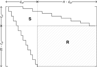
Figure 10: Reordered $(J,K)$–regular $\mathbf{H}$ matrix with girth $T>\tau$

Proof. Let $\mathbf{H}$ be $(J,K)$–regular matrix of dimensions $(m,n)$ with girth $T>\tau$. Let us apply the following reordering algorithm with time complexity $\mathcal{O}(c_{cr})$ on the $\mathbf{H}$.

Algorithm 5: (Reordering) Input: $\mathbf{H}$, $(m,n)$ dimensions, $(J,K)$ values, $T$ value 1. Pick row 1, reorder columns such that all ones are in first $K$ columns.        Pick column 1, reorder rows such that all ones are in first $J$ rows. 2. For $s\in\{2,...,r_{cr}\}$ 3.      Pick row $s$, reorder columns such that $(K-1)$ ones are in first available columns.              Pick column $s$, reorder rows such that $(J-1)$ ones are in first available rows. 4. End For 5. For $s\in\{r_{cr}+1,...,c_{cr}\}$ 6.      Pick column $s$, reorder rows such that $(J-1)$ ones are in first available rows. 7. End For Output: Reordered $\mathbf{H}$ matrix

At step 1 of Algorithm 5, $J$ many ones are located in the first column. For the second row, i.e., $s=2$, first available $(K-1)$ columns to locate ones are the columns $(K+1,...,2K-1)$, since otherwise a cycle with length less than $T$ exists. Similarly for the second column, i.e., $s=2$, first available $(J-1)$ rows are the rows $(J+1,...,2J-1)$ without creating a cycle. The algorithm continues in this fashion for $r_{cr}$ rows and columns. Since we see in Proposition 1 that $r_{cr}\leq c_{cr}$, we continue to locate ones for the remaining $(c_{cr}-r_{cr})$ many columns. $\square$

Using Proposition 2, we can give a lower bound on the dimension $n$ of a $(J,K)$–regular code with girth at least $T$ as in Proposition 3.

Proposition 3.

Consider a $(J,K)$–regular $\mathbf{H}$ matrix having girth at least $T$. Let $\rho(i,j)$ be the length of a smallest cycle that is formed when $X_{ij}=1$. The following statements are valid on dimensions $(m,n)$:

1. $n=2m$ if $K=2J$,

2. Consider Figure 10 and let $(i,j)\in R\bigcup S$. Let $r_{cr}$ be the row such that $\forall i\leq r_{cr}$ we have $\rho(i,j)<T$ and $\exists j$ with $\rho(r_{cr}+1,j)\geq T$. Then

   $$n\geq(K-1)(r_{cr}+1).$$ (13)

Proof. For a $(J,2J)$–regular $\mathbf{H}$ matrix, each variable node has $J$ neighbors and each check node has $2J$ neighbors in the TG. Since total variable degree should be equal to total check degree in a bipartite graph, we have $nJ=m(2J)\implies n=2m$.

Since $\mathbf{H}$ is a $(J,K)$–regular matrix with girth at least $T$, we can reorder its rows and columns as in Figure 10. Let $(i,j)\in R\bigcup S$. According to Proposition 2, the maximum dimension $n$ that this reordering is possible is such that $r_{cr}=\lfloor\frac{n-1}{K-1}\rfloor$ and $\forall i\leq r_{cr}$ we have $\rho(i,j)<T$ and $\exists j\leq n$ with $\rho(r_{cr}+1,j)\geq T$. From $r_{cr}=\lfloor\frac{n-1}{K-1}\rfloor$ we can write $r_{cr}+\frac{K-2}{K-1}\leq\frac{n-1}{K-1}$ to maximize $n$. This gives $n\geq(K-1)(r_{cr}+1)$. $\square$

We can calculate $\rho(i,j)$ of an entry $(i,j)$ by carrying out a breadth–first–search starting from the variable node $v_{j}$. The smallest depth which we revisit $v_{j}$ is $\rho(i,j)$. From Proposition 3, we can provide lower bound on $n$ for a (3,6)–regular code as $r_{cr}=3,n\geq 20$ for $T=6$, $r_{cr}=13,n\geq 70$ for $T=8$, $r_{cr}=33,n\geq 170$ for $T=10$ (see Figure 14 for $\rho(i,j)$ values).

Some characteristics of the cycles in a TG can be visualized by considering the TG given in Figure 7a and the corresponding parity–check matrix $\mathbf{H_{1}}$ in Figure 8. It can be seen that $C_{1}=(v_{1},c_{1},v_{3},c_{2})$ and $C_{2}=(c_{1},v_{1},c_{2},v_{2},c_{3},v_{3})$ are two cycles in the TG in Figure 7a. Figures 11a and 11b visualize cycles $C_{1}$ and $C_{2}$ on $\mathbf{H_{1}}$, respectively.

Figure 11: Cycles $C_{1}$ and $C_{2}$ on $\mathbf{H_{1}}$

We observe that a cycle is an alternating sequence of horizontal and vertical movements between cells having value 1. In particular, cycle $C_{1}$ is a sequence of horizontal right ($h_{r}$), vertical down ($v_{d}$), horizontal left ($h_{l}$) and vertical up ($v_{u}$) movements. Similarly, cycle $C_{2}$ can be expressed with the sequence $(v_{d},h_{r},v_{d},h_{r},v_{u},h_{l})$. Moreover, we deduce that a cycle should include at least one from each of the $h_{u}$, $h_{d}$, $v_{u}$ and $v_{d}$ movements.

Proposition 4.

Variable fixing on $\mathbf{H}$ matrix with the $extended$ mode does not form any cycles in the TG.

Proof. Assume we apply variable fixing with the $extended$ mode and consider cells whose $X_{ij}$ values have been fixed to 1. There are four cases to have an alternating sequence among variable and check nodes as given in Figures 12 and 13.

Figure 12: Alternating variable and check nodes, cases 1 and 2

In Figure 12a, the sequence of case 1 is $(v_{d},h_{r},v_{d},h_{r},...)$ and in Figure 12b for case 2, we have the sequence $(h_{r},v_{d},h_{r},v_{d},...)$. Both of the sequences do not include $v_{u}$ and $h_{l}$ movements. Hence, there cannot be any cycles in these cases.

Figure 13: Alternating variable and check nodes, cases 3 and 4

In Figure 13a (case 3), we have two options to start, i.e., $h_{r}$ or $h_{l}$ movements. Then the sequence will be $(h_{r}\text{ or }h_{l},v_{d},h_{r},v_{d},h_{r},...)$, which does not include $v_{u}$ movement. In Figure 13b (case 4), $v_{d}$ or $v_{u}$ are candidates to begin the sequence. In this case, the sequence will be $(v_{d}\text{ or }v_{u},h_{r},v_{d},h_{r},v_{d},...)$, which does not include $h_{l}$ movement. Hence, there are no cycles in these cases either. $\square$

We can use the partial solution obtained with Algorithm 4 to generate a feasible solution of MDD. Since partial solution does not include any cycles (see Proposition 4), setting the nonfixed entries to zero gives a feasible solution (an upper bound). Step $(I.1)$ of Algorithm 1 implements variable fixing with the $basic$ or $extended$ mode and updates the initial upper bound.

3.3.3 Valid Inequalities for Cycle Regions

After applying extended fixing, MDD problem reduces to locating ones in the reduced rectangle $R$ of size $(m-r_{cr})\times(n-c_{cr})$. That is problem size reduced by $\left(1-\frac{(m-r_{cr})\times(n-c_{cr})}{m\times n}\right)\times 100\%$. We can further improve the performance of BC algorithm by introducing valid inequalities. We add the generated valid inequalities to MDD^r at step $(I.2)$ of Algorithm 1.

We observe that for given dimensions $(m,n)$, the reduced rectangle $R$ appears between the two extending 1–blocks as given in Figure 10. For a $(J,K)$–regular code, we divide the region $R\bigcup S$ into subblocks with $(J-1)(K-1)$ rows and $(K-1)$ columns as given in Figure 14. For each entry $(i,j)$ in a subblock, we investigate the length of a smallest cycle $\rho(i,j)$ (see Proposition 2) when there is a single 1 at entry $(i,j)$. For example, in Figure 14, we observe that $\rho(i,j)$ is common for all $(i,j)$ entries in a subblock except the subblocks at the boundaries of the extending 1–blocks. Hence, we can define Cycle–4, Cycle–6, Cycle–8, and Cycle–10 regions, which have repeating pattern due to $(J,K)$–regularity.

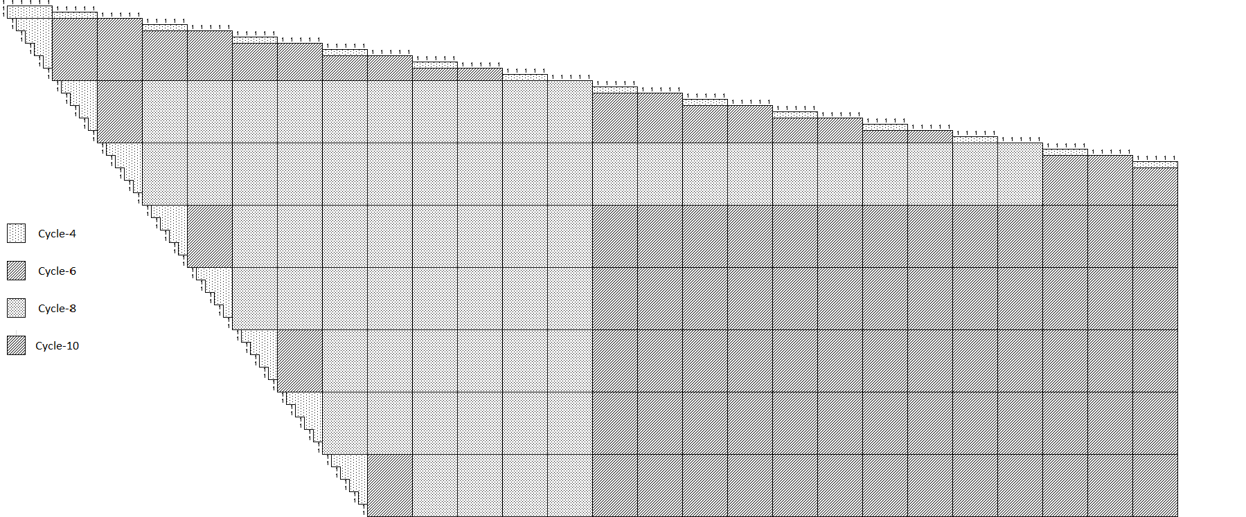
Figure 14: Subblocks and cycle regions with $J=3$ and $K=6$

In particular, when there is a 1 in a Cycle–4 region (dotted area), we have a cycle of length 4 as in the case of cycles $C_{1}$ and $C_{2}$ in Figure 15. We note that, Cycle–4 regions repeat both horizontally and vertically.

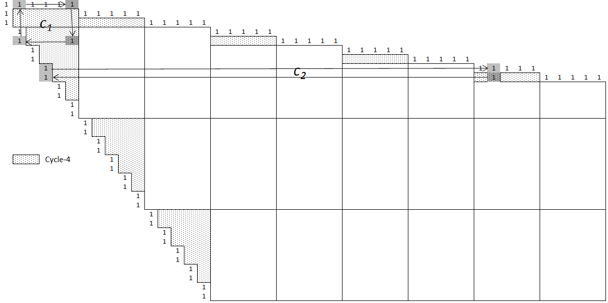
Figure 15: Cycle–4 regions with $J=3$ and $K=6$

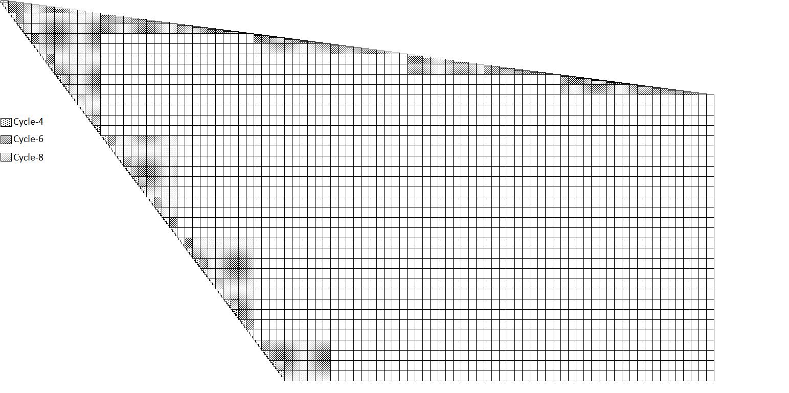
Figure 16: Cycle–4, Cycle–6, and Cycle–8 regions with $J=3$ and $K=6$

Similar horizontal and vertical repeating patterns can be seen for Cycle–6 and Cycle–8 regions in Figure 16. Making use of these patterns, one can express $\rho(i,j)$ of an entry $(i,j)$ as a function. We introduce valid inequalities for MDD based on the cycle region information of the entries in the reduced rectangle $R$.

Proposition 5.

Let $(i,j)\in R$, i.e., $i\in\{m-r_{cr},...,m\}$ and $j\in\{n-c_{cr},...,n\}$ and let $\rho(i,j)$ represent the cycle region of the entry. Let $S$ denote the number of subblocks that intersects with $R$ and let $B_{s}$, $s\in\{1,...,S\}$ represent the set of $(i,j)$ entries in subblock $s$.

1. If $\rho(i,j)<T$, then constraint

   $$X_{ij}=0$$ (14)

   is valid.

2. If $T=8$ and $(i,j)\in B_{s}$ with $\rho(i,j)=$ 8 or 10, then constraints

   $$\sum_{i=1}^{J-1}\sum_{((k-1)(J-1)+i,j)\in B_{s}}X_{(k-1)(J-1)+i,j}\leq 1,\ \ \ k\in\{1,...,K-1\}$$ (15)

   are valid.

3. If $T=10$ and $(i,j)\in B_{s}$ with $\rho(i,j)=10$, then constraint

   $$\sum_{(i,j)\in B_{s}}X_{ij}\leq 1$$ (16)

   is valid.

Proof. Let us consider each claim separately.

1. There cannot be cycles of length smaller than the girth $T$. If $X_{ij}=1$, then we have a cycle of length $\rho(i,j)<T$, which is not desired. Hence, $X_{ij}=0$ in this case.

2. If $T=8$, then there should not be any cycles of length 6. Let us consider a subblock with cycle region 8 or 10, which is subdivided into $(K-1)$ equal $subpieces$ each includes $(J-1)$ rows. In Figure 17, we give an example for Cycle–8 subblock with $J=3$ and $K=6$ where we have $(K-1)=5$ subpieces each having $(J-1)=2$ rows. As seen in figure, a cycle of length 6 forms when there is more than one nonzero entry in a subpiece.

   

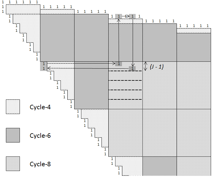
   Figure 17: A cycle of length 6 on Cycle–8 region with $J=3$ and $K=6$

   A similar case appears for Cycle–10 subblocks. Hence, constraints (15) are valid, since they force to have at most one nonzero entry in each subpiece when cycle region of the subblock is either 8 or 10.

   

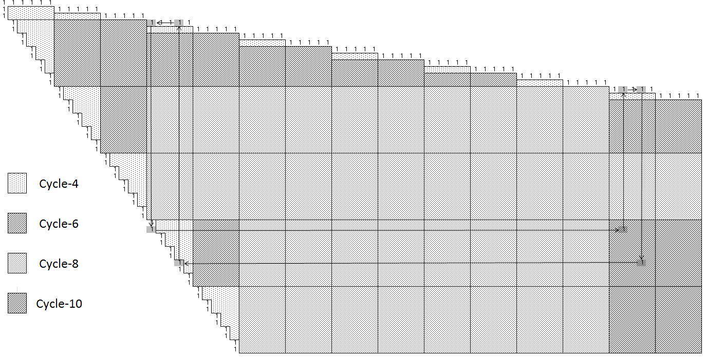
   Figure 18: A cycle of length 8 on Cycle–10 region with $J=3$ and $K=6$

3. A cycle of length 8 is not allowed when $T=10$. However, when there is more than one nonzero entry in a subblock with cycle region 10, there is a cycle of length 8 as given in Figure 18. Constraint (16) is valid, since it bounds the number of nonzero entries from above with 1. $\square$
   

Proposition 6.

Let $z^{*}$ be the optimum objective value of MDD and $z_{f}^{*}$ be the optimum objective value of MDD when variables are fixed with the $extended$ mode. Let $\tau$ be defined as in Proposition 2. Assume there exists a $(J,K)$–regular code with dimensions $(m,n)$, then

1. $0=z^{*}=z_{f}^{*}$ if $T>\tau$,

2. $0=z^{*}\leq z_{f}^{*}$ if $T\leq\tau$.

Proof. For any dimensions $(m,n)$, we have $z^{*}\leq z_{f}^{*}$, since we fix some $X_{ij}$ variables in the $extended$ mode. If there exists a $(J,K)$–regular code, then there is an optimal solution with objective value $z^{*}=0$. We know from Proposition 2 when $T>\tau$, a $(J,K)$–regular code can be expressed as in Figure 10, which coincides with the case in the $extended$ mode. Hence, we have $z_{f}^{*}=z^{*}=0$.

In MDD if $\rho(i,j)\geq T$, then $X_{ij}$ can be nonzero without harming the girth $T$. When $T\leq\tau$, there are $(i,j)\in S$ in Figure 10 with $\rho(i,j)\geq T$ and they are fixed to zero, since we fix all entries in the region $S$ to zero in the $extended$ mode. Then, we have $0=z^{*}\leq z_{f}^{*}$ in this case. $\square$

3.3.4 Modified Progressive Edge Growth Algorithm

The last improvement to our BC algorithm is to introduce a starting solution for an initial upper bound. For this purpose, we adapt an existing algorithm from the literature known as Progressive Edge Growth (PEG) algorithm [44]. We modify this algorithm for our problem by starting PEG from a partial initial solution generated by our fixing algorithm given in Algorithm 4. We also update PEG such that the generated solution has girth at least $T$. Time complexity of Algorithm 6 is the same with the original PEG, which is $\mathcal{O}(|V||E|+|E|^{2})$. In Algorithm 1, we set an upper bound by applying Algorithm 6 at step $(I.3)$.

Algorithm 6: (Modified PEG) Input: $(m,n)$ dimensions, $\mathbf{dv}$ and $\mathbf{dc}$ vectors, $T$ value 0. Initialize $\mathbf{X}\leftarrow\mathbf{0}$, $\mathbf{dv^{c}}\leftarrow\mathbf{0}$, $\mathbf{dv^{s}}\leftarrow\mathbf{dv}$ and $\mathbf{dc^{s}\leftarrow\mathbf{dc}}$, $\mathcal{I}\leftarrow\mathbf{0}$ 1. Apply Algorithm 4 and update slacks        $dv_{j}^{s}\leftarrow dv_{j}^{s}-\sum_{i}X_{ij}$ for all $j$ and $dc_{i}^{s}\leftarrow dc_{i}^{s}-\sum_{j}X_{ij}$ for all $i$        and current degrees $dv_{j}^{c}\leftarrow\sum_{i}X_{ij}$ for all $j$ 2. For $j\in\{1,...,n\}$ set $\mathcal{I}\leftarrow\mathbf{0}$ 3.      For $k\in\{0,...,dv_{j}^{c}\}$ 4.          If $k=0$, Then set $X_{i^{\prime}j}=1$ for $i^{\prime}=\operatornamewithlimits{argmax}_{i}\{dc_{i}^{s}\}$ 5.          Else apply BFS from $v_{j}$ to reach check nodes, let tree has depth $l$ 6.                 If $2l\geq T$ or $|\mathcal{N}_{j}^{l}|\leq m$, let $\mathcal{I}$ is incidence vector for $\mathcal{N}_{j}^{l}$                               set $X_{i^{\prime}j}=1$ for $i^{\prime}=\operatornamewithlimits{argmax}_{i}\{(1-\mathcal{I}_{c_{i}})dc_{i}^{s}\}$ 7.          End If 8.          Update $dv_{j}^{c}$, $dv_{j}^{s}$, $dc_{i}^{s}$ as in Step 1 9.      End For 10. End For Output: An initial solution for MDD

In Algorithm 6, $\mathbf{dv}$ and $\mathbf{dc}$ are the target degree vectors for variable and check nodes, respectively. Let deviation from the target degrees for variable and check nodes be given by slack vectors $\mathbf{dv^{s}}$ and $\mathbf{dc^{s}}$, and the current degrees of variable nodes be listed in vector $\mathbf{dv^{c}}$. Moreover, $\mathcal{N}_{j}^{l}$ represents the set of all check nodes that can be reached from $v_{j}$ with a tree of depth $l$. Hence, the set $\mathcal{N}_{j}^{l}\setminus\mathcal{N}_{j}^{l-1}$ collects the check nodes that are reached at the $l$th step from $v_{j}$ for the first time. We can represent the check nodes in the set $\mathcal{N}_{j}^{l}$ with an incidence vector $\mathcal{I}$ as $\mathcal{I}_{c_{i}}=1$ if $c_{i}\in\mathcal{N}_{j}^{l}$ and zero otherwise.

Starting from the solution provided by Algorithm 4, PEG adds an edge $(i,j)$, i.e., $X_{ij}=1$, if this edge does not form a cycle ($|\mathcal{N}_{j}^{l}|\leq m$) or the length of the cycle created is greater or equal to $T$ (Step 6). For edge assignment, the algorithm picks $c_{i}$ having the maximum slack value $dc_{i}^{s}$ in order to fit the target degree $dc_{i}$. The generated solution is feasible for MDD, since it has girth at least $T$.

4 Computational Results

The computations have been carried out on a computer with 2.0 GHz Intel Xeon E5–2620 processor and 46 GB of RAM working under Windows Server 2012 R2 operating system. In the computational experiments, we use CPLEX 12.6.2 to test the performance of BC algorithm and evaluate how different improvement strategies to BC algorithm given in Section 3.3 affect the results. We implement all algorithms in the C++ programming language. We summarize the solution methods in Table 2.

Table 2: Summary of solution methods

Method	Mode	Valid Inequalities	Modified PEG
BC0	–	–	–
BC1	$basic$	–	–
BC2	$extended$	–	–
BC3	$extended$	$\surd$	–
BC4	$extended$	$\surd$	$\surd$

In BC₀, we apply the BC algorithm in Algorithm 1 without improvement techniques, i.e., we exclude steps $(I.1)-(I.3)$. Algorithm 1 includes Algorithm 2 and 3 to separate integral and fractional solutions, respectively. In CPLEX, we implement Algorithm 2 using $LazyConstraintCallback$ and Algorithm 3 with $UserConstraintCallback$ routines. We utilize default branching settings of CPLEX. In BC₁ method, we apply step $(I.1)$ to fix the first row and column of $\mathbf{H}$ matrix in the $basic$ mode. In BC₂ method, step $(I.1)$ fixes $r_{cr}$ rows and $c_{cr}$ columns in the $extended$ mode (see Section 3.3.2). In BC₃ method, we apply step $(I.1)$ in the $extended$ mode and step $(I.2)$ adds valid inequalities that are explained in Section 3.3.3. Finally in BC₄ method, step $(I.1)$ runs in the $extended$ mode, step $(I.2)$ adds valid inequalities and step $(I.3)$ provides an initial solution with modified PEG (Algorithm 6).

We list the parameters used in the computational experiments in Table 3. We generate $(3,6)-$regular $\mathbf{H}$ matrices with girth values $T=6,8$ or 10 in our experiments. We try nine different $(m,n)$ dimensions from $n=20$ to 1000. We report the results that CPLEX found in 3600 seconds time limit.

Table 3: List of computational parameters

Parameters
$(J,K)$	$(3,6)-$regular codes
$(m,n)$	(10, 20), (15, 30), (20, 40), (30, 60),
	(40, 80), (100, 200), (150, 300), (250, 500), (500, 1000)
$T$	6, 8, 10
Time Limit	3600 secs

From Table 4 to 6, column “$z$” is the objective function value of MDD and column “$z_{l}$” is the best known lower bound found by CPLEX within the time limit. For each of the methods, we have an initial feasible solution (an upper bound) with objective value $z^{i}_{u}$. In BC₀ method, $\mathbf{H}=\mathbf{0}$ is a trivial solution providing an initial upper bound. In methods from BC₁ to BC₄ an initial feasible solution is obtained from variable fixing (see Section 3.3.2) or modified PEG heuristic (see Section 3.3.4). Computational time in seconds is given with column “CPU (secs)” and percentage difference among $z_{l}$ and $z$ is under column “Gap (%)”. In column “Lazy” we show number of cuts added to MDD using Algorithm 2, whereas column “User” is the number of cuts added to MDD with Algorithm 3.

As discussed in Section 3.1, we have a $(J,K)$–regular code if $z_{l}=z=0$. We can conclude that it is not possible to have a $(J,K)$–regular code with given $(m,n)$ and the girth $T$ when we have $z\geq z_{l}>0$ (see Proposition 3). In Table 4, we can see that BC₀ can find a $(3,6)-$regular code for 8 instances when $T=6$. As $T$ and $n$ increase, BC₀ method cannot improve initial upper bound $z^{i}_{u}$. For $T=8$ and $T=10$, we observe that the number of lazy and user cuts added to MDD gets smaller as $n$ gets larger. This is because adding a cut takes more time as $n$ increases, which causes the algorithm to generate fewer cuts within the given time limit.

Table 4: Computational results for BC₀

					CPU	Gap	# Cuts
$T$	$n$	$z_{l}$	$z$	$z^{i}_{u}$	(secs)	(%)	Lazy	User
6	20	0	20	120	$time$	100	7399	0
	30	0	0	180	13.80	0	5784	0
	40	0	0	240	0.39	0	331	0
	60	0	0	360	0.45	0	184	0
	80	0	0	480	0.41	0	94	0
	200	0	0	1200	1.06	0	238	0
	300	0	0	1800	2.62	0	165	0
	500	0	0	3000	4.72	0	114	0
	1000	0	0	6000	32.71	0	111	0
8	20	0	62	120	$time$	100	51759	19192
	30	0	86	180	$time$	100	138018	9890
	40	0	240	240	$time$	100	196066	4452
	60	0	360	360	$time$	100	285614	2683
	80	0	480	480	$time$	100	328598	2055
	200	0	1200	1200	$time$	100	404838	736
	300	0	1800	1800	$time$	100	327245	261
	500	0	3000	3000	$time$	100	207064	61
	1000	0	0	6000	905.21	0	2458	2
10	20	0	62	120	$time$	100	171969	31649
	30	0	164	180	$time$	100	393619	7676
	40	0	240	240	$time$	100	410765	5554
	60	0	360	360	$time$	100	554898	3740
	80	0	480	480	$time$	100	496226	2465
	200	0	1200	1200	$time$	100	67718	406
	300	0	1800	1800	$time$	100	22282	88
	500	0	3000	3000	$time$	100	11548	10
	1000	0	6000	6000	$time$	100	87546	65

Table 5 shows our computational results for BC₁ and BC₂. We have better initial upper bound ($z^{i}_{u}$) values compared to BC₀ when we implement variable fixing with the $basic$ mode in BC₁. We improve $z^{i}_{u}$ values more in BC₂ with the $extended$ mode, since we fix more entries compared to the $basic$ mode. We observe that $z_{l}=1$ for $T=6$ and $n=20$ in BC₁, which means it is not possible to have a $(3,6)-$regular code for this dimension. BC₁ method is able to solve 9 instances out of 27 instances to optimality, i.e., Gap (%) value is zero.

Table 5: Computational results for BC₁ and BC₂

		BC1								BC2
					CPU	Gap	# Cuts						CPU	Gap	# Cuts
$T$	$n$	$z_{l}$	$z$	$z^{i}_{u}$	(secs)	(%)	Lazy	User		$z_{l}$	$z$	$z^{i}_{u}$	(secs)	(%)	Lazy	User
6	20	1	20	104	$time$	95	3804	0		12	20	62	$time$	40	246	0
	30	0	0	164	23.11	0	7016	0		0	0	92	0.10	0	2532	0
	40	0	0	224	0.39	0	420	0		0	0	122	0.12	0	160	0
	60	0	0	344	0.37	0	124	0		0	0	182	0.20	0	148	0
	80	0	0	464	0.56	0	125	0		0	0	242	0.23	0	146	0
	200	0	0	1184	1.43	0	108	0		0	0	602	0.48	0	109	0
	300	0	0	1784	2.31	0	87	0		0	0	902	1.11	0	167	0
	500	0	0	2984	4.73	0	94	0		0	0	1502	2.44	0	225	0
	1000	0	0	5984	49.23	0	110	0		0	0	3002	21.83	0	165	0
8	20	0	44	104	$time$	100	19099	16644		42	42	62	0.08	0	0	0
	30	0	74	164	$time$	100	73701	8222		64	64	92	0.33	0	244	0
	40	0	92	224	$time$	100	131947	4385		56	84	122	$time$	32	2660	68
	60	0	344	344	$time$	100	225388	1903		12	80	182	$time$	85	25418	0
	80	0	464	464	$time$	100	240048	1703		0	242	242	$time$	100	61703	0
	200	0	1184	1184	$time$	100	407426	895		0	602	602	$time$	100	229615	0
	300	0	1784	1784	$time$	100	331382	487		0	902	902	$time$	100	292952	0
	500	0	2984	2984	$time$	100	216118	124		0	0	1502	1633.83	0	148866	0
	1000	0	0	5984	454.20	0	1386	6		0	0	3002	449.31	0	1263	0
10	20	0	58	104	$time$	100	57480	80057		54	54	62	0.09	0	0	0
	30	0	164	164	$time$	100	242023	16891		92	92	92	0.09	0	0	0
	40	0	224	224	$time$	100	342790	8174		122	122	122	0.11	0	0	0
	60	0	344	344	$time$	100	290718	3953		182	182	182	0.14	0	0	0
	80	0	464	464	$time$	100	471767	5285		236	236	242	142.56	0	3850	42
	200	0	1184	1184	$time$	100	51505	675		66	602	602	$time$	89	310451	1
	300	0	1784	1784	$time$	100	20565	135		0	902	902	$time$	100	461039	0
	500	0	2984	2984	$time$	100	9568	60		0	1502	1502	$time$	100	467420	0
	1000	0	5984	5984	$time$	100	90273	91		0	3002	3002	$time$	100	110798	0

In Table 5, we observe that we can solve 17 instances to optimality with BC₂ method. BC₂ finds $z_{l}>0$ for 11 instances indicating that there are no $(3,6)-$regular codes for those dimensions. There are 7 instances such as $T=10$ and $n=80$ that we have $z_{l}=z>0$. This means that for $n=80$ dimension, the best possible code with the girth $T=10$ includes $z/2=236/2=118$ fewer ones than a $(3,6)-$regular code (having $X_{ij}=1$ improves MDD objective by 2).

Comparing Table 5 and 6, we can see that $z^{i}_{u}$ values for BC₂ and BC₃ are the same, since we apply the $extended$ mode for both. On the other hand, feasible solution of Algorithm 6 (see Section 3.3.4) provides better $z^{i}_{u}$ values in BC₄. Results show that $z$ values get better, the number of cuts added to MDD gets smaller and computational time improves on the average as we have tighter initial solutions.

Table 6: Computational results for BC₃ and BC₄

		BC3								BC4
					CPU	Gap	# Cuts						CPU	Gap	# Cuts
$T$	$n$	$z_{l}$	$z$	$z^{i}_{u}$	(secs)	(%)	Lazy	User		$z_{l}$	$z$	$z^{i}_{u}$	(secs)	(%)	Lazy	User
6	20	12	20	62	$time$	40	260	0		13.9	20	26	$time$	37	238	0
	30	0	0	92	0.15	0	1784	0		0	0	8	0.22	0	2522	0
	40	0	0	122	0.14	0	160	0		0	0	2	0.36	0	441	0
	60	0	0	182	0.20	0	160	0		0	0	2	0.16	0	154	0
	80	0	0	242	0.24	0	148	0		0	0	2	0.33	0	184	0
	200	0	0	602	0.55	0	109	0		0	0	4	0.56	0	104	0
	300	0	0	902	1.02	0	167	0		0	0	2	1.11	0	167	0
	500	0	0	1502	3.33	0	225	0		0	0	2	3.05	0	207	0
	1000	0	0	3002	39.79	0	170	0		0	0	4	29.84	0	174	0
8	20	42	42	62	0.12	0	0	0		42	42	62	0.13	0	0	0
	30	64	64	92	0.16	0	0	0		64	64	86	0.13	0	0	0
	40	84	84	122	7.89	0	473	0		84	84	86	2.59	0	367	0
	60	28	64	182	$time$	56	55860	0		28	60	66	$time$	53	58432	0
	80	8	242	242	$time$	97	95449	0		8	38	38	$time$	87	83615	0
	200	0	0	602	2181.18	0	154415	0		0	0	16	1893.82	0	166949	0
	300	0	902	902	$time$	100	280596	0		0	10	10	$time$	100	284583	0
	500	0	0	1502	614.80	0	33635	0		0	0	10	1414.95	0	71447	0
	1000	0	0	3002	324.91	0	587	0		0	0	12	384.75	0	866	0
10	20	54	54	62	0.10	0	0	0		54	54	62	0.13	0	0	0
	30	92	92	92	0.09	0	0	0		92	92	92	0.11	0	0	0
	40	122	122	122	0.11	0	0	0		122	122	122	0.17	0	0	0
	60	182	182	182	0.11	0	0	0		182	182	182	0.13	0	0	0
	80	236	236	242	0.18	0	1	0		236	236	236	0.17	0	0	0
	200	260	602	602	$time$	57	100732	4		260	314	314	$time$	17	78306	16
	300	104	902	902	$time$	88	273318	0		104	274	274	$time$	62	335686	0
	500	0	1502	1502	$time$	100	170322	0		0	174	174	$time$	100	165584	0
	1000	0	3002	3002	$time$	100	52500	0		0	60	60	$time$	100	47637	0

In Table 6, we can also compare the performance of our methods with the state–of–the–art heuristic PEG. In BC₄ method, $z^{i}_{u}$ values are the objective function values of PEG. BC₄ method can improve the solution provided by PEG for 17 instances among 27 instances. Similarly, BC₁ outperfoms the PEG for 13 instances, BC₂ for 15 instances and BC₃ for 17 instances.

Table 7: Lower and upper bounds on the dimension $n$

	Proposition 3			BC4
$T$	$r_{cr}$	$n_{LB}$		$n_{LB}$	$n_{UB}$
6	3	20		20	30
8	13	70		80	200
10	33	170		300	—

Among the methods from BC₀ to BC₄, we can see that BC₄ uses the smallest number of cuts on the average and solves more instances to optimality (19 instances out of 27 instances). Besides, BC₄ provides an evidence that there cannot be a $(J,K)$–regular code (when $z_{l}>0$) for 13 instances within the given time limit. In Table 7, we compare the lower bounds on $n$ provided by Proposition 3 and BC₄ for a (3,6)–regular code with girth $T$. In BC₄ method, the largest $n$ that we have $z_{l}>0$ is a lower bound and the smallest $n$ that we obtain $z_{l}=z=0$ is an upper bound. BC₄ gives tighter lower bounds than Proposition 3. BC₄ can find the smallest dimension $n$ that one can generate a (3,6)–regular code with girth $T$ by applying binary search on $n$. Taking into account that code design problem is an offline problem, one can implement BC₄ method to construct a $(J,K)$–regular code providing sufficiently large time.

5 Conclusions

In this work, we investigate the LDPC code design problem and provide an MIP formulation for the girth feasibility problem. For the solution of the problem, we propose a branch–and–cut (BC) algorithm. We analyze structural properties of the problem and improve our BC algorithm by using techniques such as variable fixing, adding valid inequalities and providing an initial solution using a heuristic. Computational experiments indicate that each of these techniques improves BC one step further. Among all, the method that combines all of these strategies, i.e., BC₄ method, can solve the largest number of instances to optimality and gives the smallest gap values on average in an acceptable amount of time. One important gain of the method is that it can provide an evidence whether there can be a $(J,K)$–regular code with the given dimensions or not.

In this study, our focus has been on $(J,K)$–regular codes. In telecommunication applications, irregular LDPC codes are also utilized. Hence, extending these techniques to irregular LDPC codes can be a direction of future research. Spatially–coupled (SC) LDPC codes are another code family which has become popular due to their channel capacity approaching error correction capability. Design of SC LDPC codes without small cycles will be a valuable contribution to future communication standards.

References

- [1] J. D., Vacchione, R. C., Kruid, A., Prata, L. R., Amaro, and A. P., Mittskus, “Telecommunications antennas for the Juno mission to Jupiter,” Proc. IEEE Aerospace Conf., pp. 1–16, 2012.
- [2] R. G., Gallager, “Low–density parity–check codes,” IRE Trans. on Inf. Theory, vol 8, no. 1, pp. 21–28, January 1962.
- [3] R. M., Tanner, “A recursive approach to low complexity codes,” IEEE Trans. on Inf. Theory, vol IT-27, no. 5, pp. 533–547, September 1981.
- [4] J., Zhang, and M. P. C., Fossorier, “Shuffled iterative decoding,” IEEE Trans. on Commun., vol 53, no. 2, pp. 209–213, 2005.
- [5] J., Chen, A., Dholakia, E., Eleftheriou, M. P. C., Fossorier, and X. Y., Hu, “Reduced–complexity decoding of LDPC codes,” IEEE Trans. on Commun., vol 53, no. 8, pp. 1288–1299, 2005.
- [6] J. A., McGowan, and R. C., Williamson, “Loop removal from LDPC codes,” IEEE Inf. Theory Workshop, pp. 1–4, 2003.
- [7] S., Bandi, V., Tralli, A., Conti, and M., Nonato, “On girth conditioning for low–density parity–check codes,” IEEE Trans. on Commun., vol 59, no. 2, 2011.
- [8] I., Sason, “Linear programming bounds on the degree distributions of LDPC code ensembles,” Proc. IEEE Int. Symp. on Inf. Theory, pp. 224–228, 2009.
- [9] D., Pflüger, G., Bauch, “Optimization of variable edge degree distributions to compensate the differential penalty by LDPC turbo decoding,” Int. ITG Conf. on Systems, Commun. and Coding, pp. 1–6, 2015.
- [10] J., Compello, and D. S., Modha, “Extended bit–filling and LDPC code design,” Proc. IEEE Globecom Conf., vol 2, pp. 985–989, 25–29 November 2001.
- [11] L., Dinoi, F., Scottile, and S., Benedetto, “Design of variable–rate irregular LDPC codes with low error floor,” Proc. IEEE Int. Conf. on Commun., vol 1, pp. 647–651, 16–20 May 2005.
- [12] X. Y., Hu, E., Eleftheriou, and D. M., Arnold, “Regular and irregular progressive edge-growth Tanner graphs,” IEEE Trans. on Inf. Theory, vol 51, pp. 386–398, 2005.
- [13] H., Chen, and Z., Cao, “A modified PEG algorithm for construction of LDPC codes with strictly concentrated check–node degree distributions,” Proc. IEEE Wireless Commun. and Networking Conf., pp. 564–568, 11–15 March 2007.
- [14] C. T., Healy, and R. C., de Lamare, “Decoder–optimised progressive edge growth algorithms for the design of LDPC codes with low error floors,” IEEE Commun. Lett., vol 16, no. 6, pp. 889–892, June 2012.
- [15] E., Psota, and L. C., Pérez, “Iterative construction of regular LDPC codes from independent tree–based minimum distance bounds,” IEEE Commun. Lett., vol 15, no. 3, pp. 334–336, March 2011.
- [16] D., Divsalar, S., Dolinar, and C., Jones, “Low–rate LDPC codes with simple protograph structure,” Proc. IEEE Int. Symp. on Inf. Theory, pp. 1622–1626, 4–9 September 2005.
- [17] M., El-Khamy, J., Hou, and N., Bhushan, “Design of rate–compatible structured LDPC codes for hybrid ARQ applications,” IEEE J. on Selected Areas in Commun., vol 27, no. 6, pp. 965–973, August 2009.
- [18] A. K., Pradhan, A., Subramanian, and A., Thangaraj, “Deterministic constructions for large girth protograph LDPC codes,” Proc. IEEE Int. Symp. on Inf. Theory, pp. 1680–1684, 2013.
- [19] J., Lu, and J. M. F., Moura, “TS–LDPC codes: Turbo–structured codes with large girth,” IEEE Trans. on Inf. Theory, vol 53, no. 3, pp. 1080–1094, March 2007.
- [20] N., Bonello, S., Chen, and L., Hanzo, “Construction of regular quasi–cyclic protograph LDPC codes based on Vandermonde matrices,” IEEE Trans. on Vehicular Technology, vol 57, no. 4, pp. 2583–2588, July 2008.
- [21] H., Zhao, X., Bao, L., Qin, R., Wang, and H., Zhang, “Construction of irregular QC–LDPC codes in near–earth communications,” Journal of Communications, vol 9, no. 7, pp. 541–547, 2014.
- [22] Z., Li, and B. V. K. V., Kumar, “A class of good quasi–cyclic low–density parity check codes based on progressive edge growth graph,” Conf. Record of the Thirty–Eight Asilomar Conf. on Signals, Systems and Computers, vol 2, pp. 1990–1994, 7–10 November 2004.
- [23] P., Prompakdee, W., Phakphisut, and P., Supnithi, “Quasi cyclic–LDPC codes based on PEG algorithm with maximized girth property,” Proc. Int. Symp. on Intelligent Signal Processing and Commun. Syst. (ISPACS), pp. 1–4, December 2011.
- [24] L., Kong, L., He, P., Chen, G., Han, and Y., Fang, “Protograph–based quasi–cyclic LDPC coding for ultrahigh density magnetic recording channels,” IEEE Trans. on Magnetics, vol 51, no. 11, 2015.
- [25] X., Jiang, M. H., Lee, H., Wang, J., Li, and M., Wen, “Modified PEG algorithm for large girth quasi–cyclic protograph LDPC codes,” Proc. Int. Conf. on Computing, Networking and Communications, Mobile Computing and Vehicle Communications, 2016.
- [26] S., Myung, K., Yang, and J., Kim, “Lifting methods for quasi–cyclic LDPC codes,” IEEE Commun. Lett., vol 10, no. 6, pp. 489–491, June 2006.
- [27] Z., Liu, and D. A., Pados, “LDPC codes from generalized polygons,” IEEE Trans. on Inf. Theory, vol 51, no. 11, pp. 3890–3898, November 2005.
- [28] J., Yedidia, and Y., Wang, “Method for determining quasi–cyclic low–density parity–check code, and system for encoding data based on quasi–cyclic low–density parity–check code,” WO Patent 2013047258 A1, 4 April 2013.
- [29] I. E., Bocharova, B. D., Kudryashov, and R., Johannesson, “Combinatorial optimization for improving QC LDPC codes performance,” Proc. IEEE Int. Symp. on Inf. Theory, pp. 2651–2655, 2013.
- [30] X., He, L., Zhou, J., Du, and Z., Shi, “The multi–step PEG and ACE constrained PEG algorithms can design the LDPC codes with better cycle–connectivity,” Proc. IEEE Int. Symp. on Inf. Theory, pp. 46–50, 2015.
- [31] A., Beemer, and C. A., Kelley, “Avoiding trapping sets in SC–LDPC codes under windowed decoding,” Proc. IEEE Int. Symp. on Inf. Theory and Its Applicat., pp. 206–210, 2016.
- [32] I. E., Bocharova, R. Johannesson, and B. D., Kudryashov, “A unified approach to optimization of LDPC codes for various communication scenarios,” Proc. IEEE Int. Symp. on Turbo Codes and Iterative Inf. Processing, pp. 243–248, 2014.
- [33] X., Jiang, H., Hai, H., Wang, and M. H., Lee, “Constructing large girth QC protograph LDPC codes based on PSD–PEG algorithm,” IEEE Access, 2017.
- [34] J., Broulim, S., Davarzani, V., Georgiev, and J., Zich, “Genetic optimization of a short block length LDPC code accelerated by distributed algorithms,” Proc. IEEE Telecommun. Forum, pp. 1–4, 2016.
- [35] S., Shebl, M., Shokair, and A., Gomaa, “Novel construction and optimization of LDPC codes for NC-OFDM cognitive radio systems,” Wireless Personal Communications, pp. 69–83, 2014.
- [36] B. M. J., Leiner, “LDPC codes - a brief tutorial,” Wien Technical University, 2005.
- [37] A., Shokrollahi, “LDPC codes: an introduction,” Digital Fountain, Inc., 2003.
- [38] T., Richardson, “Error floors for LDPC codes,” Proc. Allerton Conferance on Commun. Control and Computing, vol 41, no. 3, pp. 1426–1435, September 2003.
- [39] R., Diestel, Graph Theory. 4th ed. Berlin, Germany: Springer–Verlag, June 2010.
- [40] R. K., Ahuja, T. L., Magnanti, and J. B., Orlin, Network Flows, Theory, Algorithms and Applications. 1st ed. New Jersey, USA: Prentice Hall, 1993.
- [41] R., Jans, and J., Desrosiers, “Efficient symmetry breaking formulations for the job grouping problem,” Computers and Operations Research, vol 40, pp. 1132–1142, 2013.
- [42] H. D., Sherali, and J. C., Smith, “Improving discrete model representations via symmetry considerations,” Management Science, vol 47, no. 10, pp. 1396–1407, 2001.
- [43] Y., Xiao, Y., Xie, S., Kulturel-Konak, and A., Konak, “A problem evolution algorithm with linear programming for the dynamic facility layout problem–A general layout formulation,” Computers and Operations Research, vol 88, pp. 187–207, 2017.
- [44] X. Y., Hu, E., Eleftheriou, and D. M., Arnold, “Progressive edge-growth Tanner graphs,” Proc. IEEE Global Telecommunications Conf., vol 2, pp. 995–1001, 2001.