Abstract

It is shown that neutrino oscillation processes can be consistently described in the framework of quantum field theory. Namely, the oscillating electron survival probabilities in experiments with neutrino detection by charged-current and neutral-current interactions are calculated in the quantum field-theoretical approach to neutrino oscillations based on a modification of the Feynman propagator. The approach is most similar to the standard Feynman diagram technique in the momentum representation. It is found that the oscillating distance-dependent probabilities of detecting an electron in experiments with neutrino detection by charged-current and neutral-current interactions exactly coincide with the corresponding probabilities calculated in the standard approach.

1 Introduction

Neutrino oscillation is a well-known and experimentally confirmed phenomenon, which is usually understood as the transition from a neutrino flavor state to another neutrino flavor state depending on the distance traveled [1, 2, 3]. However, the situation with the theoretical explanation of this phenomenon is paradoxical: the phenomenon, which is both quantum and relativistic, cannot be consistently described in the framework of quantum field theory, which is a synthesis of quantum mechanics and special theory of relativity. The standard theoretical description of this phenomenon based on the notion of neutrino flavor states is not perfect: the neutrino flavor states are superpositions of the neutrino mass eigenstates, and for this reason the processes with the flavor states cannot be consistently described within quantum field theory. The problem is the violation of energy-momentum conservation in such processes, because in local quantum field theory, where the four-momentum is conserved in any interaction vertex, different mass-eigenstate components of the flavor states must have different momenta as well as different energies. This problem was repeatedly discussed in the literature (see, e.g. [4, 5, 6, 7]).

A possible solution to the problem with the violation of energy-momentum conservation is to go off the mass shell. It was first discussed in paper [4], where it was suggested that the produced neutrino mass eigenstates are virtual and their motion to the detection point should be described by the Feynman propagators. Later this approach was developed in papers [5, 6]. However, the calculations in these papers imply the use of wave packets and are essentially different from the standard calculations in the framework of the Feynman diagram technique in the momentum representation. This is due to the standard S-matrix formalism of QFT used in these papers, which is not appropriate for describing processes at finite distances and finite time intervals.

In the present paper we will show that neutrino oscillation can be consistently described in the framework of quantum field theory. Namely, we will explicitly calculate the probabilities of the neutrino oscillation processes in experiments with neutrino detection by charged-current and neutral-current interactions within a modified perturbative S-matrix formalism, which enables one to calculate the amplitudes of the processes passing at finite distances and finite time intervals. This formalism was put forward in paper [8]. It is based on the Feynman diagram technique in the coordinate representation [9] supplemented by new modified rules of passing to the momentum representation, which will be discussed below in detail.

2 Oscillations in experiments with neutrino detection by charged-current interaction

In the framework of the minimal extension of the Standard Model (SM) by the right neutrino singlets we consider the case, where the neutrinos are produced and detected in the charged-current interaction with nuclei. After the diagonalization of the terms sesquilinear in the neutrino fields, the charged-current interaction Lagrangian of leptons takes the form

$$L_{cc}=-\frac{g}{2\sqrt{2}}\left(\sum_{i,k=1}^{3}\bar{l}_{i}\gamma^{\mu}(1-\gamma^{5})U_{ik}\nu_{k}W^{-}_{\mu}+h.c.\right),$$ (1)

where $l_{i}$ denotes the field of the charged lepton of the i-th generation, $\nu_{i}$ denotes the field of the neutrino mass eigenstate most strongly coupled to $l_{i}$ and $U_{ik}$ stands for the Pontecorvo-Maki-Nakagawa-Sakata (PMNS) matrix. Due to this structure of the interaction Lagrangian any process involving the production of a neutrino at one point and its detection at another point, when treated perturbatively, can be represented in the lowest order by the following diagram,

which should be summed over all three neutrino mass eigenstates. To be specific, we assume that the virtual $W$-bosons are produced and absorbed in interactions with nuclei. Namely, we suppose that a nucleus ${}^{A_{1}}_{Z_{1}}X$ that will be called nucleus $1$ radiates $W^{+}$-boson and turns into the nucleus ${}^{A_{1}}_{Z_{1}-1}X$ that will be called nucleus $1^{\prime}$, and a nucleus ${}^{A_{2}}_{Z_{2}}X$ that will be called nucleus $2$ absorbs $W^{+}$-boson and turns into the nucleus ${}^{A_{2}}_{Z_{2}+1}X$ that will be called nucleus $2^{\prime}$. Thus, the filled circles stand for the matrix elements of the charged weak hadron current

$$j_{\mu}^{(1)}=\left<{}^{A_{1}}_{Z_{1}-1}X\right|j_{\mu}^{(h)}\left|{}^{A_{1}}_{Z_{1}}X\right>,\quad j_{\rho}^{(2)}=\left<{}^{A_{2}}_{Z_{2}+1}X\right|j_{\rho}^{(h)}\left|{}^{A_{2}}_{Z_{2}}X\right>,$$

associated with nuclei $1,1^{\prime}$ and $2,2^{\prime}$. As it is customary in QFT, we assume that the incoming nuclei 1 and 2 have definite momenta. Therefore all the three virtual neutrino eigenstates and the outgoing particles and nuclei also have definite momenta. In what follows, a 4-momentum of the virtual neutrino mass eigenstates defined only by the energy-momentum conservation in the production vertex will be denoted by $p_{n}$ and the one selected also by the experimental setting will be denoted by $p$.

The amplitude in the coordinate representation corresponding to diagram (2) can be written out in the standard way using the Feynman rules formulated in textbook [10]. According to the prescriptions of the standard perturbative S-matrix theory ([10], §24), in order to obtain the amplitude in the momentum representation next we would have to integrate it with respect to $x$ and $y$ over the Minkowski space. However, in this case we would get the amplitude of the process lasting an infinite amount of time and lose the information about the distance between the production and detection points defined by the experimental setting. In order to retain this information, we have to integrate with respect to $x$ and $y$ in such a way that the distance between these points along the direction of the neutrino propagation remains fixed. Of course, this is at variance with the standard S-matrix formalism. However, we recall that the diagram technique in the coordinate representation was developed by R. Feynman [9] without reference to S-matrix theory. Thus, the Feynman diagrams in the coordinate representation make sense beyond this theory, and for this reason we can integrate with respect to $x$ and $y$ in any way depending on the physical problem at hand. In particular, in the case under consideration we have to integrate in such a way that the distance between the points $x$ and $y$ along the direction of the propagation of neutrino with momentum $\vec{p}$ defined by the experimental setting equals to $L$. This can be achieved by introducing the delta function $\delta(\vec{p}(\vec{y}-\vec{x})/|\vec{p}|-L)$ into the integral, which is equivalent to replacing the standard Feynman propagator of the neutrino mass eigenstate $\nu_{i}$ in the coordinate representation $S^{c}_{i}(y-x)$ by $S^{c}_{i}(y-x)\delta(\vec{p}(\vec{y}-\vec{x})/|\vec{p}|-L)$. The Fourier transform of the latter expression was called in paper [8] the distance-dependent propagator of the neutrino mass eigenstate $\nu_{i}$ in the momentum representation. It will be denoted by $S^{c}_{i}(p,L)$ and is defined by the integral:

$$S^{c}_{i}(p,L)=\int dx\,e^{ipx}S^{c}_{i}(x)\,\delta(\vec{p}\vec{x}/|\vec{p}|-L).$$ (3)

This integral can be evaluated exactly by the method of contour integration [8], and for $\vec{p}^{\,2}>m_{i}^{2}-p^{2}$ the result is given by

$$S^{c}_{i}(p,L)=i\,\frac{\hat{p}+\vec{\gamma}\vec{p}\left(1-\sqrt{1+\frac{p^{2}-m_{i}^{2}}{\vec{p}^{\,2}}}\,\right)+m_{i}}{2\sqrt{\vec{p}^{\,2}+p^{2}-m_{i}^{2}}}\,e^{-i\left(|\vec{p}|-\sqrt{\vec{p}^{\,2}+p^{2}-m_{i}^{2}}\,\right)L}\,.$$ (4)

(In paper [8] this distance-dependent propagator was defined by substituting the dimensionless delta function $\delta(\vec{p}\vec{x}-|\vec{p}|L)$ into the integral, which results in an extra factor $|\vec{p}|$ in the denominator of $S^{c}_{i}(p,L)$. Below we will see that the present definition is more natural.) We emphasize that this distance-dependent fermion propagator makes sense only for macroscopic distances $L$.

The results of paper [5] imply that the virtual particles propagating at macroscopic distances are almost on the mass shell. This means that $|p^{2}-m_{i}^{2}|/\vec{p}^{\,2}\ll 1$ and we can expand the square roots to the first order in $(p^{2}-m_{i}^{2})/\vec{p}^{\,2}$. It is clear that this term can be dropped everywhere, except in the exponential, where it is multiplied by a large macroscopic distance $L$. In this approximation distance-dependent propagator (4) takes the simple form

$$S^{c}_{i}(p,L)=i\,\frac{\hat{p}+m_{i}}{2|\vec{p}|}\,e^{-i\frac{m_{i}^{2}-p^{2}}{2|\vec{p}|}L}\,.$$ (5)

It is worth noting that this distance-dependent fermion propagator taken on the mass shell has no pole and does not depend on the distance, which is also true for the exact propagator in formula (4).

In fact, we have discussed this distance-dependent propagator in order to explain better the motivations for introducing such an object, because it exactly corresponds to the experimental situation in neutrino oscillation processes. However, this distance-dependent propagator is not convenient for calculating amplitudes, because there is no inverse Fourier transformation for the propagator in formula (3). It turns out that a more convenient and a more fundamental object is the time-dependent propagator of the neutrino mass eigenstates, which can be defined as the Fourier transform of $S^{c}_{i}(x)\delta(x^{0}-T)$. A similar time-dependent scalar field propagator was introduced in paper [8]. Using the results of the calculations of the time-dependent scalar field propagator in this paper one can easily find that the time-dependent fermion field propagator in the momentum representation is

$$S^{c}_{i}(p_{n},T)=i\,\frac{\hat{p}_{n}-\gamma^{0}\left(p_{n}^{\,0}-\sqrt{(p_{n}^{\,0})^{2}+m_{i}^{2}-p_{n}^{2}}\,\right)+m_{i}}{2\sqrt{(p_{n}^{\,0})^{2}+m_{i}^{2}-p_{n}^{2}}}\,e^{i\left(p_{n}^{\,0}-\sqrt{(p_{n}^{\,0})^{2}+m_{i}^{2}-p_{n}^{2}}\,\right)T}\,.$$ (6)

The advantage of the time-dependent propagator is that there exists the inverse Fourier transformation of this propagator, which allows one to retain the standard rules of the Feynman diagram technique just by replacing the Feynman propagator by this time-dependent propagator. For macroscopic time intervals $T$, i.e. for the particles close to the mass shell, it looks explicitly like

$$S^{c}_{i}(p_{n},T)=i\,\frac{\hat{p}_{n}+m_{i}}{2p_{n}^{\,0}}\,e^{-i\frac{m_{i}^{2}-p_{n}^{2}}{2p_{n}^{\,0}}T}\,.$$ (7)

In case all the neutrinos in a beam have the same momentum $p$ defined by the experimental setting we can express the time $T$ in terms of the distance $L$ and the neutrino speed $|\vec{p}|/p^{\,0}$ as $T=Lp^{\,0}/|\vec{p}|$, neglect the neutrino mass that is small compared to $\hat{p}$ and get a distance-dependent propagator

$$S^{c}_{i}(p,L)=i\,\frac{\hat{p}}{2p^{\,0}}\,e^{-i\frac{m_{i}^{2}-p^{2}}{2|\vec{p}|}L}\,,$$ (8)

which coincides with the above defined distance-dependent propagator of neutrinos (5) in the approximation of small neutrino masses. In what follows, we will use propagators (7), (8) for describing neutrino oscillation processes. We also note that the time-dependent scalar field propagator is adequate for calculating the probabilities of oscillation processes with massive scalar mesons, where we cannot neglect their masses.

Now we will calculate the amplitude corresponding to diagram (2) in the case, where the time difference $y^{0}-x^{0}$ is fixed and equal to $T$. Since the momentum transfer in both production and detection processes is small, we can use the approximation of Fermi’s interaction. Then making use of time-dependent propagator (7) and keeping the neutrino masses only in the exponential we can explicitly write out the amplitude in the momentum representation corresponding to diagram (2) summed over all three neutrino mass eigenstates:

$$M=-i\frac{{G_{F}^{\,2}}}{4{p_{n}^{\,0}}}\sum\limits_{i=1}^{3}{\left|{U_{1i}}\right|^{2}e^{-i\frac{m_{i}^{2}-p_{n}^{2}}{2p_{n}^{\,0}}T}}j_{\rho}^{(2)}\bar{u}\left(k\right)\gamma^{\rho}\left({1-\gamma^{5}}\right)\hat{p}_{n}\gamma^{\mu}\left({1-\gamma^{5}}\right)v\left(q\right)j_{\mu}^{(1)}.$$ (9)

Here $j_{\mu}^{(1)}$ and $j_{\rho}^{(2)}$ stand for the matrix elements of the charged weak hadron current associated with nuclei $1,1^{\prime}$ and $2,2^{\prime}$; $k$, $p_{n}$ and $q$ are the 4-momenta of the electron, the intermediate virtual neutrinos and the positron, respectively, and we do not write out explicitly the fermion polarization indices.

Averaging with respect to the polarizations of the incoming nuclei and summing over the polarizations of the outgoing particles and nuclei one gets the expression for the squared amplitude as follows:

$$\left\langle{\left|M\right|^{2}}\right\rangle=\frac{{4G_{F}^{\,4}}}{{\left(p^{\,0}_{n}\right)^{2}}}W_{\mu\nu}^{(1)}A^{\mu\nu\rho\sigma}W_{\rho\sigma}^{(2)}\left[{1-4\sum\limits_{\scriptstyle i,k=1\hfill\atop\scriptstyle i<k\hfill}^{3}{\left|{U_{1i}}\right|^{2}\left|{U_{1k}}\right|^{2}\sin^{2}\left({\frac{{m_{i}^{2}-m_{k}^{2}}}{{4{p^{\,0}_{n}}}}T}\right)}}\right],$$ (10)

where

$$A^{\mu\nu\rho\sigma}=\frac{1}{64}tr\left(\hat{p}_{n}\gamma^{\mu}\left({1-\gamma^{5}}\right)\left(\hat{q}-m\right)\gamma^{\nu}\left({1-\gamma^{5}}\right)\hat{p}_{n}\gamma^{\sigma}\left({1-\gamma^{5}}\right)\left(\hat{k}+m\right)\gamma^{\rho}\left({1-\gamma^{5}}\right)\right)$$

(the factor ${\raise 2.15277pt\hbox{$\scriptstyle 1$}\kern-1.00006pt/\kern-1.49994pt\lower 1.07639pt\hbox{$\scriptstyle{64}$}}$ is introduced in order to separate the numerical coefficient from the Lorentz structure proper), the tensors $W_{\mu\nu}^{(1)},\,W_{\rho\sigma}^{(2)}$ characterizing the interaction of nuclei $1$ and $2$ with virtual $W$-bosons are defined as

$$W_{\mu\nu}^{(1)}=\left\langle{j_{\mu}^{(1)}\left({j_{\nu}^{(1)}}\right)^{+}}\right\rangle,\qquad W_{\rho\sigma}^{(2)}=\left\langle{j_{\rho}^{(2)}\left({j_{\sigma}^{(2)}}\right)^{+}}\right\rangle.$$ (11)

Here and below the angle brackets denote the averaging with respect to the polarizations of the incoming particles and the summation over the polarizations of the outgoing particles, i.e. in the previous formula they denote the averaging with respect to the polarizations of nuclei $1,2$ and the summation over the polarizations of nuclei $1^{\prime},2^{\prime}$.

Since we have dropped the neutrino masses in the time-dependent propagators, we have actually calculated the amplitude in the approximation of zero neutrino masses. As we have already noted, for macroscopic time intervals $T$ the virtual neutrinos are almost on the mass shell and, therefore, the squared momentum of the virtual neutrinos $p_{n}^{2}$ is also of the order of the neutrino masses squared and can be neglected. In other words, we may calculate the squared amplitude in the approximation $p_{n}^{2}=0$. Direct calculations show that in this approximation the tensor $A^{\mu\nu\rho\sigma}$ factorizes:

$$A^{\mu\nu\rho\sigma}=\left(-g^{\mu\nu}({p_{n}q})+(p_{n}^{\mu}q^{\nu}+q^{\mu}p_{n}^{\nu})+i\varepsilon^{\mu\nu\alpha\beta}p_{n\alpha}q_{\beta}\right)\left(-g^{\rho\sigma}({p_{n}k})+(p_{n}^{\rho}k^{\sigma}+k^{\rho}p_{n}^{\sigma})-i\varepsilon^{\rho\sigma\alpha\beta}p_{n\alpha}k_{\beta}\right).$$ (12)

Correspondingly, the squared amplitude in formula (10) factorizes as follows:

$$\left\langle{\left|M\right|^{2}}\right\rangle = \left\langle{\left|M_{1}\right|^{2}}\right\rangle\left\langle{\left|M_{2}\right|^{2}}\right\rangle\frac{{1}}{{4\left({p^{\,0}_{n}}\right)^{2}}}\left[{1-4\sum\limits_{\scriptstyle i,k=1\hfill\atop\scriptstyle i<k\hfill}^{3}{\left|{U_{1i}}\right|^{2}\left|{U_{1k}}\right|^{2}\sin^{2}\left({\frac{{m_{i}^{2}-m_{k}^{2}}}{{4p^{\,0}_{n}}}T}\right)}}\right],$$ (13)

$$\left\langle{\left|M_{1}\right|^{2}}\right\rangle = 4G_{F}^{\,2}\left(-{g^{\mu\nu}\left({p_{n}q}\right)+\left({p_{n}^{\mu}q^{\nu}+q^{\mu}p_{n}^{\nu}}\right)+i\varepsilon^{\mu\nu\alpha\beta}p_{n\alpha}q_{\beta}}\right)W_{\mu\nu}^{(1)},$$ (14)

$$\left\langle{\left|M_{2}\right|^{2}}\right\rangle = 4G_{F}^{\,2}\left(-{g^{\rho\sigma}\left({p_{n}k}\right)+\left({p_{n}^{\rho}k^{\sigma}+k^{\rho}p_{n}^{\sigma}}\right)-i\varepsilon^{\rho\sigma\alpha\beta}p_{n\alpha}k_{\beta}}\right)W_{\rho\sigma}^{(2)}.$$ (15)

Here $\left\langle{\left|M_{1}\right|^{2}}\right\rangle$ is the squared amplitude of the decay process of nucleus $1$ into nucleus $1^{\prime}$, positron and a massless fermion and $\left\langle{\left|M_{2}\right|^{2}}\right\rangle$ is the squared amplitude of the process of electron production in the collision of the massless fermion and nucleus $2$.

Now we are in a position to calculate the probability of the process depicted in diagram (2), when the time difference between the points $x$ and $y$ is equal to $T$. We will do these calculations in accordance with the rules of the standard perturbative S-matrix theory, although we are aware that the rules of calculating the probabilities of processes passing at finite time interval and finite distances may be different from those of the standard S-matrix theory. We will discuss this difference below. To this end we denote the 4-momenta of the nuclei by $P^{(i)}=(E^{(i)},\vec{P}^{(i)}),\ P^{(i^{\prime})}=(E^{(i^{\prime})},\vec{P}^{(i^{\prime})}),\ i=1,2$, and recall that the amplitude in the momentum representation corresponding to diagram (2) contains, along with the expression in formula (9), the delta function of energy-momentum conservation. Thus, to calculate the probability of the process per unit time per unit volume, we have to multiply amplitude (13) by $(2\pi)^{4}\delta(P^{(1)}+P^{(2)}-P^{(1^{\prime})}-P^{(2^{\prime})}-q-k)$ and to integrate it with respect to the momenta of the outgoing particles and nuclei.

Since the momentum $p_{n}$ of the virtual neutrinos is defined by the energy-momentum conservation in the production vertex, $p_{n}=P^{(1)}-P^{(1^{\prime})}-q$, this integration can lead to variation in the virtual neutrino momentum, which contradicts the experimental situation in neutrino oscillations, where the virtual neutrinos propagate in the direction defined by the relative position of a source and a detector. This means that we have to calculate the differential probability of the process with $p_{n}$ fixed by the experimental setting.

Let us denote by $\vec{p}$ the momentum that is directed from the source to the detector and satisfies the momentum conservation condition $\vec{P}^{(1)}-\vec{P}^{(1^{\prime})}-\vec{q}-\vec{p}=0$ in the production vertex and define the four-momentum $p=(p^{\,0},\vec{p}),\,p^{\,0}>0,\,p^{2}=0$. The required differential probability of the process with $p_{n}$ fixed can be obtained by multiplying amplitude (13) by the delta function $\delta(p_{n}-p)$ or, equivalently, by replacing $p_{n}$ by $p$ in the amplitude and multiplying it by $\delta(P^{(1)}-P^{(1^{\prime})}-q-p)$. This is consistent, because we work in the approximation of massless neutrinos.

Thus, the differential probability takes the form:

$$\frac{dW}{dp} = \frac{{G_{F}^{4}}}{{16\left({2\pi}\right)^{8}E^{(1)}E^{(2)}\left({p^{\,0}}\right)^{2}}}\left[{1-4\sum\limits_{\scriptstyle i,k=1\hfill\atop\scriptstyle i<k\hfill}^{3}{\left|{U_{1i}}\right|^{2}\left|{U_{1k}}\right|^{2}\sin^{2}\left({\frac{{m_{i}^{2}-m_{k}^{2}}}{{4{p^{\,0}}}}T}\right)}}\right]\times$$ (16)

$$\times\int{d^{3}qd^{3}P^{(1^{\prime})}d^{3}kd^{3}P^{(2^{\prime})}\frac{1}{{q^{0}E^{(1^{\prime})}k^{0}E^{(2^{\prime})}}}}\times$$

$$\times\left({g^{\mu\nu}\left({pq}\right)-\left({p^{\mu}q^{\nu}+q^{\mu}p^{\nu}}\right)-i\varepsilon^{\mu\nu\alpha\beta}p_{\alpha}q_{\beta}}\right)W_{\mu\nu}^{(1)}\left({P^{(1)},P^{(1^{\prime})}}\right)\times$$

$$\times\left({g^{\rho\sigma}\left({pk}\right)-\left({p^{\rho}k^{\sigma}+k^{\rho}p^{\sigma}}\right)+i\varepsilon^{\rho\sigma\alpha\beta}p_{\alpha}k_{\beta}}\right)W_{\rho\sigma}^{(2)}\left({P^{(2)},P^{(2^{\prime})}}\right)\times$$

$$\times\delta\left({P^{(1)}+P^{(2)}-P^{(1^{\prime})}-P^{(2^{\prime})}-q-k}\right)\delta\left({P^{(1)}-P^{(1^{\prime})}-q-p}\right).$$

It is easy to verify that, due to the factorization of the squared amplitude, this differential probability also factorizes. Now, since the momentum of virtual neutrinos is fixed, we can replace $T$ by $Lp^{\,0}/|\vec{p}|$, as it was explained after formula (7), which gives

$$\frac{{dW}}{{dp}}=\frac{1}{{2\pi}}\frac{{dW_{1}}}{{d\vec{p}}}W_{2}\left[{1-4\sum\limits_{\scriptstyle i,k=1\hfill\atop\scriptstyle i<k\hfill}^{3}{\left|{U_{1i}}\right|^{2}\left|{U_{1k}}\right|^{2}\sin^{2}\left({\frac{{m_{i}^{2}-m_{k}^{2}}}{{4\left|{\vec{p}}\right|}}L}\right)}}\right],$$ (17)

where

$$\frac{{dW_{1}}}{{d\vec{p}}} = \frac{1}{{2E^{(1)}}}\frac{1}{{\left({2\pi}\right)^{3}}}\frac{1}{{2p^{\,0}}}\int{\frac{{d^{3}q}}{{\left({2\pi}\right)^{3}}}\frac{1}{{2q^{0}}}\frac{{d^{3}P^{(1^{\prime})}}}{{\left({2\pi}\right)^{3}}}\frac{1}{{2E^{(1^{\prime})}}}\left\langle{\left|{M_{1}}\right|^{2}}\right\rangle\left({2\pi}\right)^{4}\delta\left({P^{(1)}-P^{(1^{\prime})}-q-p}\right)}=$$ (18)

$$= \frac{{G_{F}^{2}}}{{4\left({2\pi}\right)^{5}E^{(1)}p^{\,0}}}\int{d^{3}qd^{3}P^{(1^{\prime})}\frac{1}{{q^{0}E^{(1^{\prime})}}}\left({-g^{\mu\nu}\left({pq}\right)+\left({p^{\mu}q^{\nu}+q^{\mu}p^{\nu}}\right)+i\varepsilon^{\mu\nu\alpha\beta}p_{\alpha}q_{\beta}}\right)\times}$$

$$\times W_{\mu\nu}^{(1)}\left({P^{(1)},P^{(1^{\prime})}}\right)\delta\left({P^{(1)}-P^{(1^{\prime})}-q-p}\right)$$

is the differential probability of the decay of nucleus $1$ into nucleus $1^{\prime}$, positron and a massless fermion with momentum $\vec{p}$, which coincides with the sum of the differential probabilities of the decay of nucleus $1$ into nucleus $1^{\prime}$, positron and all the three neutrino mass eigenstates, and

$$W_{2} = \frac{1}{{2E^{(2)}2p^{\,0}}}\int{\frac{{d^{3}k}}{{\left({2\pi}\right)^{3}}}\frac{1}{{2k^{0}}}\frac{{d^{3}P^{(2^{\prime})}}}{{\left({2\pi}\right)^{3}}}\frac{1}{{2E^{(2^{\prime})}}}\left\langle{\left|{M_{2}}\right|^{2}}\right\rangle\left({2\pi}\right)^{4}\delta\left({P^{(2)}+p-P^{(2^{\prime})}-k}\right)}=$$ (19)

$$= \frac{{G_{F}^{2}}}{{4\left({2\pi}\right)^{2}E^{(2)}p^{\,0}}}\int{d^{3}kd^{3}P^{(2^{\prime})}\frac{1}{{k^{0}E^{(2^{\prime})}}}\left({-g^{\rho\sigma}\left({pk}\right)+\left({p^{\rho}k^{\sigma}+k^{\rho}p^{\sigma}}\right)-i\varepsilon^{\rho\sigma\alpha\beta}p_{\alpha}k_{\beta}}\right)\times}$$

$$\times W_{\rho\sigma}^{(2)}\left({P^{(2)},P^{(2^{\prime})}}\right)\delta\left({P^{(2)}+p-P^{(2^{\prime})}-k}\right)$$

is the probability of the scattering process of a massless fermion with momentum $\vec{p}$ and nucleus $2$ resulting in the production of nucleus $2^{\prime}$ and an electron, which coincides with the sum of the probabilities of the scattering processes of all the three neutrino mass eigenstates and nucleus $2$. The terms in the square brackets in formula (17) reproduce the standard expression for the oscillating neutrino or electron survival probability.

The physical considerations suggest that the differential probability $\frac{{dW}}{{dp}}$ for $L\to 0$ should be equal to the product $\frac{{dW_{1}}}{{d\vec{p}}}W_{2}$, i.e. there is an extra factor ${2\pi}$ in the denominator of formula (17). This means that the standard rules of calculating the process probabilities in perturbative S-matrix theory should be modified so as to include the extra factor $2\pi$.

The appearance of this extra factor can be explained as follows: in fact, the detector registers not only the neutrinos with momentum $\vec{p}$ from a point-like source, but also the neutrinos with the momenta, which lie inside a small cone (see Figure 1) with the axis along the vector $\vec{p}$. This is due to a non-zero size of the detector.

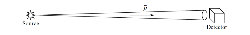
Figure 1: Illustration of variance in the direction of the virtual neutrino momenta due to a non-zero detector size.

Obviously, the picture has an approximate circular symmetry about the direction of momentum $\vec{p}$, which gives the factor $2\pi$ after the integration with respect to the azimuthal angle. Thus, the rules of the standard perturbative S-matrix theory should be modified in our case so as to include the factor $2\pi$ along with the delta function $\delta(P^{(1)}-P^{(1^{\prime})}-q-p)$, which fixes the 4-momentum $p$ of the intermediate neutrinos. Correspondingly, the final formula for the differential probability of the process under consideration looks like

$$\frac{{dW}}{{dp}} = \frac{1}{{2E^{(1)}2E^{(2)}}}\int{\frac{{d^{3}k}}{{\left({2\pi}\right)^{3}}}\frac{1}{{2k^{0}}}\frac{{d^{3}q}}{{\left({2\pi}\right)^{3}}}\frac{1}{{2q^{0}}}\frac{{d^{3}P^{(1^{\prime})}}}{{\left({2\pi}\right)^{3}}}\frac{1}{{2E^{(1^{\prime})}}}\frac{{d^{3}P^{(2^{\prime})}}}{{\left({2\pi}\right)^{3}}}\frac{1}{{2E^{(2^{\prime})}}}\left\langle{\left|M\right|^{2}}\right\rangle\times}$$ (20)

$$\times\left({2\pi}\right)^{4}\delta\left({P^{(1)}+P^{(2)}-P^{(1^{\prime})}-P^{(2^{\prime})}-q-k}\right)2\pi\delta\left({P^{(1)}-P^{(1^{\prime})}-q-p}\right),$$

which eliminates the contradiction and provides the consistent result: $\left.{\frac{{dW}}{{dp}}}\right|_{L=0}=\frac{{dW_{1}}}{{d\vec{p}}}W_{2}$.

In the approximation of massless neutrinos $\frac{{dW_{1}}}{{d\vec{p}}}$ coincides with the neutrino probability flux and $W_{2}$ coincides with the cross section of the scattering process of a massless fermion on nucleus 2. Thus, we have obtained that the probability of detecting an electron is equal to the probability of the neutrino production in the source multiplied by the probability of the neutrino interaction in the detector and the standard distance-dependent electron or neutrino survival probability, i.e. we have actually exactly reproduced the result of the standard approach to neutrino oscillations in the framework of QFT without making use of the neutrino flavor states. It is necessary to note that this result differs from the results of papers [4, 5, 6, 7] using the standard perturbative S-matrix theory, because all these papers reproduce the result of the standard approach with various corrections. If nuclei 1 in the source have a momentum distribution, the total neutrino probability flux can be obtained by performing the average of $\frac{{dW_{1}}}{{d\vec{p}}}$ over the momentum distribution of nucleus 1, and the number of events in the detector per unit time can be found by integrating the corresponding differential probability $\frac{{dW}}{{dp}}$ and the densities of nuclei 1 and nuclei 2 over the volumes of the neutrino source and detector.

The rules for calculating the probabilities of neutrino oscillation processes passing at finite distances and finite time intervals were suggested by the factorized structure of their squared amplitudes arising due to the extremely small neutrino masses. However, we believe that these rules can be used for calculating the probabilities of any processes passing at finite distances and finite time intervals. In particular, they can also be used for calculating the probabilities of oscillation processes with neutral kaons, where the differential probability of the processes factorizes exactly like in formula (17) due to a simpler structure of the amplitude of such processes in the case of scalar particles.

3 Oscillations in experiments with neutrino detection by neutral-current and charged-current interactions

Now we consider the case, where the neutrinos are produced in the charged-current interaction with nuclei and detected in both neutral-current and charged-current interactions with electrons, as it is done in the Kamiokande experiment. The corresponding processes are described by the following Feynman diagrams:

It is clear that in calculating the amplitude of the process the contribution of diagram (22) should be taken with all three neutrino mass eigenstates, i.e. $k=1,2,3.$ Since only the final electron is registered experimentally, the probabilities of the processes with different final neutrino states should be summed up to give the probability of registering an electron.

Now let us denote the particle momenta as follows: the momentum of the positron is $q$, the momentum of the virtual neutrinos is $p_{n}$, the momentum of the outgoing electron is $k$, the momentum of the incoming electron is $k_{1}$ and the momentum of the outgoing neutrino is $k_{2}$. Again we use the approximation of Fermi’s interaction and take time-dependent propagator (7) keeping the neutrino masses only in the exponential. Then the amplitude corresponding to diagram (21) in the momentum representation looks like

$$M_{nc}^{(i)} = i\frac{{G_{F}^{\,2}}}{4p_{n}^{0}}\,{U_{1i}^{*}}e^{-i\frac{{m_{i}^{2}-p_{n}^{2}}}{{2{p^{\,0}_{n}}}}T}\,\bar{\nu}_{i}\left(k_{2}\right)\gamma^{\mu}\left({1-\gamma^{5}}\right)\hat{p}_{n}\gamma^{\rho}\left({1-\gamma^{5}}\right)v\left(q\right)j_{\rho}\times$$

$$\times\left[\left(-\frac{1}{2}+\sin^{2}\theta_{W}\right)\bar{u}\left(k\right)\gamma_{\mu}(1-\gamma^{5})u\left(k_{1}\right)+\sin^{2}\theta_{W}\bar{u}\left(k\right)\gamma_{\mu}(1+\gamma^{5})u\left(k_{1}\right)\right].$$

Similarly, the sum over $k$ of the amplitudes corresponding to diagram (22) can be written out to be

$$M_{cc}^{(i)} = -i\frac{{G_{F}^{\,2}}}{4{p_{n}^{0}}}\,{U_{1i}^{*}}\left(\sum\limits_{k=1}^{3}{\left|{U_{1k}}\right|^{2}}e^{-i\frac{{m_{i}^{2}-p_{n}^{2}}}{{2{p^{\,0}_{n}}}}T}\right)\bar{u}\left(k\right)\gamma^{\mu}(1-\gamma^{5})\hat{p}_{n}\gamma^{\rho}\left({1-\gamma^{5}}\right)v\left(q\right)j_{\rho}\times$$ (24)

$$\times\bar{\nu}_{i}\left(k_{2}\right)\gamma_{\mu}(1-\gamma^{5})u\left(k_{1}\right).$$

Next it is convenient to use the Fierz identity, which transposes the spinors $\bar{u}\left(k\right)$ and $\bar{\nu}_{i}\left(k_{2}\right)$ in the amplitude $M_{cc}^{(i)}$ and makes this amplitude look similar to $M_{nc}^{(i)}$, and to introduce the following notations for the time-dependent factors:

$$A_{i}={U_{1i}^{*}}e^{-i\frac{{m_{i}^{2}-p_{n}^{2}}}{{2{p^{\,0}_{n}}}}T},\quad B_{i}={U_{1i}^{*}}\left(\sum\limits_{k=1}^{3}{\left|{U_{1k}}\right|^{2}}e^{-i\frac{{m_{i}^{2}-p_{n}^{2}}}{{2{p^{\,0}_{n}}}}T}\right).$$ (25)

Then the total amplitude of the process with neutrino $\nu_{i}$ in the final state, which is the sum of the amplitudes $M_{nc}^{(i)}$ and $M_{cc}^{(i)}$, can be represented as follows:

$$M_{tot}^{(i)}=i\frac{{G_{F}^{\,2}}}{4p_{n}^{\,0}}\,\bar{\nu}_{i}\left(k_{2}\right)\gamma^{\mu}\left({1-\gamma^{5}}\right)\hat{p}_{n}\gamma^{\rho}\left({1-\gamma^{5}}\right)v\left(q\right)j_{\rho}\times\phantom{aaaaaaaaaaaaaaaaaaaaaaaaaaaaaa}$$ (26)

$$\times\left[\left(B_{i}+A_{i}\left(-\frac{1}{2}+\sin^{2}\theta_{W}\right)\right)\bar{u}\left(k\right)\gamma_{\mu}(1-\gamma^{5})u\left(k_{1}\right)+A_{i}\sin^{2}\theta_{W}\bar{u}\left(k\right)\gamma_{\mu}(1+\gamma^{5})u\left(k_{1}\right)\right].$$

Now we have to calculate the squared amplitude, averaged with respect to the polarizations of the incoming nucleus and particles and summed over the polarizations of the outgoing nucleus and particles. Similar to the case of the neutrino detection in charged-current interaction, in the approximation $p_{n}^{2}=0$ the squared amplitude factorizes as follows:

$$\left\langle{\left|M_{tot}^{(i)}\right|^{2}}\right\rangle = \left\langle{\left|M_{1}\right|^{2}}\right\rangle\left\langle{\left|M_{2}^{(i)}\right|^{2}}\right\rangle\frac{{1}}{{4(p_{n}^{\,0})^{2}}},$$ (27)

$$\left\langle{\left|M_{1}\right|^{2}}\right\rangle = 4G_{F}^{\,2}\left(-{g^{\mu\nu}\left({p_{n}q}\right)+\left({p_{n}^{\mu}q^{\nu}+q^{\mu}p_{n}^{\nu}}\right)+i\varepsilon^{\mu\nu\alpha\beta}p_{n\alpha}q_{\beta}}\right)W_{\mu\nu}^{(1)},$$ (28)

$$\left\langle{\left|M_{2}^{(i)}\right|^{2}}\right\rangle = 64G_{F}^{\,2}\left[\left|B_{i}+A_{i}\left(-\frac{1}{2}+\sin^{2}\theta_{W}\right)\right|^{2}(p_{n}k_{1})^{2}+\left|A_{i}\right|^{2}\sin^{4}\theta_{W}(p_{n}k)^{2}-\right.$$ (29)

$$-\sin^{2}\theta_{W}Re\left(\left(B_{i}+A_{i}\left(-\frac{1}{2}+\sin^{2}\theta_{W}\right)\right)A_{i}^{*}\right)(p_{n}k_{2})m^{2}\Bigg{]}.$$

Here $\left\langle{\left|M_{1}\right|^{2}}\right\rangle$ is the squared amplitude of the decay process of nucleus $1$ into nucleus $1^{\prime}$, positron and a massless fermion, $W_{\mu\nu}^{(1)}$ denoting the corresponding averaged product of the matrix elements of the charged weak hadron current, and $\left\langle{\left|M_{2}^{(i)}\right|^{2}}\right\rangle$ is the squared amplitude of the scattering process of a massless fermion and the incoming electron.

As we have found in the previous section for the case of neutrino registration in charged-current interaction, to obtain the differential probability of the process we have to multiply the amplitude $\left\langle{\left|M_{tot}^{(i)}\right|^{2}}\right\rangle$ by the delta function of energy-momentum conservation $(2\pi)^{4}\delta(P^{(1)}+k_{1}-P^{(1^{\prime})}-q-k-k_{2})$ and by the delta function $2\pi\delta(P^{(1)}-P^{(1^{\prime})}-q-p)$ that selects the momentum of the virtual neutrinos, substitute $p$ instead of $p_{n}$ in it and to integrate with respect to the momenta of the outgoing particles and nucleus. This gives

$$\frac{dW^{(i)}}{dp} = \frac{dW_{1}}{d\vec{p}}\,W_{2}^{(i)},$$ (30)

$$\frac{dW_{1}}{d\vec{p}} = \int\frac{\left\langle{\left|M_{1}\right|^{2}}\right\rangle}{{2E^{(1)}}}(2\pi)^{4}\delta\left({P^{(1)}-P^{(1^{\prime})}-q-p}\right)\frac{{d^{3}q}}{{\left({2\pi}\right)^{3}}{2q^{0}}}\frac{{d^{3}P^{(1^{\prime})}}}{{\left({2\pi}\right)^{3}}{2E^{(1^{\prime})}}}\frac{1}{{\left({2\pi}\right)^{3}}{2p^{\,0}}},$$ (31)

$$W_{2}^{(i)} = \int\frac{\left\langle{\left|M_{2}^{(i)}\right|^{2}}\right\rangle}{2p^{\,0}2k_{1}^{0}}(2\pi)^{4}\delta(k_{1}+p-k-k_{2})\frac{{d^{3}k}}{{\left({2\pi}\right)^{3}}{2k^{0}}}\frac{{d^{3}k_{2}}}{{\left({2\pi}\right)^{3}}{2k_{2}^{0}}}.$$ (32)

Formula (31) means that $\frac{dW_{1}}{d\vec{p}}$ is the differential decay probability of nucleus 1 into nucleus $1^{\prime}$, positron and a massless neutral fermion with fixed momentum $\vec{p}$. In fact, this is the sum of the differential decay probabilities of nucleus 1 into nucleus $1^{\prime}$, positron and all the three neutrino mass eigenstates $\nu_{i}$ with fixed momentum $\vec{p}$ taken in the approximation of zero neutrino masses. Similarly, in accordance with formula (32), the probability $W_{2}^{(i)}$ is the probability of the process of scattering of a massless neutral fermion and electron with the production of electron and the neutrino mass eigenstate $\nu_{i}$ in the final state. Obviously, this probability is the sum of the probabilities of the processes of scattering of electron and all the three neutrino mass eigenstates with the production of electron and the neutrino mass eigenstate $\nu_{i}$ in the final state.

To obtain the probability of finding an electron in the final state we have to sum the probability $\frac{dW^{(i)}}{dp}$ over $i=1,2,3$. Obviously, this reduces to summing over $i$ the squared amplitude $\left\langle{\left|M_{2}^{(i)}\right|^{2}}\right\rangle$, because only this amplitude depends on $i$.

Since now the virtual neutrinos have fixed momentum $p$, we can replace $T$ by $Lp^{\,0}/|\vec{p}|$ in all the subsequent formulas. Then the definition of the time-dependent factors $A_{i}$ and $B_{i}$ in (25) leads to the following expressions for their absolute values and products:

$$\left|A_{i}\right|^{2} = \left|U_{1i}\right|^{2},$$ (33)

$$\left|B_{i}\right|^{2} = \left|U_{1i}\right|^{2}\left[{1-4\sum\limits_{\scriptstyle k,l=1\hfill\atop\scriptstyle k<l\hfill}^{3}{\left|{U_{1k}}\right|^{2}\left|{U_{1l}}\right|^{2}\sin^{2}\left({\frac{{m_{k}^{2}-m_{l}^{2}}}{{4\left|{\vec{p}}\right|}}L}\right)}}\right],$$ (34)

$$Re\left(A_{i}B_{i}^{*}\right) = \left|U_{1i}\right|^{2}\sum\limits_{\scriptstyle k=1}^{3}\left|{U_{1k}}\right|^{2}\cos^{2}\left({\frac{{m_{k}^{2}-m_{i}^{2}}}{{4\left|{\vec{p}}\right|}}L}\right).$$ (35)

Substituting these expressions into formula (29) and summing over $i$, we get

$$\sum\limits_{\scriptstyle i=1}^{3}\left\langle{\left|M_{2}^{(i)}\right|^{2}}\right\rangle=64G_{F}^{\,2}\Bigg{[}\sin^{4}\theta_{W}(pk)^{2}+$$ (36)

$$+\left(\left(\frac{1}{2}+\sin^{2}\theta_{W}\right)^{2}-8\sin^{2}\theta_{W}\sum\limits_{\scriptstyle k,l=1\hfill\atop\scriptstyle k<l\hfill}^{3}{\left|{U_{1k}}\right|^{2}\left|{U_{1l}}\right|^{2}\sin^{2}\left({\frac{{m_{k}^{2}-m_{l}^{2}}}{{4\left|{\vec{p}}\right|}}L}\right)}\right)(pk_{1})^{2}-$$

$$\left.-\left(\sin^{2}\theta_{W}\left(\frac{1}{2}+\sin^{2}\theta_{W}\right)-4\sin^{2}\theta_{W}\sum\limits_{\scriptstyle k,l=1\hfill\atop\scriptstyle k<l\hfill}^{3}\left|{U_{1k}}\right|^{2}\left|{U_{1l}}\right|^{2}\sin^{2}\left({\frac{{m_{k}^{2}-m_{l}^{2}}}{{4\left|{\vec{p}}\right|}}L}\right)\right)(pk_{2})m^{2}\right].$$

Next substituting this expression into formula (32) summed over $i$ and evaluating the integrals with the help of the formulas for neutrino-electron scattering kinematics presented in §16 of textbook [11], we arrive at the following result:

$$W_{2} = \frac{{G_{F}^{2}m}}{{2\pi}}\frac{{2\left|{\vec{p}}\right|^{2}}}{{2\left|{\vec{p}}\right|+m}}\left[{1-2\sin^{2}\theta_{W}\left({1+\frac{{2\left|{\vec{p}}\right|}}{{2\left|{\vec{p}}\right|+m}}}\right)+4\sin^{4}\theta_{W}\left({1+\frac{1}{3}\left({\frac{{2\left|{\vec{p}}\right|}}{{2\left|{\vec{p}}\right|+m}}}\right)^{2}}\right)+}\right.$$ (37)

$$\left.{+4\sin^{2}\theta_{W}\left({1+\frac{{2\left|{\vec{p}}\right|}}{{2\left|{\vec{p}}\right|+m}}}\right)\left({1-4\sum\limits_{\scriptstyle k,l=1\hfill\atop\scriptstyle k<l\hfill}^{3}{\left|{U_{1k}}\right|^{2}\left|{U_{1l}}\right|^{2}\sin^{2}\left({\frac{{m_{k}^{2}-m_{l}^{2}}}{{4\left|{\vec{p}}\right|}}L}\right)}}\right)}\right].$$

We see that in the case, where the neutrinos are produced in the charged-current interaction with nuclei and detected in both neutral-current and charged-current interactions with electrons, the situation is different from the case, where neutrinos are detected in charged-current interactions. The same situation takes place in the standard approach and the formula for $W_{2}$ exactly coincides with the expression $P_{\nu_{e}\to\nu_{e}}\sigma_{\nu_{e}e}+(1-P_{\nu_{e}\to\nu_{e}})\sigma_{\nu_{\mu}e}$, which one expects for this quantity in the standard approach.

4 Conclusion

In the present paper we have shown that it is possible to calculate consistently neutrino oscillation processes in a quantum field-theoretical approach within the framework of the SM minimally extended by the right neutrino singlets. To this end we have adapted the standard formalism of perturbative S-matrix for calculating the amplitudes of the processes passing at finite distances and finite time intervals by modifying the Feynman propagator. The developed approach is physically transparent and, unlike the standard one, has the advantage of not violating the energy-momentum conservation. In its framework, the calculation of amplitudes is carried out in the way that is most similar to the one used in the usual perturbative S-matrix formalism, which is much simpler than in papers [4, 6], where an approach based on the use of wave packets and the standard Feynman propagators for describing the motion of virtual neutrinos has been developed.

The application of this modified formalism to describing the neutrino oscillation processes with neutrino detection by charged-current and neutral-current interactions with electrons showed that the standard results can be easily and consistently obtained using only the mass eigenstates of these particles. This differs the developed approach from the approaches of papers [4, 5, 6, 7], where the results of describing the neutrino oscillation processes with neutrino detection by charged-current interaction include corrections to the results of the standard approach coming from the wave packet structure of the initial particle states.

Acknowledgments
The authors are grateful to E. Boos, A. Lobanov and M. Smolyakov for reading the manuscript and making important comments and to L. Slad for useful discussions. Analytical calculations of the amplitudes have been carried out with the help of the COMPHEP and REDUCE packages. The work was supported by grant NSh-7989.2016.2 of the President of Russian Federation.

References

- [1] C. Giunti and C. W. Kim, Oxford, UK: Univ. Pr. (2007) 710 p.
- [2] S. Bilenky, Lect. Notes Phys. 817 (2010) 1.
- [3] K. Nakamura and S.T. Petcov, in: K.A. Olive et al. (Particle Data Group), Chin. Phys. C 38, 090001 (2014).
- [4] C. Giunti, C. W. Kim, J. A. Lee and U. W. Lee, Phys. Rev. D 48 (1993) 4310.
- [5] W. Grimus and P. Stockinger, Phys. Rev. D 54 (1996) 3414.
- [6] D. V. Naumov and V. A. Naumov, J. Phys. G 37 (2010) 105014 [arXiv:1008.0306 [hep-ph]].
- [7] A. E. Lobanov, arXiv:1507.01256 [hep-ph].
- [8] I. P. Volobuev, arXiv:1703.08070 [hep-ph].
- [9] R. P. Feynman, Phys. Rev. 76 (1949) 769.
- [10] N.N. Bogoliubov and D.V. Shirkov, ”Introduction to the theory of quantized fields”, 3d edition, John Wiley & Sons, New York Chichester Brisbane Toronto, 1980.
- [11] L. B. Okun, ”Leptons and Quarks”, New York: North Holland, 1984.