B-CNN: Branch Convolutional Neural Network for Hierarchical Classification

Abstract

Convolutional Neural Network (CNN) image classifiers are traditionally designed to have sequential convolutional layers with a single output layer. This is based on the assumption that all target classes should be treated equally and exclusively. However, some classes can be more difficult to distinguish than others, and classes may be organized in a hierarchy of categories. At the same time, a CNN is designed to learn internal representations that abstract from the input data based on its hierarchical layered structure. So it is natural to ask if an inverse of this idea can be applied to learn a model that can predict over a classification hierarchy using multiple output layers in decreasing order of class abstraction. In this paper, we introduce a variant of the traditional CNN model named the Branch Convolutional Neural Network (B-CNN). A B-CNN model outputs multiple predictions ordered from coarse to fine along the concatenated convolutional layers corresponding to the hierarchical structure of the target classes, which can be regarded as a form of prior knowledge on the output. To learn with B-CNNs a novel training strategy, named the Branch Training strategy (BT-strategy), is introduced which balances the strictness of the prior with the freedom to adjust parameters on the output layers to minimize the loss. In this way we show that CNN based models can be forced to learn successively coarse to fine concepts in the internal layers at the output stage, and that hierarchical prior knowledge can be adopted to boost CNN models’ classification performance. Our models are evaluated to show that the B-CNN extensions improve over the corresponding baseline CNN on the benchmark datasets MNIST, CIFAR-10 and CIFAR-100.

1 Introduction

The traditional CNN based classification models are designed to be sequential and output the only prediction at the top of the models without any branching of the network at the outputs. This is because these models assume that all classes are equally difficult to distinguish and treat all of them exclusively. But in fact, the property of general-to-specific category ordering often exists between classes, e.g., cat and dog can usually be grouped as pet while chair and bed are furniture, and it is often easier to tell a cat apart from a bed than from a dog. This property indicates that classification can be done in a hierarchical way instead of treating all classes as arranged in a “flat” structure. When doing hierarchical classification, a classifier first knows an apple should be in the coarse category of fruit, then it can be classified at the finer level as an apple. One benefit of hierarchical classification is that the error can be restricted to a subcategory, which also means it should be more informative than flat classification. For example, a classifier may confuse an apple with an orange, but knows it should at least be fruit so won’t confuse it with, say, a red snooker ball.

CNN based models are naturally hierarchical. As Zeiler and Fergus present in [34], lower layers in CNN usually capture the low level features of an image such as basic shapes while higher layers are likely to extract high level features such as the face of a dog. As a consequence, a possible way to embed a hierarchy of classes into a CNN model is to output multiple predictions along the CNN layers as the data flow through, from coarse to fine. In this case, lower layers output coarser predictions while higher layers output finer predictions. Unlike traditional CNN models which do not capture the complexity of semantic labels in the real world, hierarchical classification models can do predictions in a more interpretable way and even boost the final classification as the hierarchical prior is a good guide to the classifier.

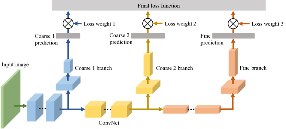
(a)

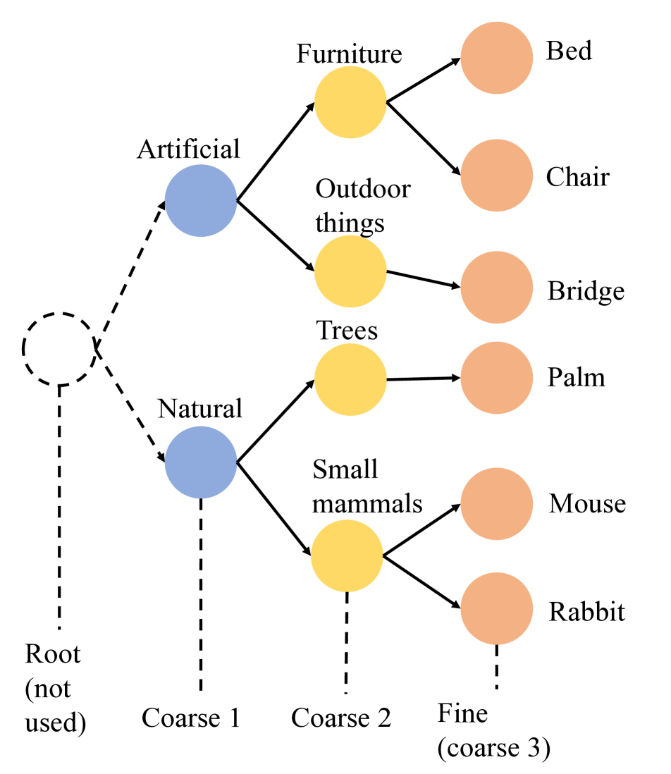
(b)

Figure 1: (a) Architecture of Branch Convolutional Neural Network (B-CNN). The network at the bottom can be an arbitrary ConvNet. There can be multiple branch networks and each of them outputs a coarse prediction. The final loss function is a weighted summation of all coarse losses. (b) A sample hierarchical label tree where classes are taken from CIFAR-100 dataset.

In this paper, we introduce a special CNN based model integrated with the prior knowledge of hierarchical category relations (https://github.com/zhuxinqimac/B-CNN). We name it Branch Convolutional Neural Network (B-CNN) as it contains several branch networks along the main convolution workflow to do predictions hierarchically. The architecture of B-CNN is shown in Figure 1(a). Our B-CNN model is inspired by the idea from [34] that each layer of a CNN contains the hierarchical nature of the features in the network. We exploit this property of CNN to combine it with the prior knowledge of class hierarchical structure to enforce the network to learn human understandable concepts in different layers.

Beside B-CNN, we also propose a novel training strategy which is tailored to our B-CNN models named Branch Training strategy (BT-strategy). When training a B-CNN model with BT-strategy, lower level parameters are activated and trained earlier than the higher level parameters. This idea is inspired by the vanishing gradient problem [11] and the step-by-step training method adopted by Simonyan and Zissermanto to train a deep ConvNet in [27]. BT-strategy can prevent the impact of vanishing gradient problem to an extent and boost the performance of a B-CNN model.

This paper’s major contributions are summarized below. First, we introduce a new CNN based model for hierarchical classification. Second, our work presents the possibility of embedding the semantic structure of target classes into a CNN model to demonstrate the interpretability of convolutional neural network. Third, we propose a novel training strategy tailored to B-CNN which can boost the classification accuracy. We validate our model and training strategy on MNIST, CIFAR-10 and CIFAR-100 datasets, showing significant empirical benefits.

2 Related Work

CNN based models have been successfully exploited in many computer vision tasks and the most successful one is image classification [16]. There are various techniques introduced to enhance CNN’s performance in the past literature. Simonyan and Zisserman show us that increasing the depth of a CNN model [27] within a boundary is likely to boost the classifier’s accuracy. In [34] and [26], a large number of filters has been adopted. Recently, there have been a vast amount of work to enhance the components of CNN such as novel types of activation functions [4, 8], the replacement of linear filter patches [20], pooling operation [18, 28, 33] and initialization strategies [23]. These attempts mainly focus on the potential weakness inside the existent CNN models and try to find a replacement or propose any strategy to improve it. Different from them, our B-CNN model is taking existent CNNs as building blocks, exploiting natural hierarchical property of CNN [34], and boosting performance with a tailored training strategy.

Exploiting hierarchical structure of object category has a long history [30]. In [14, 35], hierarchy in classes has been used to combine different models for better performance. The hierarchy of classes can either be predefined by human [21, 31, 35], or constructed automatically by top-down and bottom-up approaches [1, 19, 22, 25].

Combining tree structure prior with CNN models has drawn interest recently. Srivastava et al. [29] propose a method which benefits from CNN and tree-based prior when the training set is very small. They have shown that label tree prior can be used to transfer knowledge between classes and boost the performance when training examples are insufficient. But their method does not exploit the hierarchical nature within the layers which remains the whole CNN model a black box. Jia et al. [5] introduce a graph representation to capture the hierarchical and exclusive semantics between labels. They define a joint distribution of an assignment of all labels as a Conditional Random Field and use it to replace the traditional classifiers such as softmax on the top of a deep neural network. However their work still uses the network as a feature extractor and there is no attempt to exploit the hierarchical nature of CNN itself.

Zhicheng et al. [32] have made a significant contribution in discovering the possibility of combing the label tree and the hierarchical nature of CNN. In their work, classes are grouped as coarse categories and their HD-CNN model separates easy categories using a shared coarse classifier while distinguishing difficult classes using fine category classifiers. This model confirmed that the hierarchical property in CNN can be exploited. A potential problem of HD-CNN is that it requires the coarse and fine category components to be pretrained and followed by a fine-tune procedure which is quite time-consuming. HD-CNN also only uses one coarse category which is not scalable because there may be far more than one levels of coarse categories in a hierarchical label tree.

More recently work has combined deep learning with probabilistic graphical models such as MRFs, CRFs, etc. (e.g. [3]), but this either requires a two-stage training process, or new methods of training the combined model, which is not as straightforward as training in a B-CNN. An end-to-end approach is the Structured Prediction Energy Networks of [2] but this is not based on CNNs.

The vanishing gradient problem [11] has existed in neural networks for a long time and various methods have been proposed to handle it. Rectified linear units (ReLU) have been successfully adopted in deep neural networks [7] as the activation function. LSTM models use forget gates to solve the vanishing gradient issue in RNNs [6, 12]. Recently, residual neural networks (ResNets) eliminate this problem by adding identity shortcut connections between three layer chunks in ConvNets [9]. Our BT-strategy relieves this issue in B-CNNs by shifting the loss weights of different coarse level outputs, ultimately making it converge to a traditional CNN classifier.

3 Model Description

3.1 Branch Convolutional Neural Network

The overview architecture of Branch Convolutional Neural Network (B-CNN) is shown in Figure 1(a) and a corresponding label tree is in Figure 1(b). In the label tree, fine labels are target classes and are always provided by the classification task. They are presented as leaves and clustered into coarse categories which can be manually constructed or generated by unsupervised methods. More general categories can be used, e.g., coarse 1 level in Figure 1(b) is a super-level of coarse 2. In order not to cause ambiguity, we use level to refer to the different layers in the label tree, layer as the layers in the neural network and branch as the branch output nets of B-CNN.

A B-CNN model uses existent CNN components as building blocks to construct a network with internal output branches. The network shown at the bottom in Figure 1(a) is a traditional convolutional neural network. It can be an arbitrary ConvNet with multiple layers. The middle part in Figure 1(a) shows the output branch networks of a B-CNN. Each branch net produces a prediction on the corresponding level in the label tree (Figure 1(b), shown in same color). On the top of each branch, fully connected layers and a softmax layer are used to produce the output in one-hot representation. Branch nets can consist of ConvNets and fully connected neural networks. But for simplicity, in our experiments, we only use fully connected neural networks as our branch nets.

When doing classification, a B-CNN model outputs as many predictions as the levels the corresponding label tree has. For example, considering the label tree shown in Figure 1(b), an image of a mouse will contain a hierarchical label of [natural, small mammals, mouse]. When the image is fed into B-CNN, the network will output three corresponding predictions as the data flow through and each level’s loss will contribute to the final loss function (introduced in 3.2) base on the loss weights distribution (introduced in 3.3).

3.2 Loss Function

The loss function of B-CNN is a weighted summation of all coarse and find prediction losses. The loss function is defined in (1):

$$L_{i}=\sum_{k=1}^{K}-A_{k}\log{\bigg{(}\frac{e^{f_{y_{i}}^{k}}}{\sum_{j}e^{f_{j}^{k}}}\bigg{)}}$$ (1)

where $i$ denotes the $i^{th}$ sample in the mini-batch. $K$ is the number of coarse levels in the label tree and $A_{k}$ is the loss weight (introduced in 3.3) of $k^{th}$ level contributing to the loss function. The term $-\log{\bigg{(}\frac{e^{f_{y_{i}}^{k}}}{\sum_{j}e^{f_{j}^{k}}}\bigg{)}}$ is the cross-entropy loss of the $i^{th}$ sample on the $k^{th}$ level in the label tree and we use $f_{j}$ to denote the $j^{th}$ element in the vector $f$ of class scores, outputted by the last layer of the model.

The loss function takes all levels’ loss into account to make sure the structure prior can play a role of internal guide to the whole model and make it easier to flow the gradients back to the shallow layers.

3.3 Loss Weight

Value $A_{k}$ in (1) is the loss weight of each branch network in B-CNN. This value defines how much contribution a level makes to the final loss function. Although only relative value matters how the loss function works, we use a standard representation in our experiments that each $A_{k}$ should be a value between 0 and 1 (both included) and their summation should be 1, e.g., we use loss weights [0.1, 0.1, 0.8] for a three level label tree instead of [1, 1, 8].

This definition of loss weight also makes the B-CNN a super model of traditional CNN. For instance, for a three-branch B-CNN (corresponding to a three level label tree), when loss weights are fixed to [0, 0, 1], the B-CNN model converges to a traditional CNN model with only the last output branch trainable. With loss weights of [1, 0, 0], the B-CNN will only activate the former part of the whole network remaining the two higher levels untrained. The distribution of loss weights also indicates the importance of each level, e.g., loss weights of [0.98, 0.01, 0.01] mean the model values the low level feature extraction but also want to train a little bit of the deep layers, and in our experiments, we usually use this assignment as the initialization of our loss weights.

3.4 Branch Training Strategy

Our Branch Training strategy (BT-strategy) exploits the potential of loss weights distribution to achieve an end-to-end training procedure with low impact of vanishing gradient problem [11]. BT-strategy modifies the loss weights distribution while training a B-CNN model, e.g., for a two level classification, the initial loss weights can be assigned as [0.9, 0.1], and then they can be changed to [0.2, 0.8] after 50 epochs.

The greatest value in a loss weights assignment can be regarded as a “focus”, e.g., 0.5 is the focus of [0.2, 0.3, 0.5]. A “focus” is not necessary in a distribution as all levels can be equally important. However, in our implementation, we usually set a “focus” to explicitly tell the classifier to learn this level with more efforts. Usually, the “focus” of a distribution will shift from lower level to higher level (from coarse to fine). This procedure requires the classifier to extract lower features first with coarse instructions and fine tune parameters with fine instructions later. It to an extent prevents the vanishing gradient problem which would make the updates to parameters on lower layers very difficult when the network is very deep.

4 Experiments

4.1 Overview

In our experiments, first we want to see what our B-CNN is doing when handling a hierarchical classification task (in 4.2). Then we compare the performance of B-CNN models with their corresponding baseline traditional CNN models (defined in 4.3) on benchmark datasets MNIST (in 4.4), CIFAR-10 (in 4.5) and CIFAR-100 (in 4.6). Finally we analyze our experiment results in 4.7.

In all experiments, we use stochastic gradient decent(SGD) as our optimizer with momentum set to be 0.9. All of our models are trained on Intel(R) Xeon(R) CPU E5-2637 v4, and the number of training epochs are limited to less than 80 on all datasets. This setting may result in immaturely trained models, but as we focus on the comparison between our B-CNN models and the baseline models instead of beating the current best models on these datasets, it is enough to show the idea of this paper. In our implementation, all models are trained without data augmentation and no ensemble methods are adopted.

4.2 Hierarchical Classification

In this section, we choose a B-CNN model to show its behavior during training. The model is constructed with the baseline model B (second column in Table 1) and its corresponding branch networks (second column in Table 2). The total number of training epochs is limited to 60. The learning rate is initialized with 0.003 and changes to 0.0005 at epoch 42 and 0.0001 after 52 epochs. The loss weights of the 3 branches are set to be [0.33, 0.33, 0.34] to show their even importance.

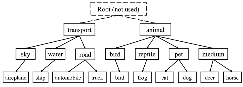
Figure 2: A manually constructed label tree for CIFAR-10 dataset.

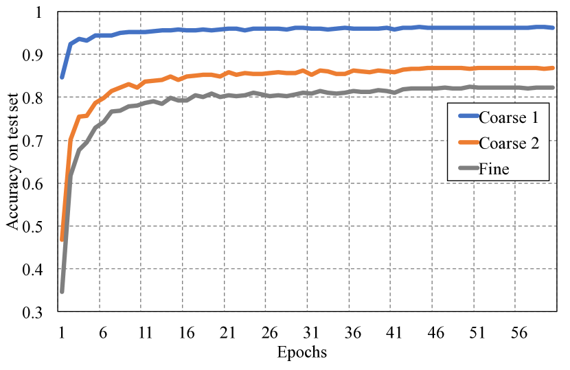
Figure 3: Accuracy of each level based on the constructed label tree for CIFAR-10 dataset in Figure 2.

The dataset used in this section is CIFAR-10. The CIFAR-10 dataset [15] consists of 10 classes of $32\times 32$ RGB images with 50,000 training and 10,000 testing examples in total. Because there is no official label tree for this dataset, we manually construct one with natural categories of the classes, e.g., cat and dog are clustered as pet while deer and horse are grouped as medium animal. The coarsest level consists of transport and animal categories. The constructed label tree is shown in Figure 2. The model will output three accuracy results for coarse 1, coarse 2 and fine levels based on the label tree.

The results are shown in Figure 3. The coarse 1 level gets the highest accuracy and is trained fastest, followed by coarse 2 level and fine level. This is very reasonable as the coarse 1 level is the easiest one (just need to distinguish transport and animal) and the corresponding network is the most shallow one. On the contrary, the fine level, which is to distinguish all 10 classes, is the most difficult task among the three. Levels reach accuracy of 96.26%, 86.74% and 82.19% respectively, meaning the layers before coarse 1 branch have learned enough features which can tell an image of transport from animal with high confidence. This confirms the usefulness of B-CNN to do a hierarchical classification and the results are consistent with our common sense.

4.3 Baseline Configuration

In the following sections we will compare B-CNN models with their corresponding baseline models on benchmark datasets.

The chosen baseline configurations roughly follow the construction scheme proposed by Simonyan and Zisserman’s [27], using $3\times 3$ patch size filters with stride fixed to 1 pixel. ReLUs are used as activation layers and max-pooling is performed over a $2\times 2$ pixel window with stride of 2. Dropout [10] regularization is adopted between fully connected layers to prevent overfitting. We also use Batch Normalization [13] at each layer for easier initialization and training.

Specific configurations of three baseline models are shown in Table 1. Base C model is VGG16 [27] and because this network is too deep to train from scratch without GPU, we initialize the parameters of this model with pre-trained parameters on ImageNet [24] and fine tune it on CIFAR-10 and CIFAR-100 datasets.

The corresponding B-CNN models are just an assembling of Table 1 and Table 2. Let’s take B-CNN B as an example, B-CNN B is constructed with Base B network in Table 1 and Branches of B in Table 2, where symbol * shows the conjunction. In Table 2, the block [Flatten, FC-256, FC-256, FC-$c_{B1}$] is the coarse 1 branch shown in Figure 1(a) and [Flatten, FC-512, FC-512, FC-$c_{B2}$] is the coarse 2 branch. The last block of Base B in Table 1, [Flatten, FC-1024, FC-1024, FC-$x$], is the fine branch in Figure 1(a), and the rest part of Base B is the ConvNet at the bottom in Figure 1(a).

Base A	Base B	Base C
$28\times 28\times 1$ image	$32\times 32\times 3$ image
conv3-32	(conv3-64)×2	(conv3-64)×2
maxpool-2 *	maxpool-2	maxpool-2
conv3-64	(conv3-128)×2	(conv3-128)×2
	maxpool-2 *	maxpool-2
conv3-64	(conv3-256)×2	(conv3-256)×3
	maxpool-2 **	maxpool-2 *
	(conv3-512)×2	(conv3-512)×3
maxpool-2	maxpool-2	maxpool-2 **
		(conv3-512)×3
Flatten
FC-128	FC-1024	FC-4096
FC-10	FC-1024	FC-4096
	FC-$x$	FC-$x$
softmax layer

Table 1: Baseline networks. Base A model is tested on MNIST dataset. Both B and C are tested on CIFAR-10 and CIFAR-100. The $x$ in last ConvNet layer of Base B and C can be replaced by 10 or 100. Base C model is VGG16 [27] without last max-pooling layer because images in CIFAR datasets are very small. Symbol * means there is a branch network attached to that layer for corresponding B-CNN models, and the specific branch configurations are shown in Table 2.

Branches of A	Branches of B	Branches of C
* Flatten
FC-64	FC-256	FC-512
FC-$c_{A1}$	FC-256	FC-512
	FC-$c_{B1}$	FC-$c_{C1}$
	** Flatten
	FC-512	FC-1024
	FC-512	FC-1024
	FC-$c_{B2}$	FC-$c_{C2}$

Table 2: Branch networks for each B-CNN model. Symbol * means this branch is connected to the layer with the same * in Table 1, e.g., there is a branch of network [Flatten, FC-64, FC-$c_{A1}$] after the first maxpooling layer in B-CNN A model.

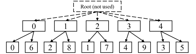
Figure 4: A manually constructed label tree for MNIST dataset.

4.4 MNIST

The MNIST [17] dataset is composed of gray-scale hand written digits 0-9 which are $28\times 28$ in size, containing 60,000 training and 10,000 testing examples.

The baseline model tested on this dataset is Base A in Table 1. The corresponding B-CNN model is constructed with the exact same configuration but added with a branch output network after the first maxpooling layer to do the coarse prediction (first column in Table 2). Because the MNIST dataset does not provide official label tree, we manually construct one with common sense, e.g., it is reasonable to say 0 and 6 are similar. The manually constructed label tree is in Figure 4.

The accuracy of both models are shown in Figure 5. Both models’ initial learning rates are set to be 0.01 and decrease to 0.002 after 28 epochs and 0.0004 after 35 epochs. For B-CNN model, the loss weights of the two output branches will change because of the BT-strategy. Specifically, loss weights pair [$A_{1},A_{2}$] is set to be: epoch 1: [0.98, 0.02], epoch 12: [0.60, 0.40], epoch 18: [0.20, 0.80], epoch 22: [0, 1]. When [$A_{1},A_{2}$] changes to [0, 1], B-CNN is converged to the traditional CNN (baseline model). As we see, the B-CNN model is trained much slower than the baseline at the beginning (baseline reaches 99% at epoch 4 while B-CNN only gets 92%), but it speeds up significantly at the epoch of 12. This phenomenon is caused by the change of loss weighs distribution. At the beginning, low contribution to the loss function makes the fine level prediction less important. After the loss weights change, the focus of the loss function has been shifted to the fine level and force the model to learn more specific features much faster than it did earlier.

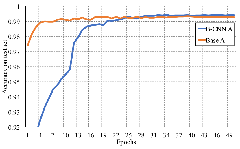
Figure 5: Comparison on test set between baseline model A and its corresponding B-CNN model A on MNIST dataset.

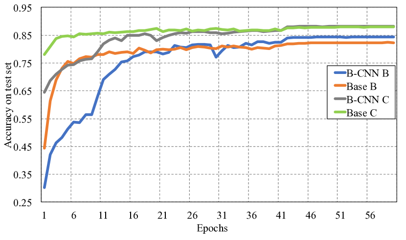
Figure 6: Comparison on test set between baseline models and their corresponding B-CNN models on CIFAR-10 dataset.

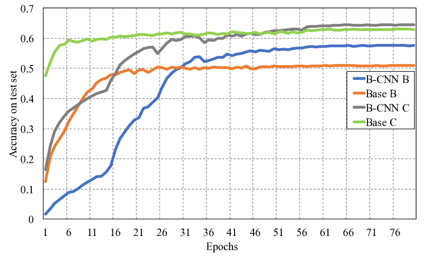
Figure 7: Comparison on test set between baseline models and their corresponding B-CNN models on CIFAR-100 dataset.

Models	MNIST	CIFAR-10	CIFAR-100
Base A	99.27%	-	-
B-CNN A	99.40%	-	-
Base B	-	82.35%	51.00%
B-CNN B	-	84.41%	57.59%
Base C	-	87.96%	62.92%
B-CNN C	-	88.22%	64.42%

Table 3: Performance of each model on MNIST, CIFAR-10 and CIFAR-100 test sets.

4.5 CIFAR-10

The CIFAR-10 dataset [15] consists of 10 classes of $32\times 32$ RGB images with 50,000 training and 10,000 testing examples in total.

The baseline model tested on this dataset is Base B and Base C. Same as MNIST, the corresponding B-CNN models use the exact same configuration as baseline models with two additional branches to output extra coarse predictions (second and third columns in Table 2). The corresponding label tree used in this experiment is the same one used in 4.2 (shown in Figure 2).

For model B, both models’ learning rates are initialized to be 0.003 and decease to 0.0005 after 42 epochs and 0.0001 after 52 epochs. For B-CNN model, the change of loss weights follows the scheme: epoch 1: [0.98, 0.01, 0.01], epoch 10: [0.10, 0.80, 0.10], epoch 20: [0.1, 0.2, 0.7], epoch 30: [0, 0, 1].

For model C, we use the pre-trained parameters of VGG16 on ImageNet dataset to initialize both the baseline and B-CNN models then fine tune them on CIFAR-10 dataset, using the same training procedure for model B.

The result is shown in Table 3 and Figure 6. The baseline model B gets an accuracy of 82.35% after 60 epochs and the B-CNN model B reaches 84.41%. For B-CNN model B, the loss weight of the fine-level loss increases at epoch 10, so there is an obvious tendency shift at that point. As we see, the new growth trend is much steeper than the old one, which indicates that the network is putting more effort to learn more specific features. For baseline C and B-CNN C, the training procedure is very similar to models of B, but the final accuracy gap between B-CNN and baseline is smaller. We presume the different initialization caused this difference as for B the parameters are initialized randomly while for C they are initialized with pre-trained parameters, which makes the BT-strategy less important.

4.6 CIFAR-100

The CIFAR-100 dataset [15] is just like CIFAR-10 with $32\times 32$ images, except that it has 100 classes containing 600 images each. The 100 fine classes in the CIFAR-100 are grouped into 20 coarse classes. In this case, we also manually group the provided 20 superclasses into 8 coarser classes as a more informative prior. The corresponding B-CNN models are with same configuration but extra branches shown in second and third columns in Table 2.

The training procedures on CIFAR-100 are very similar to the ones on CIFAR-10 except the learning rate and loss weights which are determined by cross validation. The learning rates of all models trained on CIFAR-100 are initialized as 0.001 and drop to 0.0002 at epoch 55 and 0.00005 after epoch 70. The loss weights modification scheme for B-CNNs are: epoch 1: [0.98, 0.01, 0.01], epoch 15: [0.10, 0.80, 0.10], epoch 25: [0.1, 0.2, 0.7], epoch 35: [0, 0, 1]. Same as on CIFAR-10, the type C models are initialized with existent VGG16 parameters pre-trained on ImageNet dataset.

The performance of models trained on CIFAR-100 are shown in Table 3 and Figure 7. For model B, the baseline model gets 51.00% accuracy while its corresponding B-CNN model reaches 57.59%. Though this model may not be fully trained as we limit the number of epochs to 80, it can be seen in Figure 7 that B-CNN model can reach high accuracy faster than the baseline model. The baseline model C and B-CNN model C get 62.92% and 64.42% accuracy respectively. Note that same as in CIFAR-10, the accuracy gap between baseline and B-CNN on model C is smaller than that on model B. This may be caused by the initialization of pre-trained parameters, which makes it much easier for the baseline model to fine tune weights.

4.7 Analysis

These experiments on three different datasets share many features. First the learning pattern of B-CNNs differs from traditional CNNs. There is an obvious acceleration of learning speed after the loss weights contribution shift in B-CNN models. This phenomenon confirms that using coarse level labels to learn low level features first is very useful to activate the shallow layers of a CNN model. In other words, our BT-strategy prevents B-CNNs from suffering the vanishing gradient problem. Second, B-CNN models consistently outperform their corresponding baseline models. This result is a convincing evidence that hierarchical nature of CNNs can be connected to the structure prior of target classes to strengthen the classifier. Third, B-CNN models are as simple as traditional CNNs. B-CNNs only use existent CNN components as building blocks and BT-strategy is achieved as easily as modifying learning rates. Forth, a good initialization may downgrade the benefit of B-CNN. When models are initialized with pre-trained parameters, the performance gap between B-CNN and baseline models is not that obvious. We presume it is because when pre-trained parameters are used, the low level features have already been successfully extracted so the benefit of BT-strategy is not very obvious.

5 Conclusion

In this paper, we introduced the Branch Convolutional Neural Network (B-CNN) which connects the hierarchical nature of CNNs and a structured prior on target classes. Compared with traditional CNN models, B-CNN can output multiple hierarchical predictions from coarse to fine, which is more informative and interpretable. We also introduce B-CNN’s tailored Branch Training strategy (BT-strategy) to force the model to learn low-level features at the beginning of training and converge later to traditional CNN classification. This strategy enables B-CNN models to utilize label trees as internal guides, and boosts performance significantly. The experiment results confirm the benefits of our model over the traditional CNN. For further work the possibility of learning with other structured outputs, such as linear chains or graphs, should be investigated.

References

- [1] H. Bannour and C. Hudelot. Hierarchical image annotation using semantic hierarchies. In Proceedings of the 21st ACM International Conference on Information and Knowledge Management, CIKM ’12, pages 2431–2434, New York, NY, USA, 2012. ACM.
- [2] D. Belanger and A. McCallum. Structured prediction energy networks. CoRR, abs/1511.06350, 2015.
- [3] L. Chen, G. Papandreou, I. Kokkinos, K. Murphy, and A. L. Yuille. Deeplab: Semantic image segmentation with deep convolutional nets, atrous convolution, and fully connected crfs. CoRR, abs/1606.00915, 2016.
- [4] D. Clevert, T. Unterthiner, and S. Hochreiter. Fast and accurate deep network learning by exponential linear units (elus). CoRR, abs/1511.07289, 2015.
- [5] J. Deng, N. Ding, Y. Jia, A. Frome, K. Murphy, S. Bengio, Y. Li, H. Neven, and H. Adam. Large-Scale Object Classification Using Label Relation Graphs, pages 48–64. Springer International Publishing, Cham, 2014.
- [6] F. A. Gers, J. Schmidhuber, and F. Cummins. Learning to forget: Continual prediction with lstm. Neural Computation, 12:2451–2471, 1999.
- [7] X. Glorot, A. Bordes, and Y. Bengio. Deep sparse rectifier neural networks. In G. Gordon, D. Dunson, and M. Dudík, editors, Proceedings of the Fourteenth International Conference on Artificial Intelligence and Statistics, volume 15 of Proceedings of Machine Learning Research, pages 315–323, Fort Lauderdale, FL, USA, 11–13 Apr 2011. PMLR.
- [8] I. J. Goodfellow, D. Warde-Farley, M. Mirza, A. Courville, and Y. Bengio. Maxout Networks. ArXiv e-prints, Feb. 2013.
- [9] K. He, X. Zhang, S. Ren, and J. Sun. Deep residual learning for image recognition. CoRR, abs/1512.03385, 2015.
- [10] G. E. Hinton, N. Srivastava, A. Krizhevsky, I. Sutskever, and R. Salakhutdinov. Improving neural networks by preventing co-adaptation of feature detectors. CoRR, abs/1207.0580, 2012.
- [11] S. Hochreiter, Y. Bengio, P. Frasconi, and J. Schmidhuber. Gradient flow in recurrent nets: the difficulty of learning long-term dependencies, 2001.
- [12] S. Hochreiter and J. Schmidhuber. Long short-term memory. Neural Comput., 9(8):1735–1780, Nov. 1997.
- [13] S. Ioffe and C. Szegedy. Batch normalization: Accelerating deep network training by reducing internal covariate shift. CoRR, abs/1502.03167, 2015.
- [14] Y. Jia, J. T. Abbott, J. L. Austerweil, T. Griffiths, and T. Darrell. Visual concept learning: Combining machine vision and bayesian generalization on concept hierarchies. In C. J. C. Burges, L. Bottou, M. Welling, Z. Ghahramani, and K. Q. Weinberger, editors, Advances in Neural Information Processing Systems 26, pages 1842–1850. Curran Associates, Inc., 2013.
- [15] A. Krizhevsky and G. Hinton. Learning multiple layers of features from tiny images. Master’s thesis, Department of Computer Science, University of Toronto, 2009.
- [16] A. Krizhevsky, I. Sutskever, and G. E. Hinton. Imagenet classification with deep convolutional neural networks. In F. Pereira, C. J. C. Burges, L. Bottou, and K. Q. Weinberger, editors, Advances in Neural Information Processing Systems 25, pages 1097–1105. Curran Associates, Inc., 2012.
- [17] Y. Lecun, L. Bottou, Y. Bengio, and P. Haffner. Gradient-based learning applied to document recognition. Proceedings of the IEEE, 86(11):2278–2324, Nov 1998.
- [18] C.-Y. Lee, P. W. Gallagher, and Z. Tu. Generalizing Pooling Functions in Convolutional Neural Networks: Mixed, Gated, and Tree. ArXiv e-prints, Sept. 2015.
- [19] L. J. Li, C. Wang, Y. Lim, D. M. Blei, and L. Fei-Fei. Building and using a semantivisual image hierarchy. In 2010 IEEE Computer Society Conference on Computer Vision and Pattern Recognition, pages 3336–3343, June 2010.
- [20] M. Lin, Q. Chen, and S. Yan. Network in network. CoRR, abs/1312.4400, 2013.
- [21] M. Marszalek and C. Schmid. Semantic hierarchies for visual object recognition. In 2007 IEEE Conference on Computer Vision and Pattern Recognition, pages 1–7, June 2007.
- [22] M. Marszałek and C. Schmid. Constructing Category Hierarchies for Visual Recognition, pages 479–491. Springer Berlin Heidelberg, Berlin, Heidelberg, 2008.
- [23] D. Mishkin and J. Matas. All you need is a good init. CoRR, abs/1511.06422, 2015.
- [24] O. Russakovsky, J. Deng, H. Su, J. Krause, S. Satheesh, S. Ma, Z. Huang, A. Karpathy, A. Khosla, M. Bernstein, A. C. Berg, and L. Fei-Fei. ImageNet Large Scale Visual Recognition Challenge. International Journal of Computer Vision (IJCV), 115(3):211–252, 2015.
- [25] R. Salakhutdinov, A. Torralba, and J. Tenenbaum. Learning to share visual appearance for multiclass object detection. In CVPR 2011, pages 1481–1488, June 2011.
- [26] P. Sermanet, D. Eigen, X. Zhang, M. Mathieu, R. Fergus, and Y. LeCun. Overfeat: Integrated recognition, localization and detection using convolutional networks. CoRR, abs/1312.6229, 2013.
- [27] K. Simonyan and A. Zisserman. Very deep convolutional networks for large-scale image recognition. CoRR, abs/1409.1556, 2014.
- [28] J. T. Springenberg, A. Dosovitskiy, T. Brox, and M. A. Riedmiller. Striving for simplicity: The all convolutional net. CoRR, abs/1412.6806, 2014.
- [29] N. Srivastava and R. R. Salakhutdinov. Discriminative transfer learning with tree-based priors. In C. J. C. Burges, L. Bottou, M. Welling, Z. Ghahramani, and K. Q. Weinberger, editors, Advances in Neural Information Processing Systems 26, pages 2094–2102. Curran Associates, Inc., 2013.
- [30] A.-M. Tousch, S. Herbin, and J.-Y. Audibert. Semantic hierarchies for image annotation: A survey. Pattern Recognition, 45(1):333 – 345, 2012.
- [31] N. Verma, D. Mahajan, S. Sellamanickam, and V. Nair. Learning hierarchical similarity metrics. In 2012 IEEE Conference on Computer Vision and Pattern Recognition, pages 2280–2287, June 2012.
- [32] Z. Yan, H. Zhang, R. Piramuthu, V. Jagadeesh, D. DeCoste, W. Di, and Y. Yu. Hd-cnn: Hierarchical deep convolutional neural network for large scale visual recognition. In ICCV’15: Proc. IEEE 15th International Conf. on Computer Vision, 2015.
- [33] M. D. Zeiler and R. Fergus. Stochastic pooling for regularization of deep convolutional neural networks. CoRR, abs/1301.3557, 2013.
- [34] M. D. Zeiler and R. Fergus. Visualizing and Understanding Convolutional Networks, pages 818–833. Springer International Publishing, Cham, 2014.
- [35] A. Zweig and D. Weinshall. Exploiting object hierarchy: Combining models from different category levels. pages 1–8, 01 2007.