Protecting entanglement of twisted photons by adaptive optics

Abstract

We study the efficiency of adaptive optics (AO) correction for the free-space propagation of entangled photonic orbital-angular-momentum (OAM) qubit states, to reverse moderate atmospheric turbulence distortions. We show that AO can significantly reduce crosstalk to modes within and outside the encoding subspace and thereby stabilize entanglement against turbulence. This method establishes a reliable quantum channel for OAM photons in turbulence, and enhances the threshold turbulence strength for secure quantum communication at least by a factor two.

(#2)

I Introduction

Spatial excitations of the electromagnetic field carrying orbital angular momentum (OAM) Allen et al. (1992), often referred to as twisted photons Molina-Terriza et al. (2007), can be used to encode high-dimensional (entangled) quantum states Krenn et al. (2014). Not only are these states of fundamental interest Andrews and Babiker (2012), but also in practice Mirhosseini et al. (2015), since they can enhance the security of quantum cryptography Bechmann-Pasquinucci and Peres (2000); Bourennane et al. (2001) in free space. However, upon transmission across atmospheric turbulence, refractive index fluctuations are imparted on the photons’ phase fronts which encode the quantum information Paterson (2005). Whereas successful classical communication with OAM beams has been demonstrated over 143 km Krenn et al. (2016), the long-distance transmission of single OAM photons through the atmosphere is more demanding. So far, quantum key distribution over up to 300 m Vallone et al. (2014); Sit et al. (2017), and entanglement distribution over 3 km Krenn et al. (2015) have been reported. It was suggested Rubinsztein-Dunlop et al. (2017) that to further push the distances of quantum communication, one has to resort to phase front corrections by methods of adaptive optics (AO).

Adaptive optics is a well-established scientific discipline and technology that allows to measure and partially correct turbulence-induced errors in astronomy, as well as in classical free-space optical communication Milonni (1999); Tyson (2011). A crucial part of any AO system is a circuit connecting the output of the wavefront measurements with a deformable mirror composed of a finite set of electrically controlled segments. By adapting the optical surface of the deformable mirror, it is possible to compensate for phase distortions introduced by turbulence. Recently, AO has been successfully applied to reduce crosstalk of classical OAM-multiplexed beams Ren et al. (2014a, b); Rodenburg et al. (2014); Li et al. (2014).

In this contribution, we evaluate the potential of AO to mitigate entanglement degradation of photonic OAM states in a moderately turbulent atmosphere Smith and Raymer (2006); Gopaul and Andrews (2007); Pors et al. (2011); Hamadou Ibrahim et al. (2013); Leonhard et al. (2015); Roux et al. (2015). The decay of entanglement occurs due to turbulence-induced crosstalk among the OAM modes encoding information. Besides, crosstalk with OAM modes outside the encoding subspace strongly attenuates the detected signal strength. As we show below, by compensating the turbulence-induced phase errors, AO counteracts crosstalk and thereby is able to significantly enhance entanglement, as well as the number of received photons.

The manuscript is organized as follows. In Sec. II we present our theoretical model and the details of our numerical simulations. Section III contains the results of this work: the protection of entanglement of twisted photons by AO is demonstrated in Sec. III.1 and the suppression of the qubit error rate – in Sec. III.2. Section IV concludes our paper.

Figure 1: (color online) Sketch of the setup: An entangled photon source (EPS) in Alice’s lab produces a pair of entangled twisted photons. One photon is kept in Alice’s lab, while the other is sent to Bob, through a free-space channel. A Gaussian beacon (blue arrow) travels along the same path as the twisted photon (red spiral arrow). The AO system mitigates phase distortions of the twisted photons based on the wavefront sensor (WFS) measurements of the beacon.

II Model

II.1 Setup

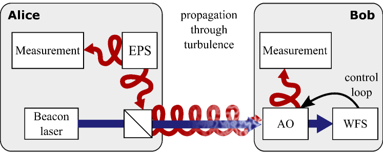
Let us start with the setup here considered, shown in Fig. 1. In Alice’s laboratory, a biphoton is generated in a maximally entangled (Bell) OAM qubit state, e.g.,

$$|\Phi_{0}\rangle=\frac{1}{\sqrt{2}}\left(|-l_{0},l_{0}\rangle+|l_{0},-l_{0}\rangle\right)\,,$$ (1)

where $|\pm l_{0}\rangle$ denotes a single photon state of a Laguerre-Gauss (LG) mode $LG_{0,\pm l_{0}}({\bf r},0)$ Allen et al. (1992) with radial index 0 and azimuthal index $\pm l_{0}$, at $z=0$ (${\bf r}$ is the transverse coordinate). The constituent photons thus carry an OAM of either $+\hbar l_{0}$ or $-\hbar l_{0}$ Allen et al. (1992). We assume a typical scenario Krenn et al. (2015) in which one of the photons stays in Alice’s laboratory, while the other one is sent to Bob, via a free-space link of length $L$. The first photon remains in its initial state, in contrast to the second photon which experiences turbulence-induced distortions.

II.2 Evolution of quantum states

The evolution under these distortions, for a particular realization of density variations of the medium, can be described by a unitary operator $U_{turb}(L)$ Roux (2014), such that propagation of single photon states $|\pm l_{0}\rangle$ across a turbulent layer is given by $|\psi_{\pm l_{0}}\rangle=U_{turb}(L)|\pm l_{0}\rangle$. The photon at Alice’s disposal is not affected by turbulence and we thus act with the identity operator $\openone$ thereupon to obtain the biphoton output state

$$|\Phi\rangle=\{\openone\otimes U_{turb}(L)\}|\Phi_{0}\rangle,$$ (2a)

$$|\tilde{\Phi}\rangle=\{\openone\otimes U_{AO}U_{turb}(L)\}|\Phi_{0}\rangle,$$ (2b)

in the absence and in the presence of AO correction, respectively. In our simulation, we evaluate the unitary operator $U_{turb}(L)$ implicitly, by connecting the mode functions of the input and output states using the extended Huygens-Fresnel principle (see Appendix A).

Since we have no interest in the specific realizations of turbulence, we need to perform a disorder average of the output biphoton states over different realizations, to obtain the mixed state

$$\sigma =\Big{\langle}|\Phi\rangle\langle\Phi|\Big{\rangle},$$ (3)

where $\langle\cdots\rangle$ denotes the disorder average. Finally, Bob’s photon is projected onto the encoding subspace, while Alice’s photon already is in this subspace. We describe this procedure by the operator $\openone\otimes\Pi_{0}$, where $\Pi_{0}=|-l_{0}\rangle\langle-l_{0}|+|l_{0}\rangle\langle l_{0}|$. The disorder averaged projected biphoton state thus reads

$$\rho=(\openone\otimes\Pi_{0})\sigma(\openone\otimes\Pi_{0})/\mathcal{N},$$ (4)

where the factor $\mathcal{N}={\rm tr}\{(\openone\otimes\Pi_{0})\sigma\}$ is required for renormalization. We recall that an average trace $\mathcal{N}<1$ of the density matrix indicates losses which may render quantum communication impossible.

In a final step, we have to evaluate the disorder averaged output state’s entanglement. This can be quantified via concurrence Wootters (1998)

$$C=\mathrm{max}\left\{\sqrt{\lambda_{1}}-\sqrt{\lambda_{2}}-\sqrt{\lambda_{3}}-\sqrt{\lambda_{4}},0\right\},$$ (5)

where the $\lambda_{i}$ are the eigenvalues, in decreasing order, of the matrix $\mathcal{R}=\rho(\sigma_{y}\otimes\sigma_{y})\rho^{*}(\sigma_{y}\otimes\sigma_{y})$, and $\sigma_{y}$ denotes the second Pauli matrix. When AO compensation is employed, we simply need to replace $|\Phi\rangle$ with $|\tilde{\Phi}\rangle$ in Eq. (3).

In the following, we present the details of the numerical simulation of the atmospheric channel and of the adaptive optics system.

II.3 Numerical simulation details

II.3.1 Multiple phase screen method

In our numerical simulations, we implemented the extended Huygens-Fresnel principle via a multiple phase screen approach. Therein, three-dimensional turbulence is described by equally spaced thin phase screens. Each screen introduces random phase distortions in accordance with Kolmogorov turbulence theory Andrews and Phillips (2005) and the beam experiences free diffraction in vacuum between the screens. The random phase screens were generated using the Kolmogorov spectral density $\Phi_{n}(\kappa)=0.033C_{n}^{2}\kappa^{-11/3}$, where $\kappa$ is the spatial wave vector in the transverse plane and $C_{n}^{2}$ is the turbulence phase structure constant Andrews and Phillips (2005); Schmidt (2010). Furthermore, the vacuum propagation between the phase screens was performed with a Fresnel propagator Bakx (2002), while the phase screens were obtained by the subharmonic method using seven subharmonic orders Lane et al. (1992).

For the final simulations, we chose four phase screens – to properly account for moderate scintillation, while we used a single screen for validation of our numerical procedure (see next section). The number of phase screens was determined by requiring for each partial propagation step to have a Rytov variance $\sigma_{R}^{2}<0.5$ for the chosen propagation distance of $L=500$ m and range of $C_{n}^{2}$ values. We simulated 19 values of the turbulence strength $C_{n}^{2}$ between $1.4\times 10^{-15}$m^-2/3 (weak turbulence) and $1.5\times 10^{-13}$m^-2/3 (moderate turbulence), while each data point was obtained from averaging over 1000 realizations of the turbulent phase screens. Given $C_{n}^{2}$, $L$, and $k=2\pi/\lambda$, one can obtain the transverse turbulence correlation length or Fried parameter $r_{0}=(0.423C_{n}^{2}k^{2}L)^{-3/5}$ Andrews and Phillips (2005) which fixes the turbulence strength $w_{0}/r_{0}$. In addition, we assume a telescope diameter of 0.2 m at Bob’s receiver which is a reasonable aperture size available both as a lens or mirror telescope Krenn et al. (2015). The large diameter ensures that most photons are received despite diffraction and turbulence-induced broadening and wandering of the light beam. Based on these simulation parameters, we calculate the biphoton output state in the $\pm l_{0}$ subspace from the overlap between the received field and the non-perturbed initial OAM modes. All calculations were carried out on a 0.4 m wide grid with $512\times 512$ points for a wavelength of 1064 nm and an initial beam waist of the OAM beams of $w_{0}=0.03$ m. Since the extent of the LG intensity profile increases as $\sqrt{l_{0}+1}$ with $l_{0}$ ($p=0$) Andrews and Phillips (2005), we chose a beam waist for the beacon to be $2.45\,w_{0}$. Thereby, we ensured an overlap with the intensity profiles of all simulated OAM modes (up to $l_{0}=5$).

II.3.2 Single-phase-screen validation

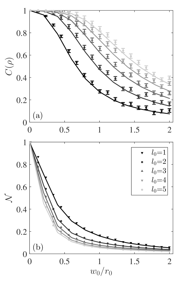
To validate our numerical routine, we first simulated the propagation with a single phase screen, in which case analytical results exist Leonhard et al. (2015) and agree with the earlier theoretical Smith and Raymer (2006) and experimental Hamadou Ibrahim et al. (2013) studies of concurrence decay in atmospheric turbulence. Figure 2 shows good agreement both for the concurrence (a) and the trace (b), where solid lines correspond to the analytical theory and points to our numerical data.

Figure 2: Validation of the simulation routine with a single phase screen, (a) concurrence and (b) trace of the final density matrix. Solid lines correspond to analytical results while points refer to numerical data. Error bars in (a) are obtained via error propagation from the standard deviation of the mean on the elements of $\rho$ (see Appendix B). In (b), the standard deviation of the mean is smaller than the size of the symbols.

II.4 Adaptive optics system

To measure and correct turbulence-induced distortions, we propose to use an AO system which consists of a beacon laser, a wavefront sensor and corrective elements such as deformable or tip/tilt mirrors. In state-of-the-art AO systems Tyson (2011), the time required to perform phase measurements and adjust the mirror into a new position is shorter than the typical timescale of atmospheric changes Milonni (1999), which allows us to neglect the dynamics of the atmosphere. The classical beacon beam (typically, a Gaussian laser beam Ren et al. (2014a)) is sent prior to and along the same path as the quantum light. Therefore, we can use its phase, $\varphi_{B}({\bf r})$, extracted via the wave-front sensor, to correct the phase distortion imprinted onto the single photons. Formally, we can express the action of AO by a unitary operator to find the corrected single photon state $|\tilde{\psi}_{\pm l_{0}}\rangle=U_{AO}U_{turb}(L)|\pm l_{0}\rangle$ at Bob’s receiver. The mode function associated with this corrected state is given by $\tilde{\psi}_{\pm l_{0}}({\bf r},L)=\exp\{-i\varphi_{B}({\bf r})\}\psi_{\pm l_{0}}({\bf r},L)$, where $\psi_{\pm l_{0}}({\bf r},L)$ is the mode function associated with the state $|\psi_{\pm l_{0}}\rangle$.

Figure 3: Concurrence $C$ (5), (a)-(c) and trace $\mathcal{N}$, (d)-(f), of the disorder averaged and projected biphoton output state $\rho$ plotted against the effective turbulence strength $w_{0}/r_{0}$, for different degrees of adaptive optics compensation: (a,d) without compensation, (b,e) ideal and (c,f) tip/tilt AO. Note the different scale of the $y$-axis in (b). Error bars in (a)-(c) are obtained via error propagation from the standard deviation of the mean on the elements of $\rho$ (see Appendix B). In (d)-(f) the standard deviation of the mean is smaller than the size of the symbols.

The evaluation of the phase $\varphi_{B}({\bf r})$, and hence of $U_{AO}$ in Eq. (2b), is based upon two ways of modeling the AO system. The first assumes an ideal system able to sense the phase $\varphi_{B,\infty}({\bf r})$ of the beacon field with arbitrary resolution, and to adapt the deformable mirror’s surface correspondingly. The second assumes the simplest AO possible which corrects only for a tilt of the wavefront, with respect to the receiver plane. In an experiment, this minimalistic scenario is achieved by a single flat mirror which can rotate along both axes perpendicular to the propagation direction – a so-called tip/tilt (TT) mirror. Our calculation of the required mirror rotation, similar to a typical experimental implementation, is based on the Fourier-transforming properties of an ideal lens. Accordingly, a tilted input field is transformed into a displaced focal spot. The center of mass of the focal plane intensity thus determines the rotation of the mirror, and thereby, $\varphi_{B,TT}({\bf r})$ Tyson (2011). These optimal and minimalistic AO scenarios allow us to establish an upper and a lower bound for the performance of a real AO system hereafter.

III Results

III.1 State’s entanglement and trace

With the above premises, we can now assess the potential of AO for state and entanglement transmission.

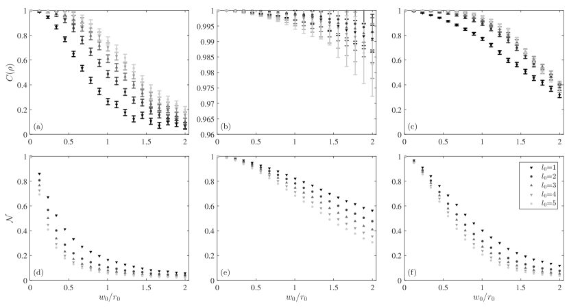
The top row of Fig. 3 displays our results for the entanglement evolution under turbulence, without (a) and with optimal (b) or minimalistic (c) AO compensation. Figure 3(a) establishes the well-known result that, the larger the initial OAM value $l_{0}$, the more robust entanglement is against (weak and moderate) turbulence Leonhard et al. (2015); Hamadou Ibrahim et al. (2013). Figure 3(b) shows that the ideal AO dramatically enhances the output state concurrence, to the extent of being almost fully preserved even in moderate turbulence. It might still be surprising that our idealized AO cannot completely recover the initial concurrence. To understand this, we need to consider that diffraction transforms phase distortions into intensity fluctuations, so-called scintillation Andrews and Phillips (2005). It then becomes clear that phase-only AO compensation cannot correct for such intensity distortions and is therefore most efficient for weak to moderate scintillation, i.e. for medium propagation distances and moderate turbulence strengths.

Furthermore, ideal correction inverts the trend observed in Fig. 3(a), providing slightly better stability to OAM modes with smaller $l_{0}$. As for tip/tilt correction, see Fig. 3(c), all curves but for $l_{0}=1$ collapse approximately onto one line for $w_{0}/r_{0}\gtrsim 1.5$. Both these observations from (b) and (c) suggest that AO is less effective for higher order OAM modes. We believe that this is due to the different beam geometries of the OAM modes and of the Gaussian mode beacon laser, respectively. The OAM modes have ring-like intensity patterns with vanishing intensity at the optical vortex – where the Gaussian beacon has its maximum intensity. Furthermore, OAM modes have a broader intensity profile which increases with $\sqrt{l_{0}+1}$ Paterson (2005) while the Gaussian beacon’s intensity is essentially localized within a fixed area leading to a decreasing overlap of beacon and OAM beam with increasing $l_{0}$. To reduce this effect, we have chosen a 2.45 times larger beam waist for the beacon than $w_{0}$ in all of our presented results to ensure an overlap with all modes up to $l_{0}=5$. A more quantitative analysis of these geometry-induced effects requires further optimization of the beacon parameters, and a more detailed adaptive optics system design which is beyond the scope of our present contribution.

Figure 4: Crosstalk-induced detection error contribution $R$, see Eq. (6), to the quantum bit error rate as a function of $w_{0}/r_{0}$, (a) without turbulence compensation, (b) with an ideal, and (c) with tip/tilt AO. Dashed horizontal lines in (a,c) indicate the security threshold of 11% Gisin et al. (2002) (note the different scale of the $y$-axis in (b)). Error bars represent the standard deviation of the mean.

The bottom row of Fig. 3 quantifies the loss of the trace ${\mathcal{N}}$ of the averaged output state’s density matrix as a consequence of the turbulence-induced crosstalk with OAM modes different from $\pm l_{0}$ Anguita et al. (2008). We find that both, ideal (e) and tip/tilt (f), AO lead to a noteworthy enhancement of the trace as compared to the uncompensated case (d). Consequently, the number of photons lost due to scattering outside the encoding subspace can be reduced, which increases the signal-to-noise ratio. For example, at $w_{0}/r_{0}=1$, tip/tilt compensation increases the trace by a factor between 2 and 4, and ideal AO even achieves factors between 5 and 13, depending on $l_{0}$. Interestingly, higher-order OAM modes exhibit a stronger relative trace enhancement as compared to lower-order modes, both for ideal and tip/tilt AO. Consequently, the number of detectable photons is increased also in higher-order OAM modes which are more sensitive to crosstalk. AO could thus enable studies of entanglement transmission in state spaces larger than those demonstrated to date.

Let us finally discuss why the efficiency of AO is different for the state’s entanglement as compared to its trace. As already mentioned, turbulence causes not only phase, but also intensity fluctuations, which cannot be compensated by AO. Residual intensity fluctuations lead to crosstalk and population of OAM modes inside and outside the encoding subspace, respectively, even in the case of ideal AO correction. The low residual crosstalk between the modes $\pm l_{0}$ results in a weak reduction of concurrence. In contrast, small populations in each of the modes outside the encoding subspace result in a relatively large cumulative effect on the trace of the final state. Additionally, the finite receiver aperture could enhance photon losses.

III.2 Qubit error rate

We finally address an application of our findings in the context of quantum cryptography, where the security of the communication channel is of particular importance. To judge whether an eavesdropper may have gained enough information to render communication insecure, Alice and Bob can evaluate the quantum bit error rate (QBER) on a subset of their measurements Gisin et al. (2002). In the case of entangled OAM states, intermodal crosstalk is a source of detection errors contributing to the QBER. Other, OAM-unrelated, effects, such as detector efficiency and noise statistics, can also contribute to the QBER of the communication channel Gisin et al. (2002). We here restrict our calculations to the detection error rate $R$ caused by crosstalk,

$$R=\frac{1}{\mathcal{N}}\Big{\langle}|\langle+l_{0}|U_{turb}|-l_{0}\rangle|^{2}+|\langle-l_{0}|U_{turb}|+l_{0}\rangle|^{2}\Big{\rangle}.$$ (6)

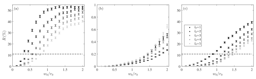
It is well-known Gisin et al. (2002) that the QBER and, thus, $R$ has to remain below 11% for secure communication.

Figure 4 shows the dependence of $R$ on the turbulence strength, in the absence of AO (a), for ideal AO (b), and for tip/tilt AO (c). Without AO, $R$ quickly prevents secure communication. With tip/tilt correction, the security threshold can be shifted to approximately two times larger turbulence strengths. A dramatic improvement is achieved by ideal AO, with $R<1\%$, such that secure communication can be achieved in the entire range of turbulence strengths considered here, provided all other contributions to QBER remain small enough.

IV Conclusion

In summary, we studied the efficiency of adaptive optics in preventing the loss of entanglement and of norm of OAM qubit states in atmospheric turbulence. Whereas without AO compensation both concurrence and trace rapidly decay with increasing turbulence strength, even minimalistic (tip/tilt) correction allows for an enhancement of the latter quantities by a factor of two to four. These results suggest that state of the art AO systems Petit et al. (2016), able to correct higher order aberrations of the wave front, bear the potential to enhance these factors still further – up to the almost complete restoration of entanglement and an increase of the trace by a factor between five and thirteen, in the ideal case.

While technically more involved in theory as well as in experiment, there is no fundamental obstacle to port the here described method to higher-dimensional OAM-entangled states. Furthermore, we believe that with higher-dimensional states we can push quantum communication protocols based on OAM states to longer propagation distances and worse turbulence condition, since the security threshold increases with increasing the dimensionality of the states Gisin et al. (2002). Likewise, our results imply that AO methods hold some promise to improve the fidelity of other quantum information protocols which suffer from mode distortions by uncontrolled errors Welte et al. (2017).

Appendix A Derivation of the output density matrix

We employ the extended Huygens-Fresnel principle Andrews and Phillips (2005); Ren et al. (2014a) to describe field propagation across a turbulent medium. According to this principle, the mode function of the output, single photon, state $|\psi_{\pm l_{0}}\rangle=U_{turb}(L)|\pm l_{0}\rangle$ is expressed by an integral,

$$\psi_{\pm l_{0}}({\bf r},L)=\int d^{2}r^{\prime}h({\bf r},{\bf r}^{\prime},L)LG_{0\pm l_{0}}({\bf r}^{\prime},0),$$ (7)

where $h({\bf r},{\bf r}^{\prime},L)=\langle{\bf r},L|U_{\text{turb}}(L)|{\bf r}^{\prime},0\rangle$ is the spatial response function which incorporates scattering-in-turbulence and diffraction effects.

On the other hand, the single photon state $|\psi_{\pm l_{0}}\rangle$ can be expanded in the OAM basis as,

$$|\psi_{\pm l_{0}}\rangle=\sum_{pl}g^{\pm l_{0}}_{pl}|pl\rangle,$$ (8)

where $|pl\rangle$ denotes a single photon state of an $LG_{pl}$ mode and the coefficients $g^{\pm l_{0}}_{pl}$ are given by the overlap integral,

$$g^{\pm l_{0}}_{pl}=\int d^{2}r\,\psi_{\pm l_{0}}({\bf r},L)LG^{*}_{pl}({\bf r},L).$$ (9)

In our numerical calculations, the integral in the above equation is replaced by a finite sum over the pixels in our calculation grid. The biphoton output state in Eq. (2a), postselected in the encoding subspace, can be expressed in the OAM basis as

$$(\openone\otimes\Pi_{0})|\Phi\rangle=\frac{1}{\sqrt{2}}(a|l_{0},l_{0}\rangle\!+\!b|\!-\!l_{0},l_{0}\rangle\!+\!c|l_{0},\!-l_{0}\rangle\!+\!d|\!-l_{0},\!-l_{0}\rangle),$$ (10)

where the expansion coefficients read

$$a :=\langle l_{0}|U_{turb}(L)|-l_{0}\rangle=g^{-l_{0}}_{0l_{0}}\,,$$ (11a)

$$b :=\langle l_{0}|U_{turb}(L)|l_{0}\rangle=g^{l_{0}}_{0l_{0}}\,,$$ (11b)

$$c :=\langle-l_{0}|U_{turb}(L)|-l_{0}\rangle=g^{-l_{0}}_{0-l_{0}}\,,$$ (11c)

$$d :=\langle-l_{0}|U_{turb}(L)|l_{0}\rangle=g^{l_{0}}_{0-l_{0}}\,.$$ (11d)

By definition, $b$ and $c$ are the survival amplitudes, whereas $a$ and $d$ – the crosstalk amplitudes Leonhard et al. (2015). In terms of these quantities, the average density matrix in Eq. (3) is given by

$$\rho =\frac{1}{\mathcal{N}}\begin{pmatrix}\langle|a|^{2}\rangle&\langle a^{*}b\rangle&\langle a^{*}c\rangle&\langle a^{*}d\rangle\\ \langle a^{*}b\rangle&\langle|b|^{2}\rangle&\langle b^{*}c\rangle&\langle b^{*}d\rangle\\ \langle c^{*}a\rangle&\langle c^{*}b\rangle&\langle|c|^{2}\rangle&\langle c^{*}d\rangle\\ \langle d^{*}a\rangle&\langle d^{*}b\rangle&\langle d^{*}c\rangle&\langle|d|^{2}\rangle\end{pmatrix},$$ (12)

with the normalization constant $\mathcal{N}=\langle|a|^{2}+|b|^{2}+|c|^{2}+|d|^{2}\rangle$. Using Eqs. (11a-d), we can also write the QBER in Eq. (6) as

$$R=\langle|a|^{2}+|d|^{2}\rangle/\mathcal{N}.$$ (13)

All previous expressions concerned wave propagation without the AO compensation, but they can easily be adapted to the case when AO correction of the phase front is present. Indeed, the mode function for the AO-compensated states $|\tilde{\psi}_{\pm l_{0}}\rangle$ is given by

$$\tilde{\psi}_{\pm l_{0}}({\bf r},L)=e^{-i\varphi_{B}({\bf r})}\psi_{\pm l_{0}}({\bf r},L),$$ (14)

where $\varphi_{B}({\bf r})$ is either $\varphi_{B,\infty}({\bf r})$ (ideal phase correction) or $\varphi_{B,TT}({\bf r})$ (tip/tilt correction). Furthermore, the AO-compensated state reads

$$|\tilde{\psi}_{\pm l_{0}}\rangle=\sum_{pl}\tilde{g}^{\pm l_{0}}_{pl}|pl\rangle,$$ (15)

with

$$\tilde{g}^{\pm l_{0}}_{pl}=\int d^{2}r\,\psi_{\pm l_{0}}({\bf r},L)LG^{*}_{pl}({\bf r},L)e^{-i\varphi_{B}({\bf r})}.$$ (16)

Analogously, when we expand the biphoton state $|\tilde{\Phi}\rangle$ [see Eq.  (2b)] in the OAM basis, we arrive at equations similar to Eqs. (10)-(13).

Appendix B Error on concurrence

Here we discuss the method to obtain the errors of concurrence through the propagation of the statistical errors of the output density matrix.

Our derivation below follows closely that in Ref. Ibrahim (2013), except that we used perturbation theory for non-Hermitian matrices (see below). First of all, we used the Bloch representation of the density matrix, which renders matrix elements (and consequently, errors) thereof real. In the Bloch representation, the density matrix reads

$$\rho=\sum_{i,j=0}^{3}B_{ij}\sigma_{i}\otimes\sigma_{j},$$ (17)

where $B_{ij}=\text{tr}(\rho\,\sigma_{i}\otimes\sigma_{j})$ are the Bloch coefficients, $\sigma_{0}$ is the $2\times 2$ identity matrix and $\sigma_{1,2,3}$ are the three Pauli matrices. Wootters’ concurrence is a function of the eigenvalues of the non-Hermitian matrix $\mathcal{R}$ given by

$$\mathcal{R}=\bar{\rho}(\sigma_{y}\otimes\sigma_{y})\bar{\rho}^{*}(\sigma_{y}\otimes\sigma_{y}),$$ (18)

which can be expressed in the Bloch representation as

$$\mathcal{R} =\sum_{ijkl=0}^{3}B_{ij}B_{kl}(\sigma_{i}\otimes\sigma_{j})(\sigma_{y}\otimes\sigma_{y})(\sigma_{k}\otimes\sigma_{l})^{*}(\sigma_{y}\otimes\sigma_{y}),$$

$$=\sum_{ijkl=0}^{3}B_{ij}B_{kl}\Gamma_{ijkl}.$$ (19)

where the four-index tensor $\Gamma_{ijkl}=(\sigma_{i}\sigma_{y}\sigma_{k}^{*}\sigma_{y})\otimes(\sigma_{j}\sigma_{y}\sigma_{l}^{*}\sigma_{y})$. We calculated the error on concurrence by propagating the error on the Bloch coefficients $\Delta B_{ij}$, which was calculated as standard deviation of the mean, assuming $B_{ij}$ to be statistically independent.

Using standard error propagation on Eq. (5), we expressed the error on concurrence as

$$\left(\Delta C\right)^{2}=\sum_{i=1}^{4}\left(\frac{\partial C}{\partial\lambda_{i}}\right)^{2}\left(\Delta\lambda_{i}\right)^{2}=\sum_{i=1}^{4}\left(\frac{1}{2}\frac{\Delta\lambda_{i}}{\sqrt{\lambda_{i}}}\right)^{2},$$ (20)

where $\Delta\lambda_{i}$ are the errors on the eigenvalues of the matrix $\mathcal{R}$. To calculate the errors $\Delta\lambda_{i}$, we first found the error on the matrix $\mathcal{R}$ as

$$\Delta\mathcal{R} =\sum_{mn=0}^{3}\frac{\partial R}{\partial B_{mn}}\Delta B_{mn},$$

$$=\sum_{klmn=0}^{3}(B_{kl}\Gamma_{mnkl}+B_{kl}\Gamma_{klmn})\Delta B_{mn}.$$ (21)

Finally, we used perturbation theory for non-Hermitian matrices James et al. (2001) to calculate the errors on the eigenvalues as

$$\Delta\lambda_{i}=W^{\dagger}_{i}\Delta\mathcal{R}V_{i},$$ (22)

where $W_{i}$ ($V_{i}$) are the left (right) eigenvectors of $\mathcal{R}$.

References

- Allen et al. (1992) L. Allen, M. W. Beijersbergen, R. J. C. Spreeuw, and J. P. Woerdman, Phys. Rev. A 45, 8185 (1992).
- Molina-Terriza et al. (2007) G. Molina-Terriza, J. P. Torres, and L. Torner, Nat. Phys. 3, 305 (2007).
- Krenn et al. (2014) M. Krenn, M. Huber, R. Fickler, R. Lapkiewicz, S. Ramelow, and A. Zeilinger, PNAS 111, 6243 (2014).
- Andrews and Babiker (2012) D. L. Andrews and M. Babiker, eds., The Angular Momentum of Light (Cambridge University Press, Cambridge, UK, 2012).
- Mirhosseini et al. (2015) M. Mirhosseini, O. S. Magaña-Loaiza, M. N. O’Sullivan, B. Rodenburg, M. Malik, M. P. J. Lavery, M. J. Padgett, D. J. Gauthier, and R. W. Boyd, New J. Phys. 17, 033033 (2015).
- Bechmann-Pasquinucci and Peres (2000) H. Bechmann-Pasquinucci and A. Peres, Phys. Rev. Lett. 85, 3313 (2000).
- Bourennane et al. (2001) M. Bourennane, A. Karlsson, and G. Björk, Phys. Rev. A 64, 012306 (2001).
- Paterson (2005) C. Paterson, Phys. Rev. Lett. 94, 153901 (2005).
- Krenn et al. (2016) M. Krenn, J. Handsteiner, M. Fink, R. Fickler, R. Ursin, M. Malik, and A. Zeilinger, PNAS 113, 13648 (2016).
- Vallone et al. (2014) G. Vallone, V. D’Ambrosio, A. Sponselli, S. Slussarenko, L. Marrucci, F. Sciarrino, and P. Villoresi, Phys. Rev. Lett. 113, 060503 (2014).
- Sit et al. (2017) A. Sit, F. Bouchard, R. Fickler, J. Gagnon-Bischoff, H. Larocque, K. Heshami, D. Elser, C. Peuntinger, K. Günthner, B. Heim, C. Marquardt, G. Leuchs, R. W. Boyd, and E. Karimi, Optica 4, 1006 (2017).
- Krenn et al. (2015) M. Krenn, J. Handsteiner, M. Fink, R. Fickler, and A. Zeilinger, PNAS 112, 14197 (2015).
- Rubinsztein-Dunlop et al. (2017) H. Rubinsztein-Dunlop, A. Forbes, M. V. Berry, M. R. Dennis, D. L. Andrews, M. Mansuripur, C. Denz, C. Alpmann, P. Banzer, T. Bauer, E. Karimi, L. Marrucci, M. Padgett, M. Ritsch-Marte, N. M. Litchinitser, N. P. Bigelow, C. Rosales-Guzmán, A. Belmonte, J. P. Torres, T. W. Neely, M. Baker, R. Gordon, A. B. Stilgoe, J. Romero, A. G. White, R. Fickler, A. E. Willner, G. Xie, B. McMorran, and A. M. Weiner, Journal of Optics 19, 013001 (2017).
- Milonni (1999) P. Milonni, Am. J. Phys. 67, 476 (1999).
- Tyson (2011) R. Tyson, Principles of Adaptive Optics, 3rd ed. (CRC Press, Boca Raton, 2011).
- Ren et al. (2014a) Y. Ren, G. Xie, H. Huang, C. Bao, Y. Yan, N. Ahmed, M. P. J. Lavery, B. I. Erkmen, S. Dolinar, M. Tur, M. A. Neifeld, M. J. Padgett, R. W. Boyd, J. H. Shapiro, and A. E. Willner, Optics Letters 39, 2845 (2014a).
- Ren et al. (2014b) Y. Ren, G. Xie, H. Huang, N. Ahmed, Y. Yan, L. Li, C. Bao, M. P. J. Lavery, M. Tur, M. A. Neifeld, R. W. Boyd, J. H. Shapiro, and A. E. Willner, Optica 1, 376 (2014b).
- Rodenburg et al. (2014) B. Rodenburg, M. Mirhosseini, M. Malik, O. S. Magaña-Loaiza, M. Yanakas, L. Maher, N. K. Steinhoff, G. A. Tyler, and R. W. Boyd, New J. Phys. 16, 033020 (2014).
- Li et al. (2014) M. Li, M. Cvijetic, Y. Takashima, and Z. Yu, Opt. Express 22, 31337 (2014).
- Smith and Raymer (2006) B. J. Smith and M. G. Raymer, Phys. Rev. A 74, 062104 (2006).
- Gopaul and Andrews (2007) C. Gopaul and R. Andrews, New J. Phys. 9, 94 (2007).
- Pors et al. (2011) B.-J. Pors, C. H. Monken, E. R. Eliel, and J. P. Woerdman, Opt. Express 19, 6671 (2011).
- Hamadou Ibrahim et al. (2013) A. Hamadou Ibrahim, F. S. Roux, M. McLaren, T. Konrad, and A. Forbes, Phys. Rev. A 88, 012312 (2013).
- Leonhard et al. (2015) N. D. Leonhard, V. N. Shatokhin, and A. Buchleitner, Phys. Rev. A 91, 012345 (2015).
- Roux et al. (2015) F. S. Roux, T. Wellens, and V. N. Shatokhin, Phys. Rev. A 92, 012326 (2015).
- Roux (2014) F. S. Roux, J. Phys. A: Math. Theor. 47, 195302 (2014).
- Wootters (1998) W. K. Wootters, Phys. Rev. Lett. 80, 2245 (1998).
- Andrews and Phillips (2005) L. C. Andrews and R. L. Phillips, Laser Beam Propagation through Random Media, Second ed. (SPIE Press, Bellingham, 2005).
- Schmidt (2010) J. D. Schmidt, Numerical Simulation of Optical Wave Propagation with examples in MATLAB (SPIE Press, Bellingham, Washington 98227-0010 USA, 2010).
- Bakx (2002) J. L. Bakx, Appl. Opt. 41, 4897 (2002).
- Lane et al. (1992) R. G. Lane, A. Glindemann, and J. C. Dainty, Waves Rand. Media 2, 209 (1992).
- Magnitskiy et al. (2015) S. Magnitskiy, D. Frolovtsev, V. Firsov, P. Gostev, I. Protsenko, and M. Saygin, J. Russian Laser Res. 36, 618 (2015).
- Gisin et al. (2002) N. Gisin, G. Ribordy, W. Tittel, and H. Zbinden, Rev. Mod. Phys. 74, 145 (2002).
- Anguita et al. (2008) J. A. Anguita, M. A. Neifeld, and B. V. Vasic, Appl. Opt. 47, 2414 (2008).
- Petit et al. (2016) C. Petit, N. Védrenne, M. Velluet, V. Michau, G. Artaud, E. Samain, and M. Toyoshima, Opt. Eng. 55, 111611 (2016).
- Welte et al. (2017) S. Welte, B. Hacker, S. Daiss, S. Ritter, and G. Rempe, Phys. Rev. Lett. 118, 210503 (2017).
- Ibrahim (2013) A. H. Ibrahim, The evolution of orbital-angular-momentum entanglement of photons in turbulent air, Ph.D. thesis, School of Chemistry and Physics, University of KwaZulu-Natal, Durban (2013).
- James et al. (2001) D. F. V. James, P. G. Kwiat, W. J. Munro, and A. G. White, Phys. Rev. A 64, 052312 (2001).