The model of an anomaly detector for HiLumi LHC magnets based on Recurrent Neural Networks and adaptive quantization

Abstract

This paper focuses on an examination of an applicability of Recurrent Neural Network models for detecting anomalous behavior of the CERN superconducting magnets. In order to conduct the experiments, the authors designed and implemented an adaptive signal quantization algorithm and a custom GRU-based detector and developed a method for the detector parameters selection.

Three different datasets were used for testing the detector. Two artificially generated datasets were used to assess the raw performance of the system whereas the 231 MB dataset composed of the signals acquired from HiLumi magnets was intended for real-life experiments and model training. Several different setups of the developed anomaly detection system were evaluated and compared with state-of-the-art OC-SVM reference model operating on the same data. The OC-SVM model was equipped with a rich set of feature extractors accounting for a range of the input signal properties.

It was determined in the course of the experiments that the detector, along with its supporting design methodology, reaches F1 equal or very close to 1 for almost all test sets. Due to the profile of the data, the $\mathtt{best\_length}$ setup of the detector turned out to perform the best among all five tested configuration schemes of the detection system. The quantization parameters have the biggest impact on the overall performance of the detector with the best values of input/output grid equal to 16 and 8, respectively. The proposed solution of the detection significantly outperformed OC-SVM-based detector in most of the cases, with much more stable performance across all the datasets.

1 Introduction

Table 1: Comparison of main parameters of LHC [1], HL-LHC [2] and FCC-hh [3].

	Perimeter	Particle energy	Luminosity	Integrated luminosity	Number of bunches
	[$\mathrm{km}$]	[$\mathrm{TeV}$]	[${10}^{34}\text{\,}{\mathrm{cm}}^{-2}\text{\,}{\mathrm{s}}^{-2}$]	[${\mathrm{fb}}^{-1}\text{\,}{\mathrm{d}}^{-1}$]
LHC	$27$	$7$	$1.0$	$0.47$	$2808$
HL-LHC	$27$	$7$	$5.0$	$2.8$†	$2748$
FCC-hh	$100$	$50$	$5.0$	$2.2$	$10\,600$

The LHC (Large Hadron Collider) was built with more than 20 years lasted effort of CERN (the European Organization for Nuclear Research) personnel and whole worldwide High Energy Physics community. The LHC consists of a $27\text{\,}\mathrm{km}$ ring located $100\text{\,}\mathrm{m}$ underground and filled mainly with superconducting magnets. The LHC started operating in 2008, and since that time it contributed to some pronounced scientific discoveries concerning Standard Model [4, 5].

Many research and development programs are continuously carried out to deliver improvements to the construction of numerous subsystems of the LHC. Currently, the most critical project, which already entered a construction phase, is the HL-LHC (High Luminosity LHC). This major upgrade is planned to be introduced between years 2023 and 2025. The primary goal is to increase the luminosity (rate of collisions) by a factor of five beyond its original design value, and the integrated (over a whole year) luminosity by a factor of ten [2]. It will be possible thanks to the development of several innovative technologies, mainly in the field of superconductivity.

Looking far into the future, the CERN started a study for next generation circular accelerator called FCC (Future Circular Collider) [3]. Preliminary assumptions concerning this project indicate that the FCC will be a ring with a circumference around four times longer than the tunnel currently used by LHC (Tab. 1). In such a vast project the importance of an intelligent automation will be much higher and may even be the only chance to maintain and operate the accelerator.

The modifications in the accelerator structure related to the HL-LHC project require, in turn, a creation of new solutions for the MPS (Machine Protection System), the LHC components maintenance and monitoring system, which is the responsibility of CERN TE-MPE (Technology Department - Machine Protection and Electrical Integrity) group. The main interest of the TE-MPE group is to maximise the availability of the machine while the high safety level is guaranteed.

A complexity of this task stems from an abundance of signals acquired from various LHC magnets and the real-time operation requirement. The system needs to process all the data and detect anomalies in such a time that will allow various automatic fault prevention procedures to run. Conventional anomaly detection systems, such as presented in section 3, cannot be used in this particular application due to a vast quantity of signals, very few anomaly cases and the hardware implementation in embedded systems requirement.

The primary goal of this study is a creation and verification of a model that can be used in the future design of a software and ultimately a hardware solution for an anomaly detection device suitable for application in particle accelerators. One of the promising research directions involves using NN (Neural Network) and ML (Machine Learning) algorithms for magnets monitoring, as well as anomaly detection. A real-time execution of ML algorithms requires dedicated, low latency architectures, such as FPGA (Field-Programmable Gate Array) or a digital ASIC (Application-Specific Integrated Circuit), which is an authors’ long-term research goal. The current work, presented in this paper, focuses on the development and verification of a dedicated solution involving adaptive quantization and RNN (Recurrent Neural Network). The created solution achieved very encouraging results for LHC magnets signals.

The presented research main contributions are as follows:

• development of an architecture for anomaly detection based on GRU (Gated Recurrent Unit),

• introduction of a new approach based on adaptive grid quantization,

• detector design procedure which accounts for the detector operation environment,

• development of a system level model suited for doing experiments with the adaptive grid-based approach; the software is available online [6].

The developed design procedure should allow reusing the researched solution for various use cases, requiring only a setup configuration changes.

The rest of the paper is organized as follows. Sections 2 and 3 provide background information about LHC and anomaly detection state of the art (including Recurrent Neural Networks usage), respectively. The quantization algorithm, the system description, and the developed methodology are explained in sections 4, 5, and 6. Next, the results of the experiments and their comparison to an alternative approach based on OC-SVM (One Class Support Vector Machine) method are presented in section 7. General discussion can be found in section 8. Finally, the conclusions of our research are presented in section 9 and the future work plans in section 10. Software variables used throughout the whole text are briefly summarized in A.

2 The Large Hadron Collider

2.1 Superconducting magnets

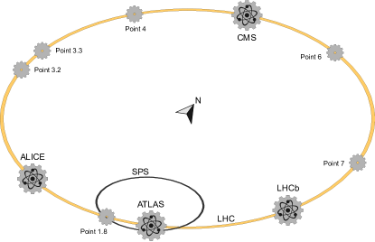
Figure 1: Diagram of the LHC and the related experiments (adapted from [7], © 2014-2017 CERN, license: CC-BY-3.0).

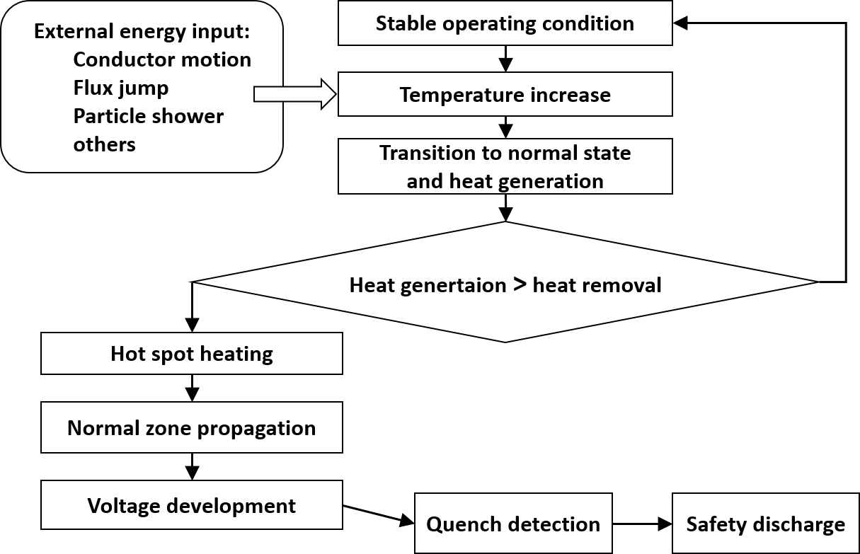
Figure 2: Flowchart describes what typically happens in case of an energy dissipation inside superconducting component (adapted from [8], © 2014-2017 CERN, license: CC-BY-4.0).

Table 2: Nominal conditions in the main dipole circuits of the LHC at the beginning and at the end of ramping up [1].

Parameter	Injection	Collision
Proton energy [$\mathrm{TeV}$]	$0.450$	$7$
Magnetic field [$\mathrm{T}$]	$0.535$	$8.33$
Supply current [$\mathrm{A}$]	$763$	$11\,850$
Energy stored [$\mathrm{MJ}$]	$4.483$	$1081.253$

The LHC, the largest and most powerful accelerator in the world, is divided into eight sectors (octants) (Fig. 1). The tunnel itself contains strings of superconducting magnets, accelerating cavities and many other necessary instruments. Two vacuum beam pipes are going through central part of an iron yoke of magnets.

The particles are produced and initially accelerated by the chain of smaller accelerators. Then, particles are delivered into the LHC with energy at injection level (see Tab. 2). During every turn around the whole trajectory, the energy of particle raises and synchronously the magnetic file produced by bending magnets must also be increased. This ramping process takes some time before the machine achieves a condition in which collisions are initiated. In this state, every $25\text{\,}\mathrm{ns}$ two particle clouds (bunches) collide in four interaction points denoted in the Fig. 1 by the names of experiments: ATLAS (A Toroidal LHC ApparatuS), CMS (Compact Muon Solenoid), ALICE (A Large Ion Collider Experiment), and LHCb (Large Hadron Collider beauty experiment). Products from each collision are observed by dedicated systems of particle detectors.

The primary goal of whole engineering effort at the LHC is to maintain the collision state of the accelerator as long as possible to give a chance to maximize the number of observed events. However, the quality of beams is decreasing with each collision, and, at some point, they stop being useful for physics experiments. At this stage of operation, the beams are dumped, the machine must ramp down and be filled with particles again. This whole work cycle can be interrupted at any time by a malfunction of one of the thousands of elements of the accelerator.

Table 3: General overview of the circuits powering the superconducting magnets of the LHC [9, 10]. The number of quenches as reported on 10 October 2016.

LHC Circuit	No of circuits	No of magnets in one circuit	No of quenches
RB	$8$	$154$	$1270$
RQ	$16$	$47$	$64$
IT	$8$	$4$	$18$
IPQ	$78$	$2$	$323$
IPD	$16$	$1$	$53$
$600\text{\,}\mathrm{A}$ EE	$202$	$m$	$425$
$600\text{\,}\mathrm{A}$ EEc	$136$	$1$ or $2$
$600\text{\,}\mathrm{A}$	$72$	$1$
$$80$\div$120\text{\,}\mathrm{A}$$	$284$	$1$	$116$
$60\text{\,}\mathrm{A}$	$752$	$1$	$44$

There are $1232$ dipole and $392$ quadrupole magnets that are crucial elements of the LHC (see Tab. 3 for the approximate list). The coils of those electromagnets are wound up with multi-filament cables. The filaments are made with niobium-titanium $\mathrm{Nb-Ti}$ alloy, with a copper matrix surrounding them. This kind of coils produces a magnetic field of $8\text{\,}\mathrm{T}$, sufficient to drive particles along the ring at $7\text{\,}\mathrm{TeV}$ energy. The coil conducts a high superconducting current, but sometimes, locally, in a random and uncontrolled way, it becomes normally-conducting. This event (a quench) is hazardous because it is connected with burst dissipation of energy stored in the superconducting circuit. It is not a malfunction, but a physical phenomenon which takes place in any superconducting circuit which does not meet a condition of cryogenic stability [11]. The superconducting magnets applied in the accelerators are designed as not safe in that sense. Many other design constraints make this an only feasible possibility. Therefore the QPS (Quench Protection System) was created at the LHC [12, 13].

QPS is a sophisticated subsystem dedicated to magnet coils monitoring and anomaly detection, supervising working condition changes during various phases of the system operation. The voltages on coils, busbars and current leads are acquired and stored in a database. The malfunctions or quenches are detected on-line when a value of the voltage exceeds a safety threshold. When this state lasts longer than a discrimination time, a trigger signal is generated to stop the operation of the whole accelerator and to discharge the energy stored in its circuits safely. The diagram presented in Fig. 2 summarizes the described scenario. Any undetected quench (false negative) can lead to catastrophic damages due to huge energy stored in magnetic field (Tab. 2). This energy must be discharged in a controlled manner.

For the High Luminosity upgrade of the LHC (HL-LHC) a new generation of niobium-tin $\mathrm{Nb_{3}Sn}$ superconducting magnets will be installed as the inner triplets quadrupoles (low beta quadrupoles MQXFA/B) and the $11\text{\,}\mathrm{T}$ dipoles (MBH) [14]. In particular, the inner triplets of the points 1 and 5, ATLAS and CMS, will be replaced while the $11\text{\,}\mathrm{T}$ dipoles will take the place of the standard LHC main dipoles on both the sides of point 7. The new magnets will be fed by a superconducting link with niobium-boron $\mathrm{MgB_{2}}$ cables [15].

The technologies used for reaching high magnetic field also implicate the development of a new protection system, and in particular of a dedicated detection system [16]. In fact, this kind of coils suffers from not only a quench but also from the so-called flux jumps [17], affecting the nature of voltage waveforms describing the state of superconducting magnets. In the ongoing magnet tests, the occurrences of these with the relate voltage spikes at a low current rate ($I<$4\text{\,}\mathrm{kA}$$) could represent an issue for the classical detection parameters (voltage threshold of $\pm$100\text{\,}\mathrm{mV}$$ and the evaluation time of $10\text{\,}\mathrm{ms}$). As a consequence, the strategy for the quench detection should be replaced with a new one based on dynamically set detection parameters [16].

2.2 Source of data for this study

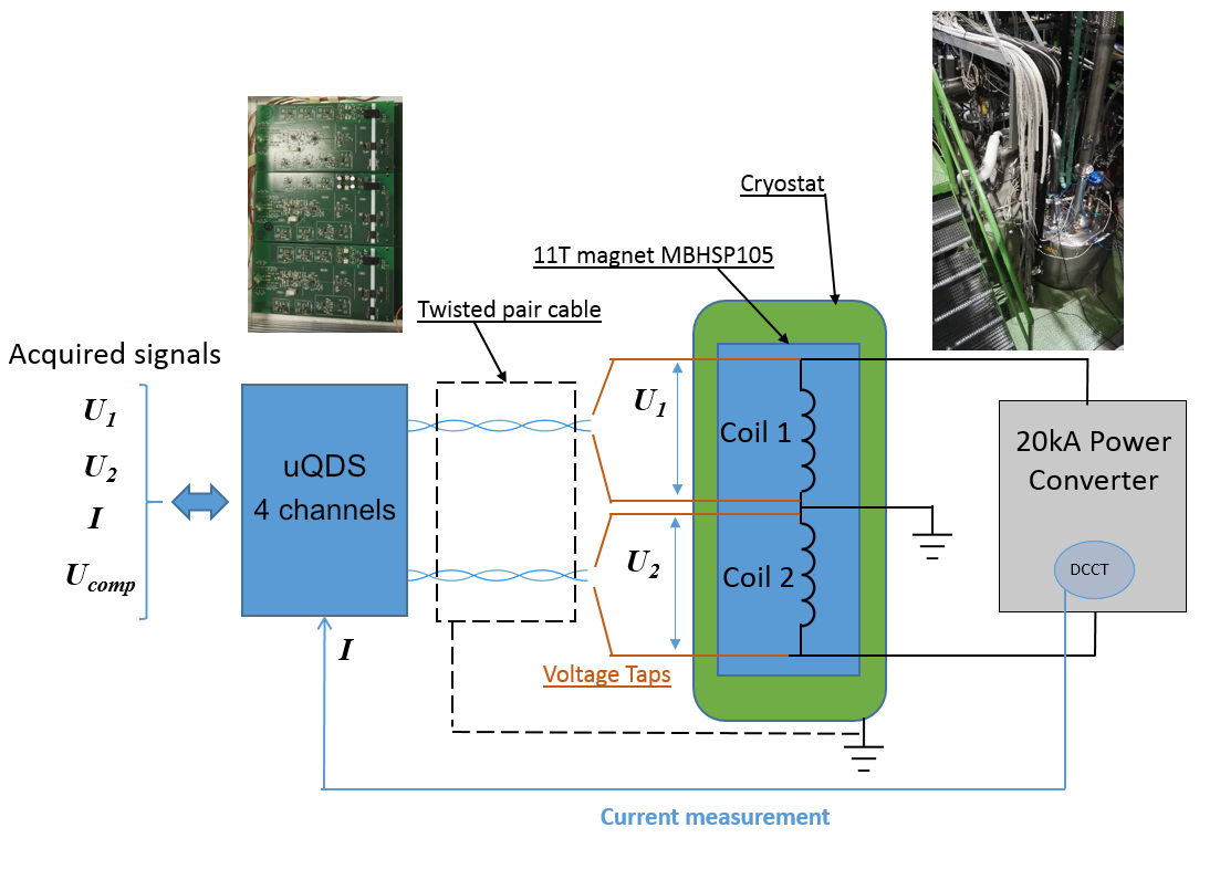
Figure 3: Measurement setup for the $11\text{\,}\mathrm{T}$ MBHSP105 magnet tests.

Any superconducting circuit which does not meet a condition of cryogenic stability needs permanent monitoring (logging) during testing, commissioning, and operation. In case of any event (e.g., quench) in a superconducting circuit a data with higher time resolution is also acquired and stored for analysis. Therefore, two dedicated database services were built at CERN. The logging data is stored in CALS (CERN Accelerators Logging Service), whereas the data acquired during an event is kept in a separate system named PM System (Post Mortem System).

The data used in this study is of the logging type. It was acquired during testing a new type of magnet designed for the HL-LHC project. The test was conducted at the Superconducting Magnet Test Facility (SM18) in November 2016. The test was performed on single aperture dipole magnet dedicated to delivering magnetic filed on the level of $11\text{\,}\mathrm{T}$. Therefore the coils of this magnet were wound with a cable made of niobium-tin $\mathrm{Nb_{3}Sn}$ superconducting material. The exact designation of the magnet is MBHSP105 [14].

The goal of the test was to train the magnet. A magnet training is an iterative procedure of magnet powering. At first, during ramping up a current, a magnet loses superconducting state (quench) long before reaching the expected critical current. During the next attempt, the current that could be reached before quench is higher. The process continues over all the next attempts, and the maximum current that could be reached increases quench after quench, slowly approaching a plateau.

In our case, the plateau was reached after several runs. Each run begun with ramping of magnet current with rate $50\text{\,}\mathrm{A}\text{/}\mathrm{s}$. After reaching the level of $8\text{\,}\mathrm{kA}$, the rate was lowered to the value of $10\text{\,}\mathrm{A}\text{/}\mathrm{s}$. The ramping with this rate was maintained up to a quench.

During the runs, the current and voltages in the coils of the magnet were measured using a device named uQDS (universal Quench Protection System) (ver. 1.0) [16]. The measurement setup is shown in the Fig. 3. The device was built with an analog to digital converter ADC (Analogue to Digital Converter) of the SAR (Successive Approximation Register) type with $20\text{\,}\mathrm{bit}$ resolution. The digital control of the acquisition was built with FPGA circuit of the IGLOO^®2 type from Microsemi^®. The sampling rate was $9.3\text{\,}\mathrm{kSPS}$ (sampling period $107.5\text{\,}\mathrm{\SIUnitSymbolMicro s}$).

The data of PM (Post Mortem) kind was also acquired during this training with a sampling rate of $100\text{\,}\mathrm{kSPS}$ but it was not used in this study.

3 State of the art

3.1 Overview

Monitoring time series signals changes is critical in many areas of engineering and real-life applications. It is mostly because roughly $80\text{\,}\mathrm{\char 37\relax}$ of the signals which occur in the world are temporal in their nature. Consequently, anomaly detection was heavily explored as a field over the last several decades and many methods were developed to address this challenging task [18, 19, 20]. It is worth noting that most of the anomaly detection tasks deal with quite asymmetric datasets which means that there are far few cases of anomalous behavior than regular ones. Furthermore, labeling the data is challenging task. Characteristics mentioned above lead to the preference of unsupervised methods over supervised ones when it comes to real-life applications. An ideal anomaly detection system should:

• be able to detect anomalies with the highest possible accuracy,

• be trained in unsupervised fashion,

• trigger no false alarms,

• work with data in a real-time,

• be completely adaptable (no hyper-parameters tuning).

Unfortunately, it is difficult to construct such a system not only because of a challenge to meet all of the requirements at the same time but also for the sake of a data profile. For instance, how frequently a model should be updated to account for seasonality of changes in the data is not always clear. Furthermore, real-time performance is not always at the premium. However, due to the rise of data volume and an increasing demand for speed at which the system should deliver results, we may expect the growing demand for real-time performance.

Anomaly detection systems in real-life applications are not ideal which means that they do not meet all the requirements enumerated on the list. They do not have to, as very often it is enough that a system detects most of the anomalies in a reasonably short time. Sometimes, however, for the sake of a task profile, it is critical that a system does not generate false alarms, even at the expense of a slightly lower overall accuracy. In some other cases, response accuracy is not as important as a low response time of the system. It can be observed while analyzing how anomaly detection systems developed over the past few decades [20] that there is a trade-off between response accuracy and reaction time. Consequently, depending on an expected performance three different groups of anomaly detection systems may be distinguished:

• offline,

• partially online,

• online.

The first category of the systems operates in an offline fashion which means that they are trained offline and work offline. Such solutions are well suited for processing large volumes of data at relatively low pace and usually require access to the whole dataset. Examples of such systems used in industrial applications are EGADS (Extendible Generic Anomaly Detection System) developed by Yahoo [21] and RPCA (Robust Principle Component Analysis) [22]. The EGADS is based on the assumption that integration of several methods within a single framework helps to address different kinds of anomalies. Such an approach is very sound in principle but comes at the cost of processing time which results from a necessity of weighting and incorporating contributions of different methods. There are also other solutions which can be classified into a category of offline systems [23, 24].

The second category of the algorithms is trained offline and work online. Complex and large models usually need to be trained offline because of the time it takes to complete the process. However, sometimes the model is small enough to be trained online, but it is still beneficial to conduct the training process offline as a result of an application profile and the system requirements.

In some applications, a system should be more sensitive to seasonal changes, and it is essential to train a model only during specific periods of time. There is a whole branch of clustering-based algorithms which are trained offline to subsequently work online [25, 26, 27, 28, 29, 30, 31, 32]. Time series are clustered according to their properties, and all the outliers which do not belong to one of the clusters are considered anomalies. An amount of clusters and the classification threshold are two of the more critical parameters which are to be chosen for the applications of those algorithms.

One of the standard solutions which fall in the second category is an approach based on OC-SVM. Several implementations of anomaly detection systems based on OC-SVM were proposed, and promising results were reported [33, 34, 35, 36, 37, 38, 39]. The methods based on RNNs, described in 3.2, also belong to that category.

The third kind of the anomaly detection systems adapts online which means that all the novelties which are detected are incorporated in the model [40, 41]. Next time the same phenomenon occurs in the input signal to the system, it will not be considered as an anomaly. In such an approach, the system continually adapts to the changing environment which may be beneficial in many scenarios. However, there are applications in which due to the seasonality it is recommended to update a model in well-defined moments of time.

There exist more advanced streaming anomaly detection methods, such as ESD, ARIMA (Autoregressive Integrated Moving Average), and Holt-Winters [42, 43, 44, 45], which are used in many industrial applications. A broad analysis of the modern anomaly detection systems is beyond the scope of this paper, for more in-depth review please see [19, 18, 20]. It is worth emphasizing that the area of novelty detection is expanding very fast which is driven by an exponential growth of available information and rising need for knowledge extraction. We may expect this trend to intensify as a result of an introduction of new hardware platforms which are capable of processing data faster [46, 47, 48].

3.2 Recurrent Neural Networks

The RNNs fundamentally differ from the FNNs (Feed-forward Neural Networks). The recurrent neural models learn to recognize patterns in the time domain. Consequently, they are capable of modeling signals in which patterns span over many time steps.

For many years, factors limiting the development and engineering applicability of recurrent neural networks existed. Those restrictions were associated with the possibility of learning very long patterns, with sequences length in tens or hundreds. Classical RNNs were not able to learn them due to the so-called vanishing (or exploding) gradient phenomenon. Scientists working in an RNN domain were aware of it occurring, not only in RNNs but also in deep FNNs. Therefore, extensive research was conducted, and in 1997 it resulted in development of the LSTM (Long Short-Term Memory) architecture by Jürgen Schmidhuber [49]. Unfortunately, due to the lack of computing power and limited available data quantities, LSTM-type networks were developing slowly. In the recent years, however, there was a considerable progress in RNNs. Many variants of the original LSTM algorithm were introduced, optimizing the original architecture. One of such a modifications is GRU [50, 51]. Short presentation of GRU architecture can be found in  C.

RNN networks were employed for anomaly detection task in different operational setups [52, 53, 54, 55, 56, 57]. The authors of [52] proposed an architecture of LSTM-based anomaly detector which incorporates both hierarchical approach and multi-step analysis. The proposed model capitalizes on a property of generalization which results from stacking of several RNN layers. The system in [52] was trained on regular data and verified on data containing anomalies. The authors used Gaussian distribution of an error signal - the difference between predicted and real values. Consequently, the module predicts several time steps into the future and fits the estimated error into the Gaussian distribution. Four different datasets were used to demonstrate the performance of the proposed solution.

There is a whole branch of LSTM-based anomaly detectors which exploit a property of inconsistent signal reconstruction in the presence of anomalies [55, 56]. The authors trained the model of the autoencoder on regular data and set a threshold above which the reconstruction error is considered an anomaly. The papers deal with acoustic signals, but such an approach may be efficiently employed in other domain such as videos [57]. Systems based on those principles may be trained in an end-to-end fashion. The presented models [55, 56] were trained on the publicly available datasets, and the results are superior in comparison with the other solutions.

4 Quantization algorithm

4.1 Previous work

Table 4: Notation used in quantizaton equations (1) - (7).

$n$	number of samples
$m$	number of classes (categories, bins); $m\in\mathbb{N}_{>0}$
$S_{\mathit{in}}$	signal input space
$S_{\mathit{norm}}$	normalized input space
$S_{\mathit{qs}}$	signal space after static quantization
$S_{\mathit{qa}}$	signal space after adaptive quantization
$\mathbf{edges}_{i}$	$i$-th quantization edge, see (7)
$\mathbf{sorted\_samples}_{i}$	$i$-th sample in the ascending sorted array of all available signal samples

Table 5: Percentage of samples per single class in training set.

			$\mathrm{\char 37\relax}$ of total samples per class
	no of classes	median bin width	minimum	maximum
static grid	$8$	$0.125$	$0\text{\,}\mathrm{\char 37\relax}$	$\sim 100\text{\,}\mathrm{\char 37\relax}$
	$16$	$0.0625$	$0\text{\,}\mathrm{\char 37\relax}$	$\sim 100\text{\,}\mathrm{\char 37\relax}$
	$100$	$0.01$	$0\text{\,}\mathrm{\char 37\relax}$	$\sim 81\text{\,}\mathrm{\char 37\relax}$
adaptive grid	$8$	$0.000\,35$	$\sim 8\text{\,}\mathrm{\char 37\relax}$	$\sim 14\text{\,}\mathrm{\char 37\relax}$
	$16$	$0.000\,18$	$\sim 2\text{\,}\mathrm{\char 37\relax}$	$\sim 7\text{\,}\mathrm{\char 37\relax}$
	$100$	$0.000\,03$	$\sim 0\text{\,}\mathrm{\char 37\relax}$	$\sim 1\text{\,}\mathrm{\char 37\relax}$

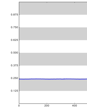
(a) Static grid

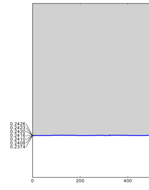
(b) Adaptive grid

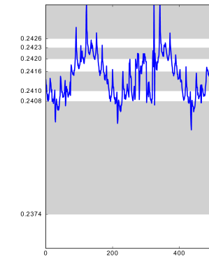
(c) Zoom of adaptive grid

Figure 4: Static (4(a)) vs. adaptive (4(b), 4(c)) quantization; $m=8$.

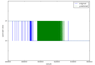
(a) Static quantization; $m=100$

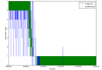
(b) Adaptive quantization; $m=8$

Figure 5: Models reacting to vertical shift in signal (same data fragment).

In the authors’ previous work concerning superconducting magnets monitoring [58] a RMSE (Root-Mean-Square Error) approach was used. It showed that RNNs are in fact able to model magnets behavior. However, it has several drawbacks that make it hard to use in practical anomaly detection applications.

Firstly, to adequately analyze anomalies using the RMSE it would be necessary to select a detection threshold. Such a threshold would be very arbitrary, since it is hard to discern what value, allowing to detect all anomalies, would be appropriate based on the results obtained from all the data, including regular operation.

Secondly, the resolution of such an anomaly detection would depend on used window size. Additionally, choosing too broad a window would result in anomaly potentially ’drowning’ in the correct data, while choosing too small could result in false positives. The window size would also influence the trained RNN accuracy.

Described drawbacks resulted in authors’ decision to switch from regression to a form of predictive classification. Initially, the signals were converted to classes using a static, evenly-spaced grid, mapping whole signal amplitude [59]. Both input signals and output one were mapped, and the model task was to predict output category given a tensor of input classes correctly. When the prediction and real signal did not match over a certain amount of samples, an anomaly was reported.

A static quantization process is mapping signal input space $S_{\mathit{in}}$ to $m$ classes (see Tab. 4 for notation used), that can potentially be represented by $\left\lceil\log_{2}m\right\rceil$ bits instead of initial $32$ or 64 per value. At first, as given by (1) - (2), the signal is normalized. Next, the normalized signal values are mapped to categories, using $m$ evenly-spaced bins spanning whole signal amplitude (3) - (4).

$$S_{\mathit{in}}:\mathbb{R}^{1\times n}\xRightarrow{\Pi_{\mathit{norm}}}S_{\mathit{norm}}:\left\{0\ldots 1\right\}^{1\times n},$$ (1)

$$\Pi_{\mathit{norm}}:\bigwedge_{x\in S_{\mathit{in}}}\bigvee_{y\in S_{\mathit{norm}}}~{}y=\frac{x-\min S_{\mathit{in}}}{\left|\max S_{\mathit{in}}-\min S_{\mathit{in}}\right|}.$$ (2)

$$S_{\mathit{norm}}\xRightarrow{\Pi_{\mathit{qs}}(m)}S_{\mathit{qs}}:\left\{0\ldots m-1\right\}^{1\times n},$$ (3)

$$\Pi_{\mathit{qs}}(m):\bigwedge_{x\in S_{\mathit{norm}}}\bigvee_{y\in S_{\mathit{qs}}}~{}y=\begin{cases}y\leqslant x\cdot m<y+1\text{~{}if~{}}x<1\\ y=m-1\text{~{}if~{}}x=1\end{cases}.$$ (4)

As a result of conducted experiments analysis, as well as formal static quantization algorithm scrutiny, the authors concluded that using evenly-spaced grid will not allow detecting anomalies effectively. It was due to the algorithm mapping most of the data to a minuscule number of categories, with the majority of them almost never being used (see Fig. 4(a) and Tab. 5). The end effect was that, on the one hand, it took a long time for a model to adapt to a vertical shift in data (Fig. 5(a)), resulting in false anomalies, and, on the other hand, smaller anomalies would have no chance to be detected. Additionally, since most of the categories were barely used, it resulted in wasting resources.

4.2 Adaptive grid

Analysis of previously mentioned experiments and algorithms resulted in a conclusion that a more advanced algorithm is needed. It should avoid the threshold-selection problem, allow to harvest the RNNs potential by using classification instead of regression and optimally use available resources. As a consequence, adaptive grid quantization algorithm was developed. Its principle of operation is mapping the input space to a fixed number of categories (bins) in such a way, that all categories have (ideally) the same samples cardinality as it is described by equations (5) - (7). As a result, bins widths are uneven, explicitly adjusted to the input signal (see Fig. 4(c) and Tab. 5). Each of the signals used in the model training has its own bins edges calculated. This approach allows to potentially maximize the utilization of the grid and minimize the consumption of resources.

$$S_{\mathit{norm}}\xRightarrow{\Pi_{\mathit{qa}}(m)}S_{\mathit{qa}}:\left\{0\ldots m-1\right\}^{1\times n},$$ (5)

$$\Pi_{\mathit{qa}}(m):\bigwedge_{x\in S_{\mathit{norm}}}\bigvee_{y\in S_{\mathit{qa}}}y=\begin{cases}\!\begin{multlined}\mathbf{edges}_{y}\leqslant x\cdot m<\mathbf{edges}_{y+1}\\[-10.0pt] \text{if~{}}x<1\end{multlined}\mathbf{edges}_{y}\leqslant x\cdot m<\mathbf{edges}_{y+1}\\[-10.0pt] \text{if~{}}x<1\\ y=m-1\text{~{}if~{}}x=1\end{cases},$$ (6)

$$\mathbf{edges}:\bigwedge_{0\leqslant y\leqslant m}\mathbf{edges}_{y}=\begin{cases}0\text{~{}if~{}}y=0\\ \!\begin{multlined}\mathbf{sorted\_samples}_{y\cdot\left\lceil\frac{n}{m}\right\rceil}\\[-10.0pt] \text{if~{}}0<y<m\end{multlined}\mathbf{sorted\_samples}_{y\cdot\left\lceil\frac{n}{m}\right\rceil}\\[-10.0pt] \text{if~{}}0<y<m\\ 1\text{~{}if~{}}y=m\end{cases}.$$ (7)

5 System description

5.1 Principle of operation

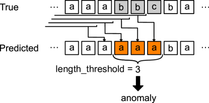
Figure 6: System principle of operation.

The detector principle of operation is a comparison between predicted and real signal values (Fig. 6). Whenever a new sample arrives, it can be used (in conjunction with previous samples) to predict the category of the next sample. Assuming that the model was trained to anticipate normal operating conditions ideally, any difference between the prediction and an actual arriving sample category means that an anomaly occurred.

In the practical applications, however, achieving the model perfection is not feasible: the data used to train the model, as well as real samples that the predictions will be compared with, contains noise. Given large enough pool of samples to learn from, the model should start to predict nearly ideal normal operation values, but even the actual normal operation samples will differ from that ideal due to noise. When an anomaly occurs, those differences should be much more pronounced. As a result, a method to discriminate between ’noise anomalies’ and actual anomalies is needed.

The simplest discriminating method is to check an anomaly candidate length. In previous work [59], authors assumed that a gap between available history data and prediction ($\mathtt{look\_ahead}$) must be bigger than $\mathtt{length\_threshold}$, so that, in case of an anomaly occurring, the model prediction would not get distorted by an irregular input. The size of this gap, in turn, further affected the model accuracy. However, after further research on the RNN behavior, the authors concluded that this condition is unnecessary since the model should (up to some point) ignore the anomalous sample in favor of available normal operation historical data, with this ’smoothing’ capability increasing with $\mathtt{look\_back}$ (history window) length. Predicting only one step forward ($\mathtt{look\_ahead}=1$) has an additional advantage of potentially decreasing system reaction time, especially in conjunction with more advanced anomaly discrimination methods.

5.2 Setup overview

Figure 7: Setup life cycle conceptual overview.

Figure 8: Example model generated for $\mathtt{out\_grid}$=8, $\mathtt{cells}$=64, $\mathtt{look\_back}$=16.

The system is coded in Python, using Keras [60] library with Theano [61] backend for the classifier implementation. The detector module consists of two main sub-modules, model and analyzer, and a few helper scripts. The conceptual overview of the single detector setup is presented in Fig. 7.

The system is prepared to work with normalized data, which are prepared and saved beforehand. Normalization process takes into account all available data, both from training and testing sets. All the data fed into the system at a later time would need to be prepared using the same scale, with out-of-range values clipped to $0.0$ or $1.0$ as relevant. All setup variants use the same normalized data.

Depending on the configuration, a particular system setup variant is created. The configuration includes options of data pre-processing (e.g., number of input/output categories or the bins edges calculation algorithm), the model hyper-parameters (such as an amount of layers, number of cells per layer, and batch size) and the analyzer rules (like minimum anomaly length or cumulative amplitude). Most of the configuration options are specified as arrays, allowing to test several setups and compare them easily. Models trained during each of the setups are automatically saved. When the model with high enough performance is found, it can be loaded and used to test various analyzer setups further.

The data quantization is controlled by $\mathtt{in\_grid}$, $\mathtt{out\_grid}$, $\mathtt{in\_algorithm}$ and $\mathtt{out\_algorithm}$ configuration parameters. The $\mathtt{in\_grid}$ and $\mathtt{out\_grid}$ control the number of classes for input and output signals, respectively. At the moment, each of the input channels is quantized using same grid/algorithm combination, analogically for output channels. Available algorithms are, as described in section 4, static (4) and adaptive (6) - (7).

The model is the detector core. It is an abstraction layer over the actual classifier. In the current implementation, the classifier comprises of a configurable number of GRU layers from Keras library, followed by a fully connected layer with dimensionality matching $\mathtt{out\_grid}$ parameter value (see Fig. 8). However, as long as this abstract interface is preserved, any classifier capable of prediction can be used. The fitted model accuracy should be high enough that when the detector setup is tested using normal operation data, it ideally should not report any anomalies (no false positives).

The analyzer module uses fitted model to generate predictions and compare them with real quantized output signal values. Whenever it encounters an anomaly candidate (a discrepancy between real and predicted value), it runs a series of checks, according to configured rules, to determine whether the candidate meets the requirements of a true anomaly. If the conditions check out, all samples belonging to that candidate are marked as anomalous.

At present, the analyzer can calculate several properties of the anomaly candidate that can be used to discern its validity. Aside from the anomaly length (in samples), amplitudes, maximum amplitude, and cumulative amplitude values are determined. Assuming that sample $s$ belongs to category $r\in[0,m)$, and was predicted to belong to category $p\in[0,m)$, the discrepancy between mean signal values for bins $r$ and $p$ is an anomaly amplitude ($\mathbf{a}_{s}$) for that particular sample $s$ (8). When amplitudes of all samples belonging to an anomaly candidate $C$ are known, the maximum amplitude (9) and cumulative amplitude (10) values can be calculated.

$$\mathbf{a}_{s}=\left|\frac{\mathbf{edges}_{r}+\mathbf{edges}_{r+1}}{2}-\frac{\mathbf{edges}_{p}+\mathbf{edges}_{p+1}}{2}\right|,$$ (8)

$$\mathrm{max\_amp}_{C}=\max_{s\in C}\mathbf{a}_{s},$$ (9)

$$\mathrm{cum\_amp}_{C}=\sum_{s\in C}\mathbf{a}_{s}.$$ (10)

Both model hyper-parameters and analyzer rules are application-specific, and should be tweaked to achieve best possible performance.

5.3 System integration

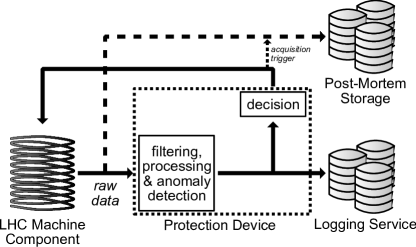
Figure 9: Currently used system.

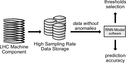
Figure 10: Data acquisition & model training (offline).

Figure 11: Model testing (offline).

Figure 12: Design flow for future hardware implementation.

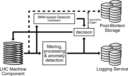
Figure 13: Proposed system.

After the right detector setup is chosen, it can be integrated into (in CERN use case) magnets protection and monitoring system. The currently used conventional system comprises, among others, hardware modules and a set of databases, as shown in Fig. 9.

Voltage and current signals in powering circuits of magnets are acquired with high sampling rate (see subsection 2.2). Obtained raw data is then preprocessed and filtered in real-time, finally arriving in discriminating and thresholding module. This module allows discerning whether a situation arose that needs running automatic fail-safe procedures and an expert intervention. Described conventional solution highly depends on the expert knowledge concerning behavior and parameters of the LHC magnets and associated equipment, which allows selecting monitoring system hyper-parameters.

Only every $n$-th sample of raw data is stored in CALS database, where symbol $n$ denotes a decimation factor. In actual operational scenarios there is no possibility to store all acquired data due to limited network bandwidth. However the data collected in the CALS database allows for later analysis and reasoning about LHC equipment condition and behavior. In case of trigger generation by the discriminating and thresholding module a set of samples stored in the protection device is transmitted as Post Mortem data and is stored in dedicated database. An original sampling rate or low decimation factor is used in this case allowing better insight into an event.

Fig. 10 and 11 show offline model training and testing. The target system should use data acquired with highest possible sampling rate to ensure the required system reaction time by inferring an anomaly directly inside protection device. For current experiments validating the approach feasibility the logging data (see subsection 2.2) was used. Once the model is trained, it can be periodically updated when even more data is available.

It needs to be highlighted that every kind of magnets will need to have distinct setup. The substantial amounts of data that could be potentially obtained should allow to very effectively train the required models. It is expected that a single model instance should be sufficient for all magnets belonging to one category. However, it will need to be verified experimentally.

The current research is focused on validation and quality evaluation of models implemented in a high-level language. However, once the detector setup is determined and model fitted, the anomaly detection algorithm will need to be implemented in hardware, for example using FPGA platforms, to meet latency constraints (see Fig. 12).

Such an implementation poses several challenges that will not be widely discussed in this paper. However, it needs to be noted that fitting the detector system inside an FPGA platform that has limited computing and memory resources will require model compression. It also translates to the constraints on the model size - the smaller number of model parameters (weights), the better. For that reason, the underlying model hyper-parameters optimization needs to take the resources availability into account.

Fig. 13 shows the vision of a final MPS, which includes both the proposed RNN-based detector and conventional solution. Such an approach would allow increasing the reliability of the superconducting magnets monitoring system. It is also possible to use only the proposed detector module.

6 Detector design methodology

The presented detector system has a set of hyper-parameters, that can be tweaked to achieve best results for a particular use case. Some of them are directly influenced by the required operation macro-parameters, such as the smallest anomaly length or amplitude change, that the system should be able to detect, or the maximum response latency.

The process of tweaking the detector setup is highly iterative, with future hardware implementation in mind. Optimizing the model to achieve a better accuracy usually comes hand in hand with increasing it resources consumption. As such, contrary to the usual approach, the model underlying the detector, at the beginning very small, should be improved until it is just good enough for the application.

6.1 Generic steps

Algorithm 1 Methodology steps

procedure detector_setup(raw_data, application_quality_requirements)

2:     model, analyzer, detector, preprocess_config $\leftarrow$ create()

     train_data, test_data $\leftarrow$ preprocess_data(raw_data, preprocess_config)

4:     decimated_data $\leftarrow$ decimate_data(train_data)

     model.fit(decimated_data)

6:     train_prediction $\leftarrow$ model.predict(train_data)

     train_anomalies $\leftarrow$ analyzer.detect(train_data, train_prediction)

8:     thresholds $\leftarrow$ analyzer.auto_thresholds(train_anomalies)

     analyzer.apply(thresholds)

10:     test_prediction $\leftarrow$ model.predict(test_data)

     test_anomalies $\leftarrow$ analyzer.detect(test_data, test_prediction)

12:

     while detector.quality < application_quality_requirements do

14:         if is_oversensitive(model) then

              thresholds++

16:         else

              best_thresholds $\leftarrow$ thresholds

18:              models $\leftarrow$ generate_candidate_setup(model, preprocess_config)

              for all candidate_model $\in$ models do

20:                  train_data, test_data $\leftarrow$ preprocess_data(raw_data, preprocess_config)

                  decimated_data $\leftarrow$ decimate_data(train_data)

22:                  candidate_model.fit(decimated_data)

                  train_prediction $\leftarrow$ candidate_model.predict(train_data)

24:                  train_anomalies $\leftarrow$ analyzer.detect(train_data, train_prediction)

                  candidate_thresholds $\leftarrow$ analyzer.auto_thresholds(train_anomalies)

26:                  if candidate_thresholds < best_thresholds then

                       best_candidate $\leftarrow$ candidate_model

28:                       best_thresholds $\leftarrow$ candidate_thresholds

                  end if

30:              end for

              model $\leftarrow$ best_candidate

32:              analyzer.apply(best_thresholds)

              test_prediction $\leftarrow$ model.predict(test_data)

34:              test_anomalies $\leftarrow$ analyzer.detect(test_data, test_prediction)

         end if

36:     end while

38:     return detector

end procedure

In the initial phase (Alg. 1, lines 2–11), the data is preprocessed (normalized, quantized, formatted according to model needs and split into training and testing sets) and, if possible and to reduce computation time, decimated.

Next, the starting model is fitted with decimated data and then used to make predictions on the training set. Predictions obtained from the model are then used by the analyzer to detect anomalies.

Since anomalies are detected in training set (where target system should report none), they can be used to adjust analyzer thresholds automatically. Procedure for automatic thresholds and rules selection is described in the following subsection. Finally, the model is used to make predictions on testing data, which are then used for anomaly detection.

The iterative phase (Alg. 1, lines 13–36) starts with detector quality evaluation (using Precision, Recall and F-score metrics, see subsection 7.3). Exact quality evaluation depends on application needs, e.g., there can be applications where a lower number of false positives is more important than a lower number of false negatives.

If an amount of false positives is high and real anomalies are (using measures like a length or a cumulative amplitude) bigger than those incorrectly reported anomalies, the model can be considered as oversensitive. This situation can be addressed by increasing analyzer threshold values, especially those where the gap between real true and false anomalies is significant.

If thresholds adjustment is impossible (e.g., true anomalies measurements are similar to those of false anomalies, or the model is not accurate enough, resulting in high false negatives number), the only way to improve the detector quality is by changing the preprocessing or improving the underlying model.

After setup is improved, the detector quality evaluation can begin anew.

6.2 Automatic rules adjustment

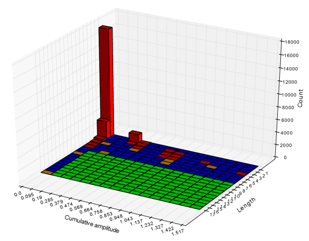
Figure 14: Example chart showing false anomalies in first 200k training samples; saved area marked in green.

Algorithm 2 Automatic thresholds and rules selection

procedure analyzer.auto_thresholds(train_anomalies)

2:     possible_thresholds $\leftarrow$ supported_thresholds()

     for all threshold $\in$ possible_thresholds do

4:         maxima[threshold] $\leftarrow$ max(train_anomalies[threshold])

         best_combination[threshold] $\leftarrow$ 0

6:         bins[threshold] $\leftarrow$ compartmentalize(train_anomalies[threshold])

     end for

8:     best_combination[possible_thresholds[0]] $\leftarrow$ maxima[possible_thresholds[0]]

     best_area $\leftarrow$ 0

10:     possible_combinations $\leftarrow$ combine(bins, possible_thresholds)

     for all combination $\in$ possible_combinations do

12:         is_valid_combination $\leftarrow$ true

         for all anomaly $\in$ train_anomalies do

14:              if above_thresholds(anomaly, combination) then

                  is_valid_combination $\leftarrow$ false

16:                  break

              end if

18:         end for

         if is_valid_combination then

20:              area $\leftarrow$ calculate_saved_area(combination, maxima)

              if area > best_area then

22:                  best_area $\leftarrow$ area

                  best_combination $\leftarrow$ combination

24:              end if

         end if

26:     end for

     rules $\leftarrow$ []

28:     for all threshold $\in$ possible_thresholds do

         if best_combination[threshold] > 0 then

30:              rules.push(threshold)

         end if

32:     end for

     return best_combination, rules

34:end procedure

The proposed automatic analyzer rules selection procedure, described in Alg. 2, is conceptually simple. Its objective is to find such a combination of threshold values that will guarantee filtering out all false anomalies found in training set. At the same time, it should not be too greedy, in case true anomalies are close to false ones.

For example, most of the false anomalies can be shorter than a certain length, while at the same time spanning full cumulative amplitude range. Simultaneously, there can exist a small number of long false anomalies which are low in cumulative amplitude. It can be then surmised that any longer (but still within range) anomaly with higher (in range) cumulative amplitude would be a true one and should not be filtered out. If only greedy, essential thresholds were applied (,,anomaly is true if its length or cumulative amplitude or amplitude is bigger than the relevant maximum found for false anomalies”), the anomaly as mentioned earlier would not match any of those criteria and therefore would not be detected.

In Fig. 14, the example visualization of false anomaly properties is shown. It is a 2-D histogram, with an amount of bins equal to the amount of possible discrete values (for small anomaly length ranges) or calculated using numpy ’sturges’ algorithm [62]. Assuming there are only two thresholds possible (length and cumulative amplitude, for example), the algorithm task is to find such values, that will result in the largest possible saved area (marked in green in Fig. 14). The saved area represents an additional space (aside from areas beyond the found maximums) in which anomaly detection will be possible. This reasoning is then generalized to an arbitrary number of parameters.

Initially, the algorithm sets the best threshold combination to contain a value only for the first threshold, with others set to $0$. The first threshold value is based on the maximum value appearing in anomalies, and the saved area is set to $0$ (Alg. 2, lines 1–9).

In the next part, possible threshold combinations are checked (Alg. 2, lines 10–26). For every detected anomaly, it is checked if a particular threshold combination can be used to filter it out. If the combination can be used to filter all anomalies, it is considered valid and saved area for that particular combination is calculated. The best threshold combination is the one with the highest saved area.

6.3 Setup improvement

A crucial part of improving detector setup is selecting the optimum underlying model (Alg. 1, lines 18–31). The number of NN models hyper-parameters optimization methods is rapidly growing, starting with the heuristic-based approaches and moving toward ones utilizing RL (Reinforcement Learning) and Bayesian algorithms [63, 64, 65, 66]. The description of those approaches is beyond the scope of this paper, but it needs to be pointed out that most of those algorithms are not created with hardware implementation in mind. The authors are researching an automatic, resource-aware NN models hyper-parameters optimization, the preliminary concept of which is described in [67], to address this issue.

7 Experiments

The experiments with both evenly-spaced grid and adaptive one were conducted and compared with the standard SVM (Support Vector Machine)-based solution. Collected results allowed to judge the effectiveness and efficiency of the proposed solution.

7.1 Dataset

Table 6: Properties of the used dataset.

	samples (in millions)
series	training	testing	total
h1144	$\sim 3.8$	$\sim 1.2$	$\sim 5$
h1011	$\sim 5.1$	$\sim 0.4$	$\sim 5.5$
h1451	$\sim 4.5$	$\sim 0.5$	$\sim 5$
h1819	$\sim 5.7$	$\sim 0.3$	$\sim 6$

The data used in the experiments were acquired during HiLumi (High Luminosity) magnets training. However, the developed methods will also be applicable during the normal machine operation (during the LHC cycle, when the magnet works at the nominal current). Those magnets are still in a testing and training phase, with their characteristics being checked and operation parameters verified.

The magnet training consists of repeated magnet runs during which the current is slightly increased until they quench under control, with the aim of stabilizing the magnet at its design specification (ultimate current). The data was obtained from the short model of the $11\text{\,}\mathrm{T}$ dipole magnet (MBHSP105) with a single aperture (see subsection 2.2 for detailed description). Each of the series contains four data channels, with first two representing the voltages on magnet coils, third - the current measurement and fourth - the compensated signal (sum of the first two) (Fig. 3).

To obtain actual voltage values from the signals, they need to be multiplied by gain of analogue stage $G~{}=~{}$5\text{\,}\mathrm{V}\text{/}\mathrm{V}$$ and conversion factor of ADC $\mathit{LSB}~{}=~{}$9.5348\text{\,}\mathrm{\SIUnitSymbolMicro V}\text{/}\mathrm{bit}$$. The current signal is acquired from the voltage output of the DCCT (Direct-Current Current-Transformer) installed on the power converter, and the related value is obtained multiplying the voltage signal from the DCCT by a conversion factor of $2\text{\,}\mathrm{kA}\text{/}\mathrm{V}$. For the experiments, only the first three channels were used.

The collected data is divided into four series (h1011, h1144, h1451 and h1819), all coming from the same magnet during the different training runs. Each of the series contains an extended period of the normal operation (ramp up of the magnet), followed by an anomaly (quench) and results of a power abort procedure.

Each of the series was then split into two parts, one containing only normal operation data (training set) and the second one containing the anomaly and power abort in addition to normal operation (testing set; see Tab. 6 for details).

Both the quenches and the power abort fragments were annotated as anomalies when measuring the detector performance since both contain phenomena that the model has never seen.

Since there are only a few real anomalies available, to further examine the detector performance, the tests sets containing synthetic anomalies were created. For that purpose, the normal operation part of h1011 series was augmented with a thousand of synthetic anomalies added.

In the synthetic set I, introduced anomaly is a unit step impulse with the duration of $100$ samples (see Fig. 20 and 21). The synthetic set II is similar, only with unit step impulse duration set to $50$ samples.

7.2 Preprocessing

The acquired data needs to be initially prepared to be used for recurrent neural network training. The first step is the signals normalization to $[0,1]$ range, using all of the available data. The normalized data is saved to be reused in all the experiments. Normal operation data is used for model training and validation, while data containing anomalies and power abort is used for complete detector setup testing.

In the next step, based on $\mathtt{in\_grid}$, $\mathtt{out\_grid}$, $\mathtt{in\_algorithm}$ and $\mathtt{out\_algorithm}$ configuration values, the grid edges are calculated. They will later be used to quantize input and output signals.

Following that the data structuring is done. For all the data points that have the required history length (the sample index in series is greater than or equal to $\mathtt{look\_back}$ + $\mathtt{look\_ahead}$) tensors containing that history (with $\mathtt{look\_back}$ length) for all three used channels are created. At the same time, this historical data is quantized, using previously calculated edges. It needs to be highlighted that, unlike when working with statistical models such as SVM, the data used for training is overlapping. Simultaneously, the output data tensor using ’one hot’ encoding is created, with length equal to the $\mathtt{out\_grid}$ parameter. Voltage 0 signal was selected as the prediction target.

After history tensors and linked output categories are prepared for each data series, they are all mixed. For the actual experiment, a fraction of data specified by the $\mathtt{samples\_percentage}\in[0,1]$ is randomly chosen.

7.3 Quality measures

Several standard quality measures were used to compare models and detector setups, as well as compare proposed solution performance with alternative approaches.

7.3.1 Model quality

The metric used for measuring the underlying GRU model is accuracy. Given the values $t$ and $f$ representing, respectively, an amount of correctly and incorrectly classified samples, the accuracy can be defined as in (11):

$$\mathrm{accuracy}=\frac{\mathit{t}}{\mathit{t}+\mathit{f}}.$$ (11)

7.3.2 Detector quality

A switch from measuring the quality on a per-sample basis to a per-anomaly basis is needed to score the detector performance. This need is especially true considering the rarity of anomalies, where the number of samples belonging to the ’anomaly’ category is insignificant when compared with the number of normal operation samples. In such a case, any metric incorporating total number of samples (like accuracy) would not provide any meaningful information about anomaly detection capabilities.

Scoring the performance on a per-anomaly basis, on the other hand, needs some well-defined rules for the metrics to be useful. The most straightforward question that needs to be answered is ,,when the detected anomaly (positive) is considered true?”. In this paper, a detected anomaly is considered to be true positive if any part of it overlaps with the real anomaly. What follows, if several detected anomalies are overlapping a single real one, all of them are considered true. This behavior also occurs in reverse, if a single detected anomaly spans several real ones, all of them are considered to be found.

Depending on the application needs, it may be crucial to be able to qualify the detection quality further. An attempt to develop the more comprehensive anomaly detection metrics can be found for example in [68].

It needs to be noted that, due to continuous nature of detector operation, it is impossible to define a true negative. Such a notion would not only require artificial splitting of time series into windows of arbitrary length and overlap but also contradicted the purpose of the switch from per-sample based metrics to per-anomaly ones. This lack of true negatives narrows down the available standard quality measures.

The selected quality metrics should reflect the application needs. In case of the HiLumi data, it is crucial to find all anomalies, since undetected faults may lead to huge disaster in the LHC tunel and in the consequence costly repairs and long accelerator shutdowns. On the other hand, false positives reflect the machine availabilty which is a crucial operational parameter of the accelerator. The two metrics, measuring those features, are recall (12), also called sensitivity, and precision (13), respectively:

$$\mathrm{recall}=\frac{\mathit{tp}}{\mathit{tp}+\mathit{fn}},$$ (12)

$$\mathrm{precision}=\frac{\mathit{tp}}{\mathit{tp}+\mathit{fp}},$$ (13)

where:

• $\mathit{tp}$ – true positive – item correctly classified as an anomaly,

• $\mathit{fp}$ – false positive – item incorrectly classified as an anomaly,

• $\mathit{fn}$ – false negative – item incorrectly classified as a part of normal operation.

To combine those two metrics into a single one that can be directly applied for anomaly detection solutions comparison, an F-measure is used (14). The $\beta$ parameter controls the recall importance in relevance to the precision:

$$\mathrm{F}_{\beta}=(1+\beta^{2})\cdot\frac{\mathrm{recall}\cdot\mathrm{precision}}{\mathrm{recall}+\beta^{2}\cdot\mathrm{precision}}.$$ (14)

During the detector performance experiments two $\beta$ values were used, $1$ and $2$, to show the impact of the recall on the final score.

7.4 Methodology validation

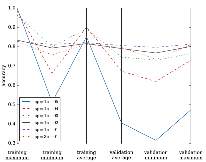
Figure 15: Influence of $\mathtt{samples\_percentage}$ ($\mathtt{sp}$) on model accuracy ($\mathtt{look\_back}$=10, $\mathtt{in\_grid}$=10, $\mathtt{out\_grid}$=10, average over various $\mathtt{cells}$ values).

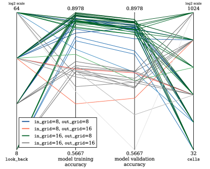
Figure 16: Influence of $\mathtt{look\_back}$ and $\mathtt{cells}$ on model accuracy for various $\mathtt{in\_grid}$ and $\mathtt{out\_grid}$ combinations ($\mathtt{samples\_percentage}$=0.01). Darker colors indicate higher model validation accuracy.

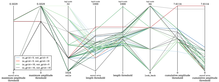
Figure 17: Influence of $\mathtt{look\_back}$ and $\mathtt{cells}$ on automatically calculated thresholds ($\mathtt{samples\_percentage}$=0.01). Darker colors indicate bigger model (bigger $\mathtt{cells}$ values). See Tab. 7 for statistics.

Table 7: Automatically calculated thresholds statistics.

threshold	min	max	median	mean
length	14	918	29.5	56
saved area length	1	108	12	19.76
cumulative amp.	2.28	7.61	3.79	3.92
saved area cumulative amp.	0	7.61	1.01	1.3
maximum amplitude	0.38	0.5	0.5	0.49
saved area maximum amplitude	0	0.39	0	0.07

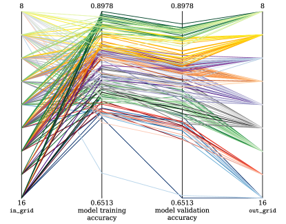
Figure 18: Influence of grid sizes on model accuracy ($\mathtt{look\_back}$=32, $\mathtt{samples\_percentage}$=0.01). Darker color shades indicate bigger $\mathtt{in\_grid}$, while colors themselves signify $\mathtt{out\_grid}$ values.

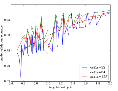
Figure 19: Influence of grid sizes ratio on model accuracy ($\mathtt{look\_back}$=32, $\mathtt{samples\_percentage}$=0.01).

Experiments involving neural networks are usually very resource-consuming. To reduce computational cost, it may be beneficial to at first train model on (small) representative fraction of available training data. A random sweep with increasing percentage values was conducted to select such a percentage used in later experiments. The sweep results can be seen in Fig. 15. The data fraction can be considered to be big enough when, for a given model, training and validation accuracy is similar. Based on the experiment results, it can be seen that the above condition is true starting with $1\text{\,}\mathrm{\char 37\relax}$ of the original dataset size ($\mathtt{samples\_percentage}$=0.01) – in the visualization, the line connecting those two accuracy values is nearly horizontal. Moreover, the relative difference between average accuracy achieved for higher $\mathtt{samples\_percentage}$ values is minimal. Therefore, the $1\text{\,}\mathrm{\char 37\relax}$ value was determined to be sufficient for the following tests.

Fig. 16 shows the relationship between four hyper-parameters: history window length ($\mathtt{look\_back}$), number of GRU model cells and $\mathtt{in\_grid}$/$\mathtt{out\_grid}$ values. It can be observed that model performance mainly depends on grid sizes (with best results achieved for $\mathtt{in\_grid}$=16 and $\mathtt{out\_grid}$=8), with $\mathtt{look\_back}$ and model size ($\mathtt{cells}$) values having a surprisingly small impact. It is, however, worth noting that smaller models with smaller $\mathtt{look\_back}$ values tend to have better performance than those with one of the parameters closer to the upper tested limit.

Fig. 17 visualizes relationships between $\mathtt{look\_back}$, model validation accuracy, and calculated threshold parameters. The grids sizes influence on length and cumulative amplitude thresholds is small, but noticeable, especially affecting maximum false anomaly length, which in turns affects saved area length threshold. The $\mathtt{look\_back}$ values seem to play a significant role in determining model capabilities – smaller values tend to result in lower maximum false anomalies length. It can also be seen that maximum false anomaly amplitude (topping up around $0.5$) depends almost entirely on $\mathtt{out\_grid}$.

As an additional experiment, authors conducted a more thorough research into the impact of grid sizes on model accuracy (Fig. 18 and 19). It turns out that $\mathtt{in\_grid}$/$\mathtt{out\_grid}$ ratio is very visibly related to model accuracy, with lower ratio values lowering the model performance. However, if the higher ratio cannot be achieved, it is better to use lower $\mathtt{out\_grid}$ value.

7.5 Detector performance

Table 8: Detector performance results.

		Setup
		$\mathtt{best\_length}$	$\mathtt{best\_cum\_amp}$	$\mathtt{best\_max\_amp}$	$\mathtt{best\_accuracy}$	$\mathtt{balanced}$
Parameters	$\mathtt{in\_grid}$	16	8	16	16	16
	$\mathtt{out\_grid}$	8	8	16	8	8
	$\mathtt{look\_back}$	16	16	16	32	8
	$\mathtt{cells}$	64	64	512	64	64
Model accuracy	train	0.8955	0.8828	0.7634	0.8978	0.8756
	validation	0.8809	0.8654	0.7553	0.8812	0.8551
False anomalies maximums	$\mathtt{length}$	14	24	38	24	29
	$\mathtt{cum\_amp}$	3.4104	2.2761	3.7890	3.4110	3.4110
	$\mathtt{max\_amp}$	0.5026	0.5026	0.3824	0.5026	0.5026
Saved area thresholds	$\mathtt{length}$	10	9	20	14	11
	$\mathtt{cum\_amp}$	1.5503	1.5520	1.6474	0.7755	0.7755
	$\mathtt{max\_amp}$	0	0	0	0	0
Real set	recall	1.0	1.0	1.0	1.0	1.0
	precision	1.0	0.0046	0.0005	1.0	1.0
	$\mathrm{F}_{1}$	1.0	0.0091	0.0009	1.0	1.0
	$\mathrm{F}_{2}$	1.0	0.0225	0.0023	1.0	1.0
Synthetic set I	recall	0.9974	0.9950	0.6848	0.9979	0.8312
	precision	1.0	1.0	1.0	0.9986	1.0
	$\mathrm{F}_{1}$	0.9987	0.9975	0.8129	0.9982	0.9078
	$\mathrm{F}_{2}$	0.9979	0.9960	0.7309	0.9980	0.8602
Synthetic set II	recall	0.8685	0.8184	0.4340	0.8643	0.5045
	precision	1.0	0.9988	1.0	0.9977	1.0
	$\mathrm{F}_{1}$	0.9296	0.8996	0.6053	0.9262	0.6706
	$\mathrm{F}_{2}$	0.8920	0.8490	0.4894	0.8880	0.5600

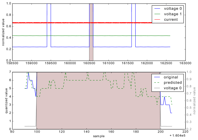
Figure 20: False negative (samples 160500 – 160600) anomaly in synthetic set I missed by $\mathtt{best\_accuracy}$ detector setup.

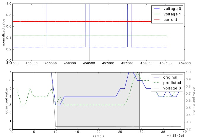
Figure 21: False positive (samples 456501 – 456520) anomaly in synthetic set I found by $\mathtt{best\_accuracy}$ detector setup.

Five of the setups were selected using different criteria to test detector performance:

• $\mathtt{best\_length}$ – setup with the lowest maximum false anomaly length,

• $\mathtt{best\_cum\_amp}$ – the lowest maximum false anomaly cumulative amplitude,

• $\mathtt{best\_max\_amp}$ – the lowest maximum false anomaly amplitude,

• $\mathtt{best\_accuracy}$ – the highest model validation accuracy

• $\mathtt{balanced}$ – setup with relatively good accuracy, low maximum values of length and cumulative amplitude, as well as saved area length and cumulative amplitude thresholds.

Exact setup parameters, as well as performance results, are described in Tab. 8.

Looking only at the results on the real data test set, it may seem that $\mathtt{best\_length}$, $\mathtt{best\_accuracy}$, and $\mathtt{balanced}$ setups perform equally well. The performance of the $\mathtt{best\_cum\_amp}$ and $\mathtt{best\_max\_amp}$ ones is abysmal, which outright disqualifies them from being used with this particular data.

Looking at the results for test sets containing unit step impulses, however, brings out a bit different picture. The $\mathtt{balanced}$ setup is not performing nearly as well, with a significant drop in the recall value even for long impulses and meager score for shorter ones. The $\mathtt{best\_length}$ setup scores are still very high, with $\mathtt{best\_accuracy}$ ones slightly outperforming it regarding recall and $\mathrm{F}_{2}$ for longer impulses.

Fig. 20 shows the example of false negative, missed by the $\mathtt{best\_accuracy}$ setup in synthetic set I. When predicted and real quantized anomaly values in the selected section of the signal are compared, it can be seen that in several points the predicted values fall into the highest range. From the detector point of view it means that the model, after some small error, correctly predicted current value, and the anomaly candidate can be disregarded. Such a situation occurs as a result of the discriminating thresholds being too high in this particular case.

One of the ways in which this problem possibly may be mitigated is an $\mathtt{out\_grid}$ increase. Direct application of this solution, however, severely affects the model accuracy (as shown in Fig. 18) – $\mathtt{out\_grid}$ increase needs to come in hand with other parameters, especially $\mathtt{in\_grid}$, adjustment.

Another way involves changing the way analyzer confirms or rejects anomaly candidates. As mentioned, currently candidate is rejected whenever a true prediction is made, unless the configured thresholds were passed first. An alternative approach, subject to future research, could involve tracking a ratio of true vs. false predictions or introducing required true predictions threshold for candidate rejection.

Fig. 21 shows the example false positive, found in the synthetic set I using the $\mathtt{best\_accuracy}$ setup. It can be seen that the false positive was reported soon after the synthetic anomaly occurred, so it can be assumed that incoming anomalous signal affected the model predictions. In the real-world scenario, this should not be a problem, since first detected anomaly would probably trigger a failsafe mechanism. In cases where anomalies should be detected even if they occur one after another, a solution involving a small ignored window, equal in length to a half or a whole $\mathtt{look\_back}$ value, could probably be implemented. How such a mechanism would affect the whole detector performance needs to be researched.

Overall, it seems that for HiLumi data analysis, the setups selected based on the lowest maximum false anomaly length may yield the best performance, with the ones based on best accuracy being nearly as good.

7.6 Alternative approach: OC-SVM

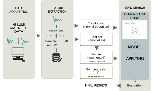
Figure 22: Overall block diagram summarizing the main processing stages and anomaly detector based on OC-SVM.

Several implementations of anomaly detection systems based on OC-SVM were proposed with promising results [33, 34, 35, 36]. These algorithms are trained offline to subsequently work online. In this subsection, the comparison of OC-SVM models with the proposed GRU-based system is presented.

Some properties of the experimental setup needed to be changed as required by the nature of the OC-SVM. Therefore, the HiLumi data was preprocessed accordingly. In following paragraphs the OC-SVM algorithm, the preprocessing and the experimental setup with results are described in the details.

7.6.1 One Class Support Vector Machine

OC-SVMs are a particular case of SVM, that can be trained with unlabeled data. Therefore, they are an example of unsupervised machine learning techniques. In OC-SVM the support vector model is trained on data that has only one class, the ,,normal” class, which infers the properties of normal cases. As such, after training, the examples ,,unlike normal examples” can be detected. In an anomaly detection field, this is especially useful, as there are many different situations where the training examples are scarce (such as fraud detection, or network intrusion).

In the experiments, the OC-SVM by Schölkopf et al. [38, 39] implemented using Sklearn Python library was used. This SVM separates all the data points from the origin (in feature space $F$) and maximizes the distance from this hyperplane to the origin. This operation results in a binary function which captures regions in the input space where the probability density of the data is positioned. In such a way the function returns $+1$ in a ’small’ region (capturing the training data points) and $-1$ elsewhere.

7.6.2 Data preprocessing

Table 9: Properties of training and testing sets used with OC-SVM with respect to the $\mathtt{window\_size}$.

		$\mathtt{window\_size}$
		$1024$	$512$	$128$
Training set samples		$74\,607$	$149\,217$	$596\,875$
Testing set (augmented)	initial no of examples	$9350$	$18\,702$	$74\,812$
	quenches multiplication	$4675$	$9351$	$37\,406$
	final no of examples	$14\,025$	$28\,053$	$112\,218$

The OC-SVM was trained on the normal operation data. As described in subsection 7.1, four series (h1011, h1144, h1451 and h1819) were used, all coming from the same magnet, with only the actual voltage values for each of the signals used in experiments. Each of the series was then split into two parts: a training set, containing only normal operation data and a testing set containing the anomalies.

The sets were then preprocessed and various features extracted, similar to [36], to achieve a simpler classifier. The extracted features and their properties are represented in B in Tab. 12. Tab. 9 shows different $\mathtt{window\_size}$ values (in samples) which were used for extracting the features and the resulting training and testing sets.

7.6.3 Training and testing

Table 10: OC-SVM performance results.

		$\mathtt{window\_size}$
		$1024$	$512$	$128$
Training set	accuracy	$0.94$	$0.98$	$0.99$
	recall	$1.0$	$1.0$	$1.0$
	precision	$1.0$	$1.0$	$1.0$
	$\mathrm{F}_{1}$	$1.0$	$1.0$	$1.0$
	$\mathrm{F}_{2}$	$1.0$	$1.0$	$1.0$
Testing set (augmented)	accuracy	$0.92$	$0.92$	$0.87$
	recall	$1.0$	$1.0$	$1.0$
	precision	$1.0$	$1.0$	$1.0$
	$\mathrm{F}_{1}$	$1.0$	$1.0$	$1.0$
	$\mathrm{F}_{2}$	$1.0$	$1.0$	$1.0$
Synthetic set I	accuracy	$0.72$	$0.85$	$0.96$
	recall	$1.0$	$1.0$	$0.84$
	precision	$0.28$	$0.15$	$0.03$
	$\mathrm{F}_{1}$	$0.43$	$0.25$	$0.06$
	$\mathrm{F}_{2}$	$0.66$	$0.46$	$0.13$
Synthetic set II	accuracy	$0.74$	$0.87$	$0.95$
	recall	$1.0$	$1.0$	$0.88$
	precision	$0.26$	$0.13$	$0.04$
	$\mathrm{F}_{1}$	$0.42$	$0.23$	$0.08$
	$\mathrm{F}_{2}$	$0.64$	$0.43$	$0.19$

OC-SVM, using RBF (Radial Basis Function) kernel, was trained on the preprocessed training dataset (the grid search method to find the best values of $\nu$ ($=0.07$) and $\gamma$ ($=0.06$) was used). After training, the model has run on the test datasets where there were data labeled with known quenches. Due to very few numbers of quenches in the test data, the test set has been augmented, increasing the number of quench instances so that it would match normal samples cardinality. Tab. 9 shows the properties of this augmented test set. The model has also run on the same synthetic data sets that were used to validate the GRU-based detector. Fig. 22 summarizes the main processing stages for OC-SVM and contains a high-level description of the methods used in this alternative approach.

Tab. 10 shows the results (following the metrics described in 7.3) of the OC-SVM on the HiLumi data with synthetic data sets.

8 Discussion

To be able to measure the detector system performance, it is necessary to answer the question of what and where an anomaly is in this context. Exact anomaly position is tough to determine when it comes to the signals acquired from the LHC magnets, especially the new HiLumi ones.

The target model should be trained using data acquired with the very high sampling rate, obtained during the experiments with the magnets. This kind of data is not available during normal operation in any database because of limited network throughput. Therefore the target system can be applied only in the immediate vicinity of the signal source, directly on the detecting device located near superconducting component in the LHC tunnel, as it is only place where data is available without any decimation. Hardware implementation (in FPGA or ASIC) is also required to meet the CERN requirement of very low system response latency.

The solution based on NNs was selected because those models may be updated automatically, require minimal feature extraction, can be compressed efficiently and ported into hardware [69, 70, 71].

Choosing the right model for the task and its hyper-parameters adjusting can be a very time- and resource-consuming process. An automation of that process should potentially not only adjust the model hyper-parameters but also address the problem of model compression/precision reduction challenges and therefore make a NN-based solution hardware implementation much more manageable. The currently used at CERN anomaly detection system required the adoption of the high-level models using HDL (Hardware Description Language) (e.g., VHDL). Such an approach results in a complicated and error-prone process. Furthermore, any updates or modifications of the high-level models require a complete reiteration of the design flow. The adaptability of the NN-based system coupled with the automatic optimization algorithm could significantly simplify that process.

It is also worth noting that historically at CERN feature extraction was a challenging phase since it involved many experiments with a range of filtering and discrimination methods to reach reliable parameters of the system as a whole. While the naive adoption of RNNs requires an operator of the system to make an arbitrary decision regarding the values of the thresholds [58], the adaptive inputs and outputs quantization approach presented in this work alleviates this issue by introducing an automatic required analyzer thresholds adjustment process.

9 Conclusions

In this paper, an applicability of RNN models for detecting anomalous behavior of CERN superconducting magnets was examined. The developed solution, based on GRU and adaptive quantization, achieved very encouraging results for the data acquired from HiLumi magnets. Three testing sets were used in the experiments, one including real anomalies and two with synthetic anomalies in the form of a unit step impulse with the length of 100 and 50 samples. For those datasets, the proposed anomaly detection system reached $\mathrm{F}_{2}$ equal to $1.0$, $0.9980$, and $0.8920$, respectively, with $\mathrm{F}_{1}$ equal to $1.0$, $0.9987$, and $0.9296$. Several setups of the proposed solution were analyzed, with the configurations selected based on shortest reported false anomaly length and best underlying model accuracy achieving the best results.

An essential part of the proposed solution is the adaptive quantization algorithm. It can convert 20-bits input samples to reduced (e.g., 4-bits) representation that can be used as the model input. The input and output quantization parameters turned out to have a significant impact on the detector performance, with 16/8 ratio providing the best overall results among the tested cases. Another noteworthy aspect of the developed anomaly detector is specially designed analyzer which processes anomalies’ candidates.

Despite being primarily focused on the CERN equipment monitoring, the results presented in this paper should be considered a part of a larger endeavor aiming at developing a methodology and architecture of an anomaly detection system operating in the space of time series analysis, especially under hard real-time constraints.

10 Future work

As a future work, the authors plan to further test and improve the proposed algorithm. It is planned to examine the proposed solution performance using more advanced quality measures and more sophisticated testing datasets and improve adaptive quantization, automatic analyzer rules selection and anomaly discrimination algorithms.

Data with even higher sampling rate will be used. It is worth noting that this data contains even more significant noise component produced by power converters delivering current to coils. It can also contain other fast physical phenomena (flux jumping) that can take place inside a superconductor. Correct anomaly detection must be performed despite these phenomena. Further research can be done regarding a possibility of early warnings (before anomaly) and the existence of quench precursors.

Ultimately, the authors plan to develop an RL-based NN model optimization algorithm, the preliminary idea of which was presented in [67], and use it to simplify the process of the detector prototype implementation on an FPGA platform.

Appendix A Software symbols

Table 11: Software symbols used in the text.

Section	Variable name	Description
data preprocessing	$\mathtt{look\_back}$	the history window length
	$\mathtt{look\_ahead}$	the gap between last historical sample and predicted one; in presented experiments $\mathtt{look\_back}$=1 (predict sample immediately following the history)
	$\mathtt{in\_grid}$	the number of input data quantization levels
	$\mathtt{out\_grid}$	the number of output data quantization levels
	$\mathtt{in\_algorithm}$	the input data quantization algorithm, can be static, adaptive (used in presented experiments) or none (no quantization)
	$\mathtt{out\_algorithm}$	analogical to $\mathtt{in\_algorithm}$, but for output data
	$\mathtt{samples\_percentage}$	the percentage of total available data the model is trained on; it is determined during preprocessing and all following model and analyzer instances are using the same subset
model	$\mathtt{cells}$	the number of GRU model cells; presented experiments utilized only single GRU layer, but it is possible to specify more
analyzer	length threshold†	an anomaly candidate length (in samples) that qualifies it as an anomaly
	maximum amplitude threshold†	an anomaly candidate maximum amplitude (measured as a distance between real and predicted sample quantization bin middles) that qualifies it as an anomaly
	cumulative amplitude threshold†	sum of anomaly candidate amplitudes that qualifies it as an anomaly

The Tab. 11 summarizes the names used in the developed software [6] and useful for understanding this text.

Appendix B Statistical parameters

Table 12: Feature extractors used for OC-SVM [36, 37]. The input signal is denoted as $x[n]$, where $n=\{1,2,\dots,N=\mathtt{window\_size}\}$.

Feature	Equation	Description
Average Power	$\overline{P}=\frac{1}{N}\sum_{n=1}^{N}x[n]^{2}$	overall vibration intensity of the window
Mean Value	$\overline{x}=\sum_{n=1}^{N}x[n]$	amplitude of low frequency
Median frequency	$MF=\begin{cases}(\frac{n+1}{2})&\mbox{if }n\equiv odd\\ \frac{(\frac{n}{2})+(\frac{n+1}{2})}{2}&\mbox{if }n\equiv even\end{cases}$	frequency of the power spectrum into two halves with the same energy [37]
Standard deviation	$\sigma=\sqrt{\frac{1}{N-1}\sum_{n=1}^{N}(x[n]-\overline{x})^{2}}$	shape of the signal
Skewness	$s_{o}=\frac{\sqrt{N(N-1)}}{N-2}\frac{\frac{1}{N}\sum_{n=1}^{N}(x[n]-\overline{x})^{3}}{\left(\sqrt{({1}{N}\sum_{n=1}^{N})(x[n]-\overline{x})^{2}}\right)^{3}}$	reflects asymmetries
Kurtosis	$k_{o}=\frac{N-1}{(N-2)(N-3)}\left((N+1)k_{1}-3(N-1)\right)+3$, where $k_{1}=\frac{\frac{1}{N}\sum_{n=1}^{N}(x[n]-\overline{x})^{4}}{\left(\frac{1}{N}\sum_{n=1}^{N}x[n]-\overline{x})^{2}\right)^{2}}$	peakedness of the histogram
Central Tendency Measurement	CTM $=$ first-order differences on scatter plot representing $x[n+1]-x[n]$ on the X axis against $x[n+2]-x[n+1]$ on the Y axis	randomness of the signal, low value implies sharp changes
Correlation coefficient	$r=\frac{\sum_{n=1}^{N-2}(X[n]-\overline{X})(Y[n]-\overline{Y})])}{\sqrt{\sum_{n=1}^{N-2}(X[n]-\overline{X})^{2}}\sqrt{\sum_{n=1}^{N-2}(Y[n]-\overline{Y})^{2}}}$	unpredictability of the signal from previous data; correlation between the first-order differences of scatter plot with the Pearson’s linear correlation
Lempel-Ziv Complexity	$LZC=\frac{L(N)}{N}$ where $L(N)\equiv$ length of the encoded sequence	characterizes the average information quantity within a window [37]

The Tab. 12 list well-known statistical parameters. In this study they were applied for feature extraction in reference approach based on OC-SVM method.

Appendix C GRU

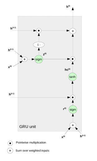
Figure 23: Architecture of GRU unit.

The GRU has gating components which modulate the flow of information within the unit, as presented in Fig. 23. In the related equations (15) to (20) a sigmoidal function is denoted by symbol $\sigma$, and an hyporbelic tangent is denoted as $\phi$.

$$h^{(t)}=(1-z^{(t)})\odot h^{(t-1)}+z^{(t)}\odot hc^{(t)}.$$ (15)

The activation of the model at a given time $t$ is a linear interpolation between the activation $h^{(t-1)}$ from the previous time step and the candidate activation $hc^{(t)}$. It is desribed by equation (15) above. The activation is strongly modulated by quantity $z^{(t)}$ as given by (16) and (17):

$$\begin{split}h^{(t)}&=(1-z^{(t)})\odot h^{(t-1)}+z^{(t)}\odot hc^{(t)}\\ &=h^{(t-1)}-z^{(t)}\odot h^{(t-1)}+z^{(t)}\odot hc^{(t)},\end{split}$$ (16)

$$h^{(t)}=h^{(t-1)}-z^{(t)}\odot(h^{(t-1)}+hc^{(t)}).$$ (17)

$$z^{(t)}=\sigma(W_{zx}x^{(t)}+W_{zh}h^{(t-1)}).$$ (18)

The formula for the update gate is given by (18) and modulates a degree to which a GRU unit updates its activation. The GRU has no mechanism to control to what extent its state is exposed, but it exposes the whole state each time.

$$r^{(t)}=\sigma(W_{rx}x^{(t)}+W_{rh}h^{(t-1)}).$$ (19)

The response of the reset gate is computed according to the same principle as the update gate. The previous state information $h^{(t-1)}$ is multiplied by the coefficients matrix $W_{rh}$ and the input data $x^{(t)}$ is multiplied by the coefficients matrix $W_{rx}$ as shown in (19).

$$hc^{(t)}=\phi(W_{hh}r^{(t)}\odot h^{(t-1)}+W_{hx}x^{(t)}).$$ (20)

The candidate activation $hc^{(t)}$ is computed according to (20). When $r^{(t)}$ is close to 0 (meaning that the gate is almost off), the stored state is forgotten. The input data $x^{(t)}$ is read instead.

As it was pointed out, GRU has a simpler structure than LSTM [58, 59] which is also reflected in the performance of the algorithm.

References

- [1] L. Evans, P. Bryant, LHC Machine, Journal of Instrumentation 3 (08) (2008) S08001. doi:10.1088/1748-0221/3/08/S08001.
- [2] High-Luminosity Large Hadron Collider (HL-LHC). Preliminary Design Report, Tech. rep., CERN, Geneva (Dec 2015). doi:10.5170/CERN-2015-005.
-
[3]
D. Schultke, Preliminary Collider
Baseline Parameters: Deliverable D1.1, Tech. rep., CERN (Sep 2015).
URL http://cds.cern.ch/record/2059230 - [4] ATLAS Collaboration, Observation of a new particle in the search for the Standard Model Higgs boson with the ATLAS detector at the LHC, Physics Letters B 716 (1) (2012) 1–29. arXiv:1207.7214, doi:10.1016/j.physletb.2012.08.020.
- [5] CMS Collaboration, Observation of a new boson at a mass of 125 GeV with the CMS experiment at the LHC, Physics Letters B 716 (1) (2012) 30 – 61. doi:10.1016/j.physletb.2012.08.021.
- [6] M. Wielgosz. Experiments with anomaly detection in HiLumi data [online, cited 22.09.2017].
- [7] G. Stancari, V. Previtali, A. Valishev, R. Bruce, et al., Conceptual design of hollow electron lenses for beam halo control in the Large Hadron Collider (Feb 2015). arXiv:1405.2033.
- [8] L. Bottura, Cable stability, Proceedings of the CAS-CERN Accelerator School: Superconductivity for Accelerators, Erice, Italy (CERN-2014-005) (2014) 401–451. arXiv:1412.5373, doi:10.5170/CERN-2014-005.401.
- [9] Layout Database [online, cited 10.10.2016].
- [10] Quench Database [online, cited 10.10.2016].
- [11] M. Wilson, Superconducting Magnets, Clarendon Press, Oxford, 1983.
- [12] R. Denz, Electronic systems for the protection of superconducting elements in the LHC, IEEE Trans. Appl. Supercond. 16 (2) (2006) 1725–1728. doi:10.1109/TASC.2005.864258.
- [13] J. Steckert, A. Skoczeń, Design of FPGA-based Radiation Tolerant Quench Detectors for LHC, Journal of Instrumentation 12 (04) (2017) T04005. doi:10.1088/1748-0221/12/04/T04005.
- [14] F. Savary, N. Andreev, G. Apollinari, B. Auchmann, et al., Status of the 11 T Dipole Project for the LHC, IEEE Trans. Appl. Supercond. 25 (3). doi:10.1109/TASC.2014.2375914.
- [15] A. Ballarino, Development of superconducting links for the Large Hadron Collider machine, Supercond. Sci. Technol. 27 (044024). doi:10.1088/0953-2048/27/4/044024.
- [16] R. Denz, E. de Matteis, A. Siemko, J. Steckert, Next Generation of Quench Detection Systems for the High-Luminosity Upgrade of the LHC, IEEE Transactions on Applied Superconductivity 27 (4) (2017) 1–4. doi:10.1109/TASC.2016.2628031.
- [17] A. V. Zlobin, N. Andreev, G. Apollinari, B. Auchmann, et al., Quench Performance of a 1 m Long Single-Aperture 11 T Dipole Model for LHC Upgrades, IEEE Trans. Appl. Supercond. 25 (3).
- [18] V. Chandola, V. Mithal, V. Kumar, Comparative evaluation of anomaly detection techniques for sequence data, in: 2008 Eighth IEEE International Conference on Data Mining, 2008, pp. 743–748. doi:10.1109/ICDM.2008.151.
- [19] V. Chandola, A. Banerjee, V. Kumar, Anomaly detection: A survey, ACM Comput. Surv. 41 (3) (2009) 15:1–15:58. doi:10.1145/1541880.1541882.
- [20] M. A. Pimentel, D. A. Clifton, L. Clifton, L. Tarassenko, A review of novelty detection, Signal Processing 99 (2014) 215 – 249. doi:10.1016/j.sigpro.2013.12.026.
- [21] N. Laptev, S. Amizadeh, I. Flint, Generic and scalable framework for automated time-series anomaly detection, in: Proceedings of the 21th ACM SIGKDD International Conference on Knowledge Discovery and Data Mining, KDD ’15, ACM, New York, NY, USA, 2015, pp. 1939–1947. doi:10.1145/2783258.2788611.
- [22] E. J. Candes, X. Li, Y. Ma, J. Wright, Robust principal component analysis? (Dec 2009). arXiv:0912.3599.
- [23] E. Keogh, J. Lin, A. Fu, Hot sax: efficiently finding the most unusual time series subsequence, in: Fifth IEEE International Conference on Data Mining (ICDM’05), 2005, p. 8. doi:10.1109/ICDM.2005.79.
- [24] H. N. Akouemo, R. J. Povinelli, Probabilistic anomaly detection in natural gas time series data, International Journal of Forecasting 32 (3) (2016) 948 – 956. doi:10.1016/j.ijforecast.2015.06.001.
- [25] H. Zengyou, X. Xiaofei, D. Shengchun, Squeezer: An efficient algorithm for clustering categorical data, J. Comput. Sci. Technol. 17 (5) (2002) 611–624. doi:10.1007/BF02948829.
- [26] M. F. Jaing, S. S. Tseng, C. M. Su, Two-phase clustering process for outliers detection, Pattern Recogn. Lett. 22 (6-7) (2001) 691–700. doi:10.1016/S0167-8655(00)00131-8.
- [27] Z. He, X. Xu, S. Deng, Discovering cluster-based local outliers, Pattern Recognition Letters 24 (9) (2003) 1641 – 1650. doi:10.1016/S0167-8655(03)00003-5.
- [28] L. Duan, L. Xu, Y. Liu, J. Lee, Cluster-based outlier detection, Annals of Operations Research 168 (1) (2009) 151–168. doi:10.1007/s10479-008-0371-9.
- [29] S. Lee, G. Kim, S. Kim, Self-adaptive and dynamic clustering for online anomaly detection, Expert Systems with Applications 38 (12) (2011) 14891 – 14898. doi:10.1016/j.eswa.2011.05.058.
- [30] T. Ahmed, M. Coates, A. Lakhina, Multivariate online anomaly detection using kernel recursive least squares, in: IEEE INFOCOM 2007 - 26th IEEE International Conference on Computer Communications, 2007, pp. 625–633. doi:10.1109/INFCOM.2007.79.
- [31] E. R. Faria, J. a. Gama, A. C. P. L. F. Carvalho, Novelty detection algorithm for data streams multi-class problems, in: Proceedings of the 28th Annual ACM Symposium on Applied Computing, SAC ’13, ACM, New York, NY, USA, 2013, pp. 795–800. doi:10.1145/2480362.2480515.
- [32] E. J. Spinosa, A. P. de Leon F. de Carvalho, J. a. Gama, Olindda: A cluster-based approach for detecting novelty and concept drift in data streams, in: Proceedings of the 2007 ACM Symposium on Applied Computing, SAC ’07, ACM, New York, NY, USA, 2007, pp. 448–452. doi:10.1145/1244002.1244107.
- [33] J. Ma, S. Perkins, Time-series novelty detection using one-class support vector machines, in: Proceedings of the International Joint Conference on Neural Networks, 2003., Vol. 3, 2003, pp. 1741–1745 vol.3. doi:10.1109/IJCNN.2003.1223670.
-
[34]
R. Zhang, S. Zhang, S. Muthuraman, J. Jiang,
One class support
vector machine for anomaly detection in the communication network performance
data, in: Proceedings of the 5th Conference on Applied Electromagnetics,
Wireless and Optical Communications, ELECTROSCIENCE’07, World Scientific and
Engineering Academy and Society (WSEAS), Stevens Point, Wisconsin, USA, 2007,
pp. 31–37.
URL http://dl.acm.org/citation.cfm?id=1503549.1503556 - [35] J. Su, Y. Long, X. Qiu, S. Li, D. Liu, Anomaly Detection of Single Sensors Using OCSVM_KNN, Springer International Publishing, Cham, 2015, pp. 217–230. doi:10.1007/978-3-319-22047-5_18.
- [36] R. Ruiz-Gonzalez, J. Gomez-Gil, F. J. Gomez-Gil, V. Martínez-Martínez, An SVM-Based Classifier for Estimating the State of Various Rotating Components in Agro-Industrial Machinery with a Vibration Signal Acquired from a Single Point on the Machine Chassis, Sensors 14 (11) (2014) 20713–20735. doi:10.3390/s141120713.
- [37] R. Hornero, J. Escudero, A. Fernández, J. Poza, C. Gómez, Spectral and nonlinear analyses of meg background activity in patients with alzheimer’s disease, IEEE Transactions on Biomedical Engineering 55 (6) (2008) 1658–1665. doi:10.1109/TBME.2008.919872.
- [38] B. Schölkopf, R. C. Williamson, A. J. Smola, J. Shawe-Taylor, J. C. Platt, Support vector method for novelty detection, in: Advances in neural information processing systems, 2000, pp. 582–588.
- [39] B. Schölkopf, J. C. Platt, J. C. Shawe-Taylor, A. J. Smola, R. C. Williamson, Estimating the support of a high-dimensional distribution, Neural Comput. 13 (7) (2001) 1443–1471. doi:10.1162/089976601750264965.
- [40] K. J. Hole, Anomaly Detection with HTM, Springer International Publishing, Cham, 2016, pp. 125–132. doi:10.1007/978-3-319-30070-2_12.
- [41] M. Wielgosz, M. Pietroń, Using Spatial Pooler of Hierarchical Temporal Memory to classify noisy videos with predefined complexity, Neurocomputing 240 (2017) 84 – 97. arXiv:1609.03093, doi:10.1016/j.neucom.2017.02.046.
- [42] C. Wang, K. Viswanathan, L. Choudur, V. Talwar, W. Satterfield, K. Schwan, Statistical techniques for online anomaly detection in data centers, in: 12th IFIP/IEEE International Symposium on Integrated Network Management (IM 2011) and Workshops, 2011, pp. 385–392. doi:10.1109/INM.2011.5990537.
- [43] P. Angelov, Anomaly detection based on eccentricity analysis, in: 2014 IEEE Symposium on Evolving and Autonomous Learning Systems (EALS), 2014, pp. 1–8. doi:10.1109/EALS.2014.7009497.
- [44] A. M. Bianco, M. García Ben, E. J. Martínez, V. J. Yohai, Outlier detection in regression models with arima errors using robust estimates, Journal of Forecasting 20 (8) (2001) 565–579. doi:10.1002/for.768.
- [45] J. Ekberg, J. Ylinen, P. Loula, Network behaviour anomaly detection using Holt-Winters algorithm, in: 2011 International Conference for Internet Technology and Secured Transactions, 2011, pp. 627–631.
- [46] N. P. Jouppi, C. Young, N. Patil, D. Patterson, et al., In-Datacenter Performance Analysis of a Tensor Processing Unit (Jun 2017). arXiv:1704.04760.
- [47] Project Catapult [online] (2011) [cited 15.08.2017].
-
[48]
A. M. Caulfield, E. S. Chung, A. Putnam, et al.,
A
Cloud-Scale Acceleration Architecture, IEEE Computer Society.
URL https://www.microsoft.com/en-us/research/wp-content/uploads/2016/10/Cloud-Scale-Acceleration-Architecture.pdf - [49] S. Hochreiter, J. Schmidhuber, Long Short-Term Memory, Neural Comput. 9 (8) (1997) 1735–1780. doi:10.1162/neco.1997.9.8.1735.
- [50] J. Chung, C. Gulcehre, K. Cho, Y. Bengio, Gated Feedback Recurrent Neural Networks (2015). arXiv:1502.02367.
- [51] J. Chung, C. Gulcehre, K. Cho, Y. Bengio, Empirical Evaluation of Gated Recurrent Neural Networks on Sequence Modeling (2014). arXiv:1412.3555.
-
[52]
P. Malhotra, L. Vig, G. Shroff, P. Agarwal,
Long
Short Term Memory Networks for Anomaly Detection in Time Series, in: 23rd
European Symposium on Artificial Neural Networks, Computational Intelligence
and Machine Learning, ESANN 2015, Bruges (Belgium), 2015, Proceedings,
Presses universitaires de Louvain, 2015, pp. 89–94.
URL https://www.elen.ucl.ac.be/Proceedings/esann/esannpdf/es2015-56.pdf - [53] L. Bontemps, V. L. Cao, J. McDermott, N.-A. Le-Khac, Collective Anomaly Detection Based on Long Short-Term Memory Recurrent Neural Networks, in: T. K. Dang, R. Wagner, J. Küng, N. Thoai, M. Takizawa, E. Neuhold (Eds.), Future Data and Security Engineering: Third International Conference, FDSE 2016, Can Tho City, Vietnam, November 23-25, 2016, Proceedings, Springer International Publishing, Cham, 2016, pp. 141–152. doi:10.1007/978-3-319-48057-2_9.
- [54] A. Nanduri, L. Sherry, Anomaly detection in aircraft data using Recurrent Neural Networks (RNN), in: 2016 Integrated Communications Navigation and Surveillance (ICNS), 2016, pp. 5C2–1–5C2–8. doi:10.1109/ICNSURV.2016.7486356.
- [55] E. Marchi, F. Vesperini, F. Eyben, S. Squartini, B. Schuller, A novel approach for automatic acoustic novelty detection using a denoising autoencoder with bidirectional lstm neural networks, in: 2015 IEEE International Conference on Acoustics, Speech and Signal Processing (ICASSP), 2015, pp. 1996–2000. doi:10.1109/ICASSP.2015.7178320.
- [56] E. Marchi, F. Vesperini, F. Weninger, F. Eyben, S. Squartini, B. Schuller, Non-linear prediction with lstm recurrent neural networks for acoustic novelty detection, in: 2015 International Joint Conference on Neural Networks (IJCNN), 2015, pp. 1–7. doi:10.1109/IJCNN.2015.7280757.
- [57] Y. S. Chong, Y. H. Tay, Abnormal Event Detection in Videos using Spatiotemporal Autoencoder (Jan 2017). arXiv:1701.01546.
- [58] M. Wielgosz, A. Skoczeń, M. Mertik, Using LSTM recurrent neural networks for detecting anomalous behavior of LHC superconducting magnets, Nuclear Inst. and Methods in Physics Research, A 867 (2017) 40–50. arXiv:1611.06241, doi:10.1016/j.nima.2017.06.020.
- [59] M. Wielgosz, A. Skoczeń, M. Mertik, Recurrent Neural Networks for anomaly detection in the Post-Mortem time series of LHC superconducting magnets (Feb 2017). arXiv:1702.00833.
- [60] F. Chollet, et al. Keras [online] (2015) [cited 10.10.2016].
- [61] Theano Development Team, Theano: A Python framework for fast computation of mathematical expressions (May 2016). arXiv:1605.02688.
- [62] numpy.histogram [online, cited 22.09.2017].
- [63] B. Zoph, Q. V. Le, Neural architecture search with reinforcement learning (Feb 2017). arXiv:1611.01578.
- [64] I. Bello, B. Zoph, V. Vasudevan, Q. V. Le, Neural optimizer search with reinforcement learning (Sep 2017). arXiv:1709.07417.
- [65] E. Brochu, V. M. Cora, N. De Freitas, A tutorial on bayesian optimization of expensive cost functions, with application to active user modeling and hierarchical reinforcement learning (Dec 2010). arXiv:1012.2599.
- [66] K. Li, J. Malik, Learning to optimize (Jun 2016). arXiv:1606.01885.
- [67] M. Wielgosz, The observer-assisted method for adjusting hyper-parameters in deep learning algorithms (Nov 2016). arXiv:1611.10328.
- [68] A. Lavin, S. Ahmad, Evaluating Real-time Anomaly Detection Algorithms - the Numenta Anomaly Benchmark, in: 2015 IEEE 14th International Conference on Machine Learning and Applications (ICMLA), 2015, pp. 38–44. arXiv:1510.03336, doi:10.1109/ICMLA.2015.141.
- [69] A. X. M. Chang, B. Martini, E. Culurciello, Recurrent Neural Networks Hardware Implementation on FPGA (2015). arXiv:1511.05552.
- [70] S. Han, J. Kang, H. Mao, Y. Hu, X. Li, Y. Li, D. Xie, H. Luo, S. Yao, Y. Wang, H. Yang, W. B. J. Dally, ESE: Efficient Speech Recognition Engine with Sparse LSTM on FPGA, in: Proceedings of the 2017 ACM/SIGDA International Symposium on Field-Programmable Gate Arrays (FPGA ’17), 2017, pp. 75–84. arXiv:1612.00694, doi:10.1145/3020078.3021745.
- [71] M. Lee, K. Hwang, J. Park, S. Choi, S. Shin, W. Sung, FPGA-Based Low-Power Speech Recognition with Recurrent Neural Networks (2016). arXiv:1610.00552.