Dynamic Variational Study of Chaos: Spin Glasses in Three Dimensions

Abstract

We have introduced a variational method to improve the computation of integrated correlation times in the Parallel Tempering Dynamics, obtaining a better estimate (a lower bound, at least) of the exponential correlation time. Using this determination of the correlation times, we revisited the problem of the characterization of the chaos in temperature in finite dimensional spin glasses spin by means of the study of correlations between different chaos indicators computed in the static and the correlation times of the Parallel Tempering dynamics. The sample-distribution of the characteristic time for the Parallel Tempering dynamics turns out to be fat-tailed and it obeys finite-size scaling.

1 Introduction

Markov-chain Monte Carlo methods (MC) are a crucial tool to study non-perturbative problems in statistical mechanics and quantum field theory [1, 2, 3, 4]. A major problem arises however when studying systems with a rugged free-energy landscapes: we have in mind for example spin-glasses [5, 6], or glass-forming liquids [7]). The presence of many free-energy local minima often causes the numerical simulation to get trapped and, as a consequence, does not allow a correct sampling of the phase space.

The parallel tempering method, connected to the original simulated tempering method [8] and also known as the replica exchange method, was devised to overcome these difficulties [9, 10, 11]. One considers $N_{T}$ copies (or clones) of the system, and uses for each of them a different temperature $T_{i}$, with $T_{1}<T_{2}<\cdots<T_{N_{T}}$. As explained in E, the target probability distribution for the $N_{T}$ systems is the product of the Boltzmann distributions at the different temperatures. A parallel tempering numerical simulation is based on two alternating sets of steps. First, each system copy undergoes independently a standard Monte Carlo dynamics (for example Metropolis) at its own temperature: one can use each time one or more MC steps. Second, pairs of spin configurations attempt to exchange their temperatures.

The rationale behind parallel tempering is simple. Each system copy undergoes a random walk in temperature space. When a system copy is at a low temperature, it only explores the nearby free-energy local minima. Instead, when its temperature is high, free-energy barriers disappear: the copy can freely wander in phase space, and when it will cool again it will typically fall in a different free energy valley, with different local minima. For parallel tempering to effectively thermalize, it is crucial that any copy of the system spends its time roughly evenly at every temperature: high temperatures are needed for visiting all the phase space, low temperatures are needed to visit its low free energy regions. In fact parallel tempering is at this point used in a very large number of very different applications (for example in physics, biology, chemistry, engineering, statistics), and considerable efforts have been devoted to improve it, from different communities. Different temperature-exchange rules have been developed and tested [12, 13, 14, 15, 16, 17]. Furthermore, it has been suggested that a significant gain can be achieved by optimizing the choice of the $N_{T}$ temperatures [18, 19].

In order to assess the relative merits of the above suggestions, one needs a quantitative method. The theory of Markov chains suggest considering the exponential autocorrelation time $\tau_{\mathrm{exp}}$ of the Monte Carlo dynamics as a relevant figure of merit [2]. $\tau_{\mathrm{exp}}$ tells us how long we should wait before equilibrium is reached. Unfortunately, $\tau_{\mathrm{exp}}$ is an elusive quantity. In the context of a parallel tempering simulation, it has been suggested that $\tau_{\mathrm{exp}}$ is best computed by studying the temperature-flow of the system copies [20, 21]: the exchange of temperatures is indeed the slow mode of the combined numerical simulation based on parallel tempering and Metropolis moves, and it is the interesting process to quantify. We will focus here in the determination of $\tau_{\mathrm{exp}}$ for a parallel tempering simulation of a spin-glass. Our choice entails no generality loss, because the problem of finding the ground state (or low-temperature configurations) in a spin-glass is NP-complete [22]: understanding it shed light on a large class of very interesting phenomena. Furthermore, spin glasses show very clearly the major problems that a parallel tempering simulation faces.

To be specific, we shall be considering the three dimensional Edwards-Anderson model [23, 24]. Ising variables ($s_{i}=\pm 1$) occupy the nodes of a cubic lattice of size $L$ with periodic boundary conditions. Spins interact with their nearest lattice-neighbors through the Hamiltonian

$$H=-\sum_{\braket{i,j}}J_{ij}s_{i}s_{j}\,,$$ (1)

where the quenched couplings $J_{ij}$ are drawn from a bimodal probability distribution (so that $J_{ij}=\pm 1$ with $1/2$ probability) at the beginning of the simulation. A choice of couplings $\{J_{ij}\}$ will be called a (disorder) sample (or realization) hereafter.

A major complication in the numerical study of the Hamiltonian (1) is that a large number of samples of the system (the larger, the better) needs to be studied due to non the self averaging property of the system. Besides, below the critical temperature $T_{\mathrm{c}}$, the value of $\tau_{\mathrm{exp}}$ (i.e. the computational difficulty that characterizes the physical system) presents huge sample to sample fluctuations [20, 21] (see also Fig. 11). The presence of these fluctuations makes the problem of computing $\tau_{\mathrm{exp}}$ very relevant for saving CPU time (allowing, in this way, larger and more accurate simulations for a given cost): knowing the value of $\tau_{\mathrm{exp}}$ for each individual sample allows to save huge amount of computer time by setting the chain length for a given sample proportional to its own $\tau_{\mathrm{exp}}$.

There is a fairly general physical mechanism behind the dramatic dispersion of $\tau_{\mathrm{exp}}$ (and behind its severe growth with the system size), the so called temperature chaos [25, 26, 27, 28, 29, 30, 31, 32, 33, 34, 35, 36, 37, 38, 39, 40, 41, 42]. Temperature chaos consists of a major reorganization of the typical equilibrium configurations upon tiny temperature changes. A detailed inspection shows how the effect arises on finite systems [39, 43, 42]. Indeed, for some samples one encounters chaotic-events taking place at well defined temperatures, in the form of major changes of the spin configurations as the temperature is lowered. Chaotic events are reminiscent of first-order phase transitions (rounded in a finite system). In a fixed temperature interval, $T_{A}<T<T_{B}$ with $T_{B}<T_{\mathrm{c}}$, a given sample may undergo zero, one or even more chaotic events (the temperature location of the chaotic events is also random). Given $T_{A}<T<T_{B}$, the larger the system the larger is the probability of finding samples displaying chaotic events in that temperature region [39]. Lowering $T_{A}$, while keeping the size fixed, increases as well the probability of encountering a chaotic event.

As it is intuitively obvious, temperature chaos turns out to be a major obstacle for the parallel tempering temperature flow [21, 39, 43, 42]. The main point is that equilibrium in parallel tempering implies equilibrium at all temperatures. Now, let us assume that the typical equilibrium spin-configurations at two neighboring temperatures in the temperature grid are vastly different. Clearly, if one spin configuration of the low-temperature type is momentarily placed at the high temperature, it will have a hard time traveling to the highest temperatures in temperature grid (because the clones at the higher temperatures are fitter and the local spin-flip dynamics is obviously inefficient to remediate this problem). Furthermore, temperature chaos is relevant in the analysis of crucial experimental results [44, 45, 46, 47, 48, 49, 50, 51] and in the performance analysis of commercial quantum annealers [43, 52, 53].

Here we revisit the problem of estimating $\tau_{\mathrm{exp}}$ and we present a variational method that can potentially save a large amount of computation time. Very often a numerical simulation needs to be extended just because of the difficulties encountered in the computation of $\tau_{\mathrm{exp}}$. Having in our hands a safe mechanisms to estimate $\tau_{\mathrm{exp}}$ in an automated way (the number of samples needed in a state of the art numerical simulation goes by the thousands) can avoid unnecessary extensions of the simulation length. We also investigate further the relationship between temperature chaos, which is a static equilibrium feature, and $\tau_{\mathrm{exp}}$ which characterizes a Markov chain dynamics.

This paper is organized as follows. In section 2 we introduce two different time scales that characterize a Monte Carlo Markov chain. Our simulations are described in Sect. 3. We present our characterization of temperature chaos in Sect. 4. The variational method for the computation of the autocorrelation time $\tau_{\mathrm{exp}}$ is discussed in Sect. 4.1. Section 4.2 is devoted to the study of the scaling properties of the Parallel Tempering method $\tau_{\mathrm{exp}}$. We study in a very precise detail the thermodynamic equilibrium features that characterize temperature chaos [39] in Sect. 4.3. The relationship between static and dynamic chaos indicators is studied in Sect. 4.4. Our discussion of results concludes the paper in Sect. 5. We provide in A a description of the parameters of our simulations. In B we discuss the particular choice of samples we use [54]. In C we describe in detail the geometry used in our implementation of the synchronous multispin coding. In D we discuss some quantities which are surprisingly unrelated to chaos. Finally, in E we discuss in some detail the relationship between time-correlations and system equilibration.

2 Time scales in a Markov chain

This section is a quick reminder of some basic concepts. The interested reader is referred to Ref. [2] for further details. Specific examples and computational recipes will be discussed in Sect. 4.1 (see also E).

Almost all the Monte Carlo methods used in Statistical Physics are based on the theory of Markov chains. A Markov chain starts from some initial configuration and we need to know how long the Markov dynamics must be run in order to reach equilibrium. This time scale is the exponential autocorrelation time ($\tau_{\mathrm{exp}}$). In addition to this time scale, for any physical quantity $f$ we can define a second time scale, the integrated autocorrelation time ($\tau_{\mathrm{int},f}$), which controls statistical errors in measuring $f$: two already equilibrated configurations whose time difference is $2\tau_{\mathrm{int},f}$ are statistically independent in an effective sense (but only as far as the quantity $f$ is concerned).

Under very mild assumptions (see below) it is possible to show that the following inequality holds for any $f$:

$$\tau_{\mathrm{int},f}\leq\tau_{\mathrm{exp}}\,.$$ (2)

The crucial point is that $\tau_{\mathrm{int},f}$ is relatively easy to compute. Instead $\tau_{\mathrm{exp}}$ is rather elusive. Hence, we shall use Eq. (2) for a variational method analogous to the Rayleigh-Ritz variational principle in Quantum Mechanics. In Sect. 4.1, we shall try different quantities $f$ and compute $\tau_{\mathrm{int},f}$ for each of them. The largest value of $\tau_{\mathrm{int},f}$ will be our variational estimate for $\tau_{\mathrm{exp}}$.

Let us recall that the equilibrium autocorrelation function for quantity $f$ is

$$C_{f}(t)=E\left[f(t_{1})f(t_{2})\right]-E\left[f(t_{1})\right]^{2}\,,\quad t=t_{1}-t_{2}\,,$$ (3)

where $E[\ldots]$ stands for the expectation value and the two times $t_{1}$ and $t_{2}$ are large enough to reach equilibrium [hence $E\left[f(t_{1})\right]=E\left[f(t_{2})\right]$ and $C_{f}(t)=C_{f}(-t)$]. The integrated autocorrelation time is defined from the normalized correlation function $\hat{C}_{f}(t)$:

$$\hat{C}_{f}(t)\equiv\frac{C_{f}(t)}{C_{f}(0)}\,,\quad\tau_{\mathrm{int},f}=\frac{1}{2}+\sum_{t=1}^{\infty}\hat{C}_{f}(t)\,.$$ (4)

The normalized autocorrelation function can be expressed in terms of the eigenvalues $\lambda_{n}$ of the transition probability matrix projected on the subspace orthogonal to its eigenvalue 1 ($1>|\lambda_{1}|\geq|\lambda_{2}|\geq\ldots$), see Ref. [2],

$$\hat{C}_{f}(t)=\sum_{n}A_{n,f}\lambda_{n}^{|t|}\,,\quad\sum_{n}A_{n,f}=1\,,$$ (5)

where the index $n$ runs from 1 to $N_{T}!2^{N_{T}L^{D}}-1$, in our case.

The amplitudes $A_{n,f}$ depend on $f$, while the $\lambda_{n}$ are $f$-independent. In terms of the $A_{n,f}$’s and $\lambda_{n}$’s one has

$$\tau_{\mathrm{int},f}=\frac{1}{2}\ +\ \sum_{n}\,A_{n,f}\,\frac{\lambda_{n}}{1-\lambda_{n}}\,.$$ (6)

Now, in practical applications the (leading) $A_{n,f}$’s and $\lambda_{n}$’s are real positive. Hence, $\lambda_{n}=\mathrm{e}^{-1/\tau_{n}}$ defines the characteristic time $\tau_{n}$. The exponential autocorrelation time of the Markov chain $\tau_{\mathrm{exp}}$ is just $\tau_{1}$, the largest of the $\tau_{n}$. Now, for $\tau_{n}\gg 1$ one has $\lambda_{n}/(1-\lambda_{n})=\tau_{n}+{\cal O}(1/\tau_{n})$ and Eqs. (5,6) become

$$\hat{C}_{f}(t)=\sum_{n}A_{n,f}\mathrm{e}^{-|t|/\tau_{n}}\,,\quad\tau_{\mathrm{int},f}=\frac{1}{2}+\sum_{n}A_{n,f}\tau_{n}\,.$$ (7)

The variational method in Eq. (2) follows immediately from Eq. (7). The optimal choice for the observable $f$ would have $A_{1,f}=1$ (and $A_{n>1,f}=0$) in its decomposition in characteristic times.

3 Numerical Simulations

We develop our study in the context of Ref. [54], in which the metastate was studied. For this reason, our realizations of disorder $\{J_{ij}\}$ (samples) are particular. In A and B we explain how the samples have been chosen and argue that this choice does not affect the results.

We have simulated this model using the Parallel Tempering method with Metropolis updates. See A and B for the reasons behind our choice of the minimal temperature in the Parallel Tempering. Regarding the Metropolis updates we have used either the multisample multispin coding (MUSA-MSC) [3] or the multisite multispin coding (MUSI-MSC) [55] techniques, that we will briefly describe.

Intel and AMD CPUs support 128 and 256-bit words in their streaming extensions. It is known that we can perform the Metropolis update of a single spin by using a sequence of Boolean operations [3], so we can take advantage of current CPU technology to simulate 128 or 256 systems simultaneously. This method is widely used in computational physics [56, 57, 58, 59, 60, 61, 3] and it is denominated multisample multispin coding (MUSA-MSC). The most efficient version of our MUSA-MSC code turned out to be the one with 128 bits.

However, there exist certain samples with such a sluggish dynamic that MUSA-MSC ceases to be efficient. Indeed, if only a few of the 128 samples coded in a computer word are not yet thermalized, continuing the simulation of the already equilibrated samples is a waste of computer time. This problem is particularly acute for $L=16$ and $24$, because the width of the autocorrelation time distribution increases with $L$ (see Sect. 4.2). For those misbehaving instances we turned to multisite multispin coding (MUSI-MSC): the 256 bits in a computer word now code 256 distinct spins of a single replica of a single sample [55]. In this way, we execute the Metropolis algorithm in $L^{3}/256$ steps. Our implementation for $L=24$ use a geometric arrangement differing from Ref. [55], as explained in C.

The simulations were carried out using either Intel Xeon E5-2680 or AMD Opteron Processor 6272 processors. 12800 samples were simulated (and 4 replicas per sample). More details of the simulations are given in A.

4 Characterizations of Temperature Chaos

Temperature chaos will be studied from two complementary viewpoints. The perspective offered by the Parallel Tempering dynamics is considered in Sect. 4.1. The finite-size scaling of the Parallel Tempering dynamics is studied in Sect. 4.2. The static viewpoint is considered in Sect. 4.3. Finally, in Sect. 4.4, we will study the correlation between the Parallel Tempering dynamics and temperature chaos.

4.1 Dynamics: The Variational Method

Our scope here is to use Eq. (2) in a variational method to estimate the exponential autocorrelation time. Consider the eigenmode expansion in Eq. (7). The optimal choice for the observable $f$ would have $A_{1,f}=1$ (and $A_{n>1,f}=0$) in its decomposition in characteristic times. We shall use our physical intuition to approach this ideal.

As explained in the Introduction, the temperature chaos effect suggests to focus our attention on the temperature flow along the parallel tempering dynamics [21, 43, 42]. Let us consider one of the $N_{T}$ system copies in the Parallel Tempering dynamics. We shall describe the temperature random-walk through the index $i_{t}$ that indicates that, at time $t$, our system copy is at temperature $T_{i_{t}}$. The equilibrium probability for $i_{t}$ is just the uniform probability over the set $\{1,2,\ldots,N_{T}\}$. If we consider an arbitrary function of $i_{t}$ its equilibrium expectation value will be

$$E(f)=\frac{1}{N_{T}}\sum_{i=0}^{N_{T}}f(i)\,.$$ (8)

We shall consider as well pairs of system copies. These pairs will be described by two integers indices $i_{t}\neq j_{t}$. The equilibrium value of an arbitrary function of a pair of system copies is

$$E(f)=\frac{1}{N_{T}(N_{T}-1)}\sum_{i=0}^{N_{T}}\sum_{j\neq i}^{N_{T}}f(i,j)\,.$$ (9)

We will optimize three parameters: the type of function $f$, the temperature $T^{*}$ where $f$ is zero, and a Wilson-Kadanoff renormalization block length, $l_{\mathrm{blo}}$. We will describe these three parameters in the next paragraphs.

We consider variational test-functions $f$ belonging to eight different classes, see Table 1. One of these classes contains the linear functions studied in Ref. [21]. All our test-function have a vanishing expectation value $E(f)=0$. We also request $f(T^{*})=0$ for some $T^{*}\in\{T_{1},T_{2},\ldots T_{N_{T}}\}$. The location of $T^{*}$ is our second variational parameter. Specifically, our linear test-functions are

$$T>T^{*}\!:\ f_{T^{*}}(T) = a_{+}\,(T-T^{*})\,,$$ (10)

$$T<T^{*}\!:\ f_{T^{*}}(T) = a_{-}\,(T-T^{*})\,.$$ (11)

We require the two amplitudes $a_{+}$ and $a_{-}$ to be positive. Their ratio is fixed by imposing $E(f_{T^{*}})=0$. Indeed, we need to fix only the ratio $a_{+}/a_{-}$, because the overall scale of the test function $f_{T^{*}}$ is irrelevant. Besides, we consider quadratic ($p=2$) and cubic ($p=3$) test-functions:

$$T>T^{*}\!:\,f_{T^{*}}(T) \!=\! a_{+}\,(T-T^{*})^{p}(2T_{N_{T}}-T^{*}\!-T),$$ (12)

$$T<T^{*}\!:\,f_{T^{*}}(T) \!=\! a_{-}\,(T^{*}\!-T)^{p}(2T_{1}-T^{*}\!-T)\,.$$ (13)

We choose again $a_{+},a_{-}>0$, and the ratio $a_{+}/a_{-}$ is fixed by imposing $E(f_{T^{*}})=0$. Note that all our test-functions are continuous at $T^{*}$ (the cubic $f_{T^{*}}$ are even differentiable at $T^{*}$).

Now, for each $f$ and $T^{*}$, we need to estimate the autocorrelation function $C_{f,T^{*}}(t)$, recall Eq. (3), and the related integrated autocorrelation time (4). Let $\tilde{f}_{T^{*}}\equiv f_{T^{*}}-E(f_{T^{*}})$. $C_{f,T^{*}}(t)$ is estimated as:

$$C_{f,T^{*}}(t)=\frac{n_{\mathrm{Met}}}{N_{s}-t_{0}-t}\sum_{t^{\prime}=t_{0}}^{N_{s}-t}\tilde{f}_{T^{*}}(i_{t^{\prime}})\tilde{f}_{T^{*}}(i_{t^{\prime}+t})\,.$$ (14)

Here, $N_{S}$ is the number of times we stored the state of the PT indices $i_{t}$ in the hard drive. Note that $t_{0}$ must be much greater than $\tau_{\mathrm{int}}$, in order to be safely in the equilibrium regime. The parameter $n_{\mathrm{Met}}$ is the periodicity with which we record the time indices $i_{t}$ (in most of this work, $n_{\mathrm{Met}}=25000$ Metropolis sweeps). Note that $C_{f,T^{*}}(t)$ is independent of the system copy. Therefore, we can average over the $N_{T}$ numerical estimations of $C_{f,T^{*}}(t)$ (as well as over the four independent replicas), which greatly enhances the statistics. The computation for functions $f$ depending on a pair of system copies is analogous.

Once we have computed $C_{f,T^{*}}(t)$, the normalized correlation function is just $\hat{C}_{f,T^{*}}(t)$, and the integrated autocorrelation time can be computed in the standard way [2]

$$\tau_{\mathrm{int},f,T^{*}}\approx n_{\mathrm{Met}}\left[\,\frac{1}{2}+\sum_{t=0}^{W}\hat{C_{f}}(t)\,\right]\,,$$ (15)

where $W$ is a self-consistent window [2] that avoids the divergence of the variance of $\tau_{\mathrm{int},f,T^{*}}$ (we impose $\tau_{\mathrm{int},f,T^{*}}<10W$).

We have found it advantageous to consider a third variational parameter $l_{\mathrm{blo}}$ that we now describe. We build Wilson-Kadanoff blocks: the Monte Carlo sequence $f_{T^{*}}(i_{1}),f_{T^{*}}(i_{2}),\ldots f_{T^{*}}(i_{N_{s}})$ is divided into blocks of $l_{\mathrm{blo}}$ consecutive data (see e.g. Ref. [62]). We take the average of the $f_{T^{*}}(i_{t})$ within a single block. This operation defines a new sequence of $N_{S}/l_{\mathrm{blo}}$ renormalized times, over which the integrated autocorrelation time can be estimated just as we did for the original data $l_{\mathrm{blo}}=1$. The estimated autocorrelation time should be rescaled by $l_{\mathrm{blo}}$ in order to recover the original time units. The purpose of the blocking is to reduce high-frequency fluctuations.

There is a danger in the use of Wilson-Kadanoff blocks, though. Formula 15 was obtained assuming that $\tau_{\mathrm{int},f,T^{*}}$ is much larger that the time step in the right hand side. In fact, $l_{\mathrm{blo}}$ can be made much greater than the $\tau_{\mathrm{exp}}$ that we aim to estimate. As a consequence, the renormalized correlation function will vanish for times $t\neq 0$. This means than the integrated autocorrelation time will be $1/2$ (over the renormalized time-mesh). When turning back to physical time units we shall find $\tau_{\mathrm{int}}=n_{\mathrm{Met}}\>l_{\mathrm{blo}}/2$ which diverges for large $l_{\mathrm{blo}}$. Hence, we need a practical way to ensure that $l_{\mathrm{blo}}$ is not so large that all the physical information has been erased. Our solution imposes

$$\tau_{\mathrm{int},f,T^{*},l_{\mathrm{blo}}}<\frac{5}{2}n_{\mathrm{Met}}\>l_{\mathrm{blo}}\,,$$ (16)

in order to consider the results of a given $l_{\mathrm{blo}}$.

We obtain for each sample, a huge number of values of $\tau_{\mathrm{int}}$ corresponding to the eight different functions and the different choices of $T^{*}$. We have tried for $T^{*}$ all the temperatures $T_{i}$ in the lower half of the set of temperatures in our Parallel Tempering simulation. The values of $l_{\mathrm{blo}}$ are taken from the list $\{1,2,5,10,20,50,100,200,500,1000,2000\}$.

Our variational estimate $\tau_{\mathrm{int,var}}$ is the largest of these numbers. This is a robust estimate (i.e. this methodology does not provide spurious values) and therefore can be implemented in an automatic way in the analysis, and allows for a precise estimate of the needed thermalization time.

We shall also consider below the temperature $T_{d}$ which is the $T^{*}$ for which the variational maximum is attained.

Figure 1: Auto-correlation function for the most chaotic sample for $L=16$ (left) and $L=24$ (right): (Top) Auto-correlation function computed using the method of [21] and (Bottom) using the variational method presented here. Inset: Linear-log plot showing the small $t$ behavior of the autocorrelation function.

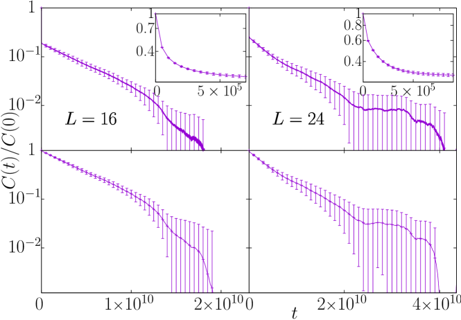
An example of the improvement obtained in the computation of the autocorrelation function is shown in Fig. 1. As it can be inferred from Eq. (7), a major difficulty is that the amplitude for $\tau_{\mathrm{exp}}$, namely $A_{1,f}$, can be very small. Indeed, the correlation function considered in a previous work [21] (which is our piece-wise linear $f$, identifier #1 in Table 1, and $T^{*}$ set to the critical temperature), has $A_{1,f}\approx 0.1$. Instead the optimized autocorrelation function has an amplitude $A_{1,f}$ almost ten times larger.

Identifier	Function
$0$	piecewise constant
$1$	piecewise linear
$2$	piecewise quadratic
$3$	piecewise cubic
$|$	OR in couples
$\&$	AND in couples
$\wedge$	XOR in couples
$*$	Multiplication in couples

Table 1: Different choices of the function $f$ used in the Variational Method.

$L$	$0$	$1$	$2$	$3$	$|$	$\&$	$\wedge$	$*$	Total
$16$	$2032$	$5320$	$3875$	$1374$	$4$	$115$	$74$	$6$	$12800$
$24$	$1556$	$7196$	$3089$	$820$	$0$	$127$	$11$	$1$	$12800$

Table 2: Number of times the variational method has picked one of the eight choices among the functions $f$ described in the text. $L$ denotes the lattice size.

We observe in Table 2 that, for almost all samples, the variational method chooses a function $f$ depending on one system copy only. Moreover, this variational method to a great extent improves substantially the results obtained previously with a linear function and a parameter $T^{*}$ chosen at the critical temperature [21].

We can do a quantitative comparison between the here proposed variational method and the old approach. Let us histogram the ratio $\tau_{\mathrm{int,old}}/\tau_{\mathrm{int,var}}$, conditioned to the value of $\tau_{\mathrm{int,var}}$ (which is a good indicator of how chaotic a sample is). We represent the result of this study in Fig. 2 where $\tau_{\mathrm{int,old}}/\tau_{\mathrm{int,var}}$ is represented for the first and last deciles of $\tau_{\mathrm{int,var}}$. The advantages of the variational estimator are evident when one focus on decile 10 (i.e. for the most chaotic samples), where we observe a significant fraction of samples with $\tau_{\mathrm{int,old}}/\tau_{\mathrm{int,var}}<0.1$.

Figure 2: Conditional probability density function of the ratio $\tau_{\mathrm{int,old}}/\tau_{\mathrm{int,var}}$, given that $\tau_{\mathrm{int,var}}$ belongs to a given decile. We show the data for the first decile (left) and the 10th-decile (right) for $L=16$ (top) and $L=24$ (bottom).

4.2 The Finite Size Scaling Behavior of the Parallel Tempering Dynamics

In this section we study the Parallel Tempering dynamics for $L=8,12,16,24$ and $32$, and we investigate temperature chaos from a dynamical point of view. In the following we will denote the mimimal temperature allowed in a parallel tempering simulation as $T_{\mathrm{min}}$ (it was $T_{1}$ in the previous section). We will focus on the variational estimate of $\tau_{\mathrm{int,var}}$ (that we will call simply $\tau$ from now on).

An implicit assumption of our study, corroborated by the results in Sect. 4.4, is that the scaling behavior of $\tau$ is mostly decided by the value $T_{\mathrm{min}}$. Other details, such as the number of temperatures in the parallel tempering mesh, are expected to play a minor role (if kept in a reasonable range). For the comparative analysis of the dynamics we use the simulations at $T_{\mathrm{min}}\approx 0.7$ shown in Table 6. This is the lowest value of $T$ we have thermalized for all our lattice sizes. An important advantage of $T_{\mathrm{min}}\approx 0.7$ is that temperature-chaos has been already characterized at such temperatures, in the equilibrium setting [39]. Lowering $T_{\mathrm{min}}$ would increase chaos effects, which would have been good in principle, but it would have been also extremely difficult to reach thermal equilibrium. Instead, increasing $T_{\mathrm{min}}$ to approach the critical point would make the results irrelevant, because samples displaying temperature chaos would be too scarce (besides, we want to study the spin-glass phase, rather than critical effects).

For $L\leq 16$ we have $N_{T}=13$. For $L=24$ we needed to increase $N_{T}$ in order to keep constant the acceptance rate of the temperature exchange step of the parallel tempering simulation. The $L=32$ data are from Ref. [21] and have been obtained with the dedicated Janus computer [63]. The Janus simulation used heat bath dynamics, rather than Metropolis, and the Parallel Tempering there had $N_{T}=34$ and $T_{\mathrm{min}}=0.703$. In order to be sure that heat bath autocorrelation times are consistent with Metropolis times (as we would expect) we simulated with Janus ten randomly selected samples with both algorithms, finding that $\tau_{\mathrm{Metropolis}}\approx\tau_{\mathrm{heat-bath}}/3$.

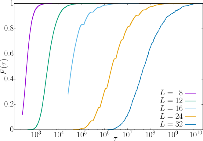
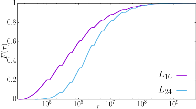
We show in Fig. 3 the cumulative distribution function of $\tau$, $F(\tau)$. The maximum slope of $F$ decreases with $L$ for the small systems, and it stabilizes between $L=24$ and $L=32$; indeed these two distributions can be approximately superposed by a simple translation. This is reminiscent of a critical slowing-down [64]

$$\tau\sim L^{z^{\mathrm{PT}}(T_{\mathrm{min}})}\,.$$ (17)

It is not obvious a priori that such a simple scaling should hold in the spin-glass phase. As a working, simplifying hypothesis we assume that the exponent $z^{\mathrm{PT}}$ only depends on the value of the lowest temperature in the parallel tempering grid, $T_{\mathrm{min}}$ (and not on the number of temperatures).

Figure 3: Empirical probability distribution of $\tau$ for $L=8,12,16,24$ and $32$. For $L=8$ and $L=12$ some of the samples have $\tau$ smaller than our minimal resolution (if $\tau<n_{\mathrm{Met}}$ we cannot compute it safely). We show only the part of the distribution function that can be safely computed.

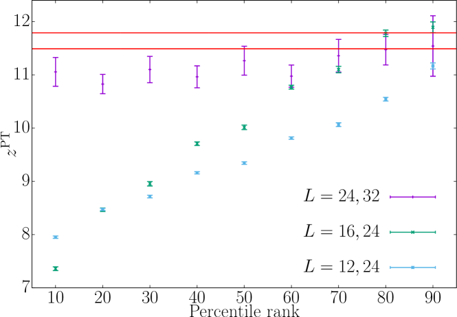
As a first test of Eq. (17) we compute an effective $z$ exponent by comparing the probability distributions for two lattice sizes $(L_{1},L_{2})$, by means of the definition

$$z^{\mathrm{PT}}(L_{1},L_{2},p)=\frac{\log(\tau(L_{1},p)/\tau(L_{2},p))}{\log(L_{1}/L_{2})}\,,$$ (18)

where $\tau(L_{i},p)$ is determined by the implicit equation $F(\tau(L_{i},p))=p/100$ where $p=1,\ldots,100$ is the so called percentile rank (i.e. $\tau(L_{i},p)$ is the $p$-th percentile of the distribution for the size $L_{i}$). We have computed $z^{\mathrm{PT}}$ for three pairs of lattice sizes, (12,24), (16,24) and (24,32) and in Fig. 4 we show the results as a function of the rank. The values for the largest pair, $(24,32)$, are independent of the rank, within statistical errors, in agreement with the ansatz. Smaller size couples give smaller estimates (in the same ball park) for low ranks, but converge to the $(24,32)$ value for high ranks (i.e. for the harder samples), and the coincidence improves and extends to smaller ranks for larger lattices. We remark that this dynamic behavior is consistent with the static findings in this temperature range [39]: for $L=8$ it is almost impossible to find samples displaying strong temperature chaos. One needs to go to systems as large as $L=24,32$ to find chaotic samples with a significant probability.

An interesting coincidence with the results of non-equilibrium simulations [65, 66, 55, 67] could have a deep meaning. Indeed in non-equilibrium conditions one finds that the spin glass correlation length $\xi$, in a lattice of size $L\gg\xi$, at temperature $T=0.7$ grows with the simulation time $t_{\mathrm{w}}$ as [66]

$$\xi(t_{\mathrm{w}})\propto t_{w}^{1/z(T)}\,,\quad z(T=0.7)=11.64(15)\,,$$ (19)

where $z(T)$ is the so-called dynamic critical exponent, that turns out to be strongly temperature dependent in the spin-glass phase $z(T)\propto T_{\mathrm{c}}/T$. Our results for the lattice pair $(24,32)$ suggest that

$$z(T=0.7)\approx z^{\mathrm{PT}}(T_{\mathrm{min}}=0.7)\,.$$ (20)

Figure 4: The effective exponent $z^{\mathrm{PT}}(L_{1},L_{2},p)$ for three different pairs of lattice sizes (12,24), (16,24) and (24,32) as a function of the percentile rank $p$. The two horizontal lines are the bounds for the off-equilibrium value $z=11.64(15)$ (see Eq. (19)). The numerical values of $z^{\mathrm{PT}}$ for the largest pair are compatible with the off-equilibrium value.

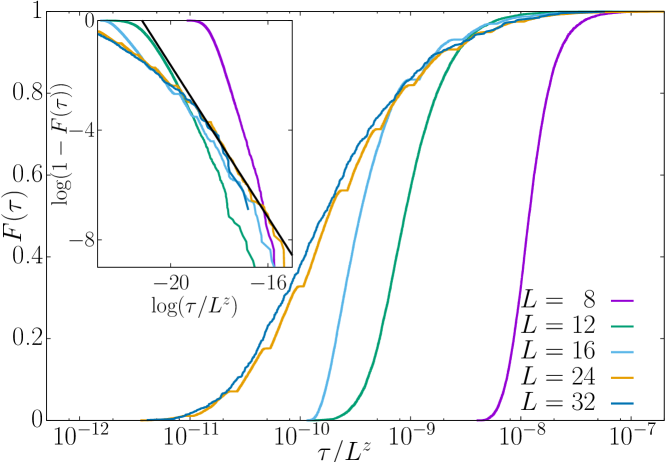
As a further test we can rescale the whole probability distribution by using Eqs. (17) and (20). This is done in figure 5 (main) that shows $F(\tau)$ as a function of $y=\tau/L^{z}$. As expected, the data for $L=24$ and $L=32$ present a nice collapse. The curve corresponding to $L=16$ collapses with them for percentile ranks higher than $80$ only and the curve corresponding to $L=12$ collapses for percentile ranks higher than $90$. This is a nice and smooth behavior. On the larger lattice sizes we reach a perfect scaling, but already on smaller lattice we see a partial scaling, that improves for increasing size. In figure 5 (inset), we show a log-log plot of $1\!-\!F(\tau)$ as a function of $\tau/L^{z}$, that emphasizes the large $\tau$ tail of the distribution. The fit presented shows that the probability density function of $\tau$ behaves, asymptotically for large $y$, like a fat tailed distribution:

$$\rho(y\equiv\tau/L^{z})\sim y^{-1-a_{1}}\,,\quad a_{1}\approx 1.38\,.$$ (21)

The distribution seems to reach its asymptotic form for $L\geq 24$. Perhaps unsurprisingly, the thermodynamic (i.e. equilibrium) effective potential that characterizes temperature chaos turns out to be also asymptotic for $L\geq 24$ [39].

Figure 5: Probability distribution function of the rescaled variable $y=\tau/L^{z}$, [$z$ is the dynamic exponent corresponding to $T_{\mathrm{min}}=0.7$, namely $z(T=0.7)=11.64(15)$]. (Inset) Plot of $\log(1-F(\tau))$ versus $\log\left(\tau/L^{z}\right)$; the straight black line is a fit to the form $a_{0}-a_{1}\log(\tau/L^{z})$ yielding $a_{0}=-29.33$ and $a_{1}=-1.38$.

In order to study how the range of temperatures in the parallel tempering affects the dynamics, we have performed an extra simulation for $L=16$. In the new simulation we take a lower minimum temperature ($T_{\mathrm{min}}=0.479$ instead of $T_{\mathrm{min}}=0.698$) increasing $N_{T}$ from $13$ to $16$ in order to keep the interval between adjacent temperatures fixed, see Table 6. Since the simulation with $N_{T}=16$ reaches a lower minimum temperature than the simulation with $N_{T}=13$ we expect to find chaos events (i.e a jam in the parallel tempering temperature flow) that the simulation with $N_{T}=13$ cannot see. In Fig. 6 we show a scatter plot of $\log(\tau_{\mathrm{int},16}/\tau_{\mathrm{int},13})$ versus $T_{d}$ for the 12800 samples ($\tau_{\mathrm{int},16}$ and $\tau_{\mathrm{int},13}$ are the autocorrelation times for $N_{T}=16$ and 13 respectively. $T_{d}$ is the temperature $T^{*}$ where the variational estimate $\tau_{\mathrm{int},f}$ reaches its maximum).

Figure 6: Scatter plot of $\log(\tau_{\mathrm{int},16}/\tau_{\mathrm{int},13})$ versus $T_{d}$. The lattice size is $L=16$, $\tau_{\mathrm{int},16}$ is the relaxation time for $N_{T}=16$ ($T_{\mathrm{min}}=0.479$), $\tau_{\mathrm{int},13}$ is the relaxation time for $N_{T}=13$ ($T_{\mathrm{min}}=0.698$), $T_{d}$ is the temperature of chaos from a dynamical point of view (defined in the variational method) of the simulation with $N_{T}=16$. Same disorder samples in the two simulations. The vertical black line represents the minimum temperature simulated in the $N_{T}=13$ simulation. (We added a small Gaussian white noise to $T_{d}$, which is a discrete variable, to avoid the cluttering of data in vertical lines).

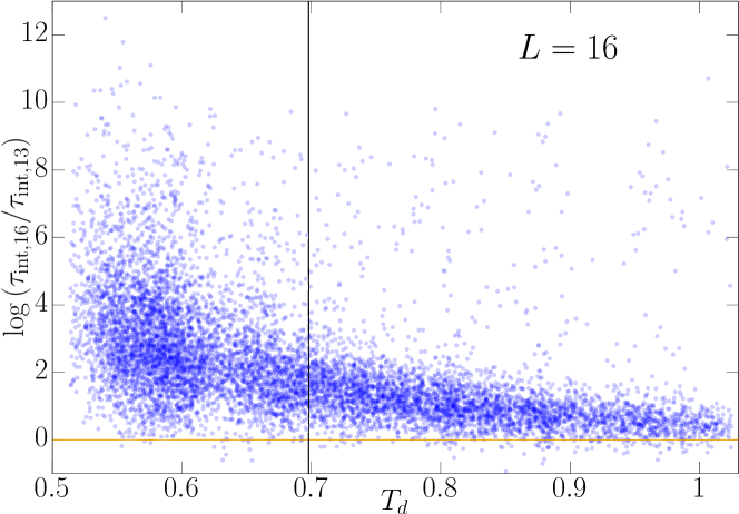
For $T_{d}>0.698$ the ratio takes values of order one for most samples, while for $T_{d}<0.698$ there is a huge number of samples with $\tau_{\mathrm{int},16}\gg\tau_{\mathrm{int},13}$, i.e. there are a lot of samples with a chaotic behavior in a temperature-range below $T_{\mathrm{min}}=0.698$.

The same idea can be analyzed from a different point of view. Imagine that we have studied with great care a given sample down to some temperature $T_{\mathrm{min}}$. Can we say something about possible chaotic effects at lower temperatures? The question is answered negatively in Fig. 7: the probability that a sample has a large $\tau_{\mathrm{int}}$ for the simulation with a lower $T_{\mathrm{min}}$ is not correlated to the value of $\tau_{\mathrm{int}}$ for the first simulation.

Figure 7: The empirical probability distribution as a function of $\tau$ for the $N_{T}=16$ simulation, conditional to the $\tau$ obtained from $N_{T}=13$ simulation belonging to a given quintile. The non-conditional probability distribution function is also shown ($L_{16}$ curve). Inset. Blowup of the top right part of the main figure. For the hard samples, the simulation with $T_{\mathrm{min}}=0.698$ conveys little or no information on the difficulty of the $T_{\mathrm{min}}=0.479$ simulation.

4.3 Statics

In the infinite volume limit, static temperature chaos is the complete rearrangement of the equilibrium configuration under any change of temperature. It has been studied numerically mostly through the disorder average of the probability density function of the overlap between the spin configurations at temperatures $T_{1}$ and $T_{2}$

$$q_{T_{1},T_{2}}=\frac{1}{V}\sum_{x}s_{x}^{T_{1}}s_{x}^{T_{2}}\,,$$ (22)

or through ratio of moments of this distribution. However, because of the size of the systems that can be currently simulated, the overlap is strongly influenced by finite size effects. It has been suggested that static temperature chaos is a rare events driven phenomena, that should be studied via the distribution of the sample-dependent chaotic parameter [39, 40]:

$$X_{T_{1},T_{2}}^{J}=\frac{\braket{q^{2}_{T_{1},T_{2}}}_{J}}{\sqrt{\braket{q^{2}_{T_{1},T_{1}}}_{J}\braket{q^{2}_{T_{2},T_{2}}}_{J}}}\,,$$ (23)

where $\braket{\cdot\cdot\cdot}_{J}$ is the thermal average within a given sample ($J$). Notice that $0<X^{J}_{T_{1},T_{2}}\lesssim 1$; $X^{J}_{T_{1},T_{2}}=1$ means that equilibrium spin configuration of the $J$ sample at temperature $T_{1}$ and temperature $T_{2}$ are indistinguishable while $X^{J}_{T_{1},T_{2}}=0$ means that the equilibrium spin configurations are completely different.

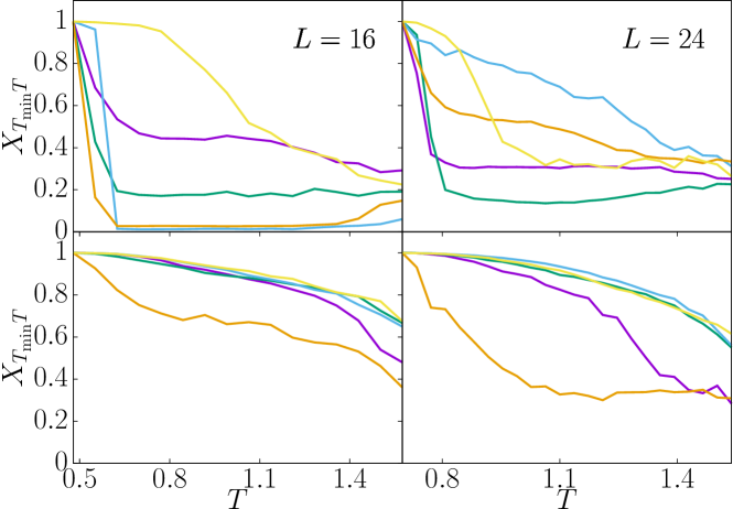
The temperature evolution of $X^{J}_{T_{1},T_{2}}$ for some selected samples is shown in Fig. 8 (in the figure $T_{1}$ is kept fixed to $T_{1}=T_{\mathrm{min}}$ while $T_{2}$ is made to vary). In some samples, we find chaotic events, namely sharp drops of $X^{J}_{T_{1},T_{2}}$ at very well defined temperatures, implying that the typical spin configurations significantly differ at the two sides of the chaotic event. It was empirically observed in Ref. [39] that chaotic events occurring at low temperatures are most harmful to the performance of parallel tempering. To quantify the effect, the chaotic integral $I$ was introduced

$$I=\int_{T_{\mathrm{min}}}^{T_{\max}}X^{J}_{T_{\mathrm{min}},T_{2}}\ \mathrm{d}T_{2}\,.$$ (24)

Note that a sharp drop of $X^{J}_{T_{\mathrm{min}},T_{2}}$ at a low $T_{2}$ will result into a very low value of the chaotic integral $I$. Furthermore, a study of the temperature behavior of the chaotic parameter leads to the conclusion that chaos events happen at low temperatures only, therefore the high temperatures introduce only noise in the estimate of $I$. In order to eliminate this noise we introduce a new integrated chaotic parameter $I_{2}$ that involves the half-lower temperatures only.

Nevertheless, there exists certain samples that exhibit a huge $\tau_{\mathrm{int}}$ and have a relative large chaotic integral, so the correlation between static and dynamics is more complicated than one could hope. Therefore, in order to improve our thermodynamic understanding of the Parallel Tempering dynamics, we need to look elsewhere. We have found it useful to consider the temperature derivative of the chaotic parameter. Indeed, it is easy to prove that:

$$\left.dX^{J}_{T_{1},T_{2}}/dT_{2}\right|_{T_{2}=T_{1}}=0\,.$$ (25)

for any temperature $T_{1}$. However, if we focus on these outlier samples, we notice that these samples present a sharp drop in $X_{T_{1},T_{2}}^{J}$ at two consecutive temperatures. This observation will motivate the definition in Eq. (26), below.

4.4 Correlations Dynamics-Static

Once we have characterized the chaos phenomena from both dynamical and static point of view, we are interested in knowing how these static and dynamics estimators are correlated.

Besides the chaos integrals $I$ and $I_{2}$, we introduce a new quantity for further use:

$$K_{i}=1-X^{J}_{T_{i},T_{i+1}}$$ (26)

After some trials, we have finally defined a last parameter:

$$I_{X}=aI_{2}-b\min_{i}\left(-\log\left(K_{i}^{2}\right)\right)-c\sum_{i}\left(-\log\left(K_{i}^{2}\right)\right)\,,$$ (27)

where the coefficients $a$, $b$ and $c$, that depends on the lattice size, are obtained through a minimization of the correlation coefficient $r$ between $I_{X}$ and $\log(\tau_{\mathrm{int}})$ ($r$ is negative, and it would be $r=-1$ if we managed to achieve a perfect understanding of our dynamical data). The values of these coefficients are given in Table 3

$L$	$a$	$b$	$c$
$16$	$0.6143$	$0.2865$	$0.1373$
$24$	$0.2963$	$0.3217$	$0.0120$

Table 3: Value of the coefficients $a$, $b$ and $c$ in Eq. 27, that maximize the correlation between $I_{X}$ and $\log(\tau_{\mathrm{int}})$.

This finding is supported by Fig. 8. We see that the most chaotic samples in terms of the integrated autocorrelation time (Fig. 8, top), present a sharp fall in the chaotic parameter. On the other hand, we can see that less chaotic samples in terms of the integrated time (Fig. 8, bottom), have a much smoother fall.

Figure 8: Plot of $X_{T_{\mathrm{min}},T}^{J}$ versus $T$ for the five most chaotic samples (top) and the five less chaotic ones (bottom): $L=16$ case (left) and $L=24$ case (right).

In Fig. 9, we confront the most representative estimator for the dynamical chaos, namely the largest integrated autocorrelation time $\tau_{\mathrm{int}}$ found in our variational study, with the static chaotic integrals $I$, $I_{2}$ and $I_{X}$. We can observe how spurious values of the original parameter $I$ (i.e. large values of $I$ associated to large $\tau_{\mathrm{int}}$) are displaced towards lower values when we use the improved parameters $I_{2}$ and $I_{X}$.

Figure 9: Scatter plot of $\log(\tau_{\mathrm{int,var}})$ versus the integrated chaotic parameter $I$. We present data for two lattice sizes and for the three definitions of the integrated chaotic parameter defined in the text ($I,I_{2}$ and $I_{X}$). The pattern of depleted horizontal bands is due to our choice of a few $l_{\mathrm{blo}}$.

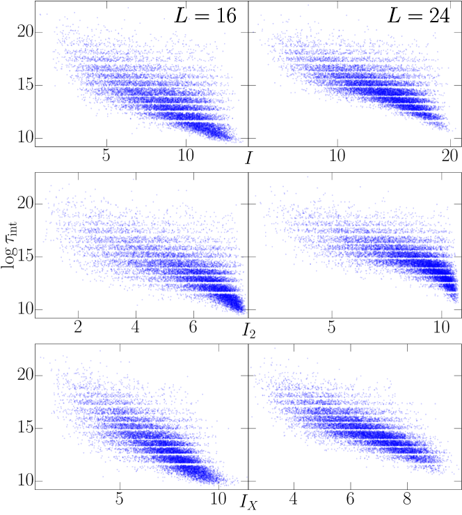
The value of the correlation coefficients are reported in Table 4. We observe a strong anti-correlation in $I_{X}$, that improves over the previous indicator of correlation $I$. [39] The improvement is less clear for $I_{2}$.

	$L$	Integral	$r$
	$16$	$I$	$-0.714\pm 0.005$
	$16$	$I_{2}$	$-0.751\pm 0.005$
	$16$	$I_{X}$	$-0.795\pm 0.004$
	$24$	$I$	$-0.725\pm 0.005$
	$24$	$I_{2}$	$-0.746\pm 0.005$
	$24$	$I_{X}$	$-0.786\pm 0.004$

Table 4: Correlation coefficients for the scatter plot of $\log(\tau_{\mathrm{int}})$ versus the integrated chaotic parameter, for each two lattice size and for the three definitions of the parameter ($I,I_{2}$ and $I_{X}$).

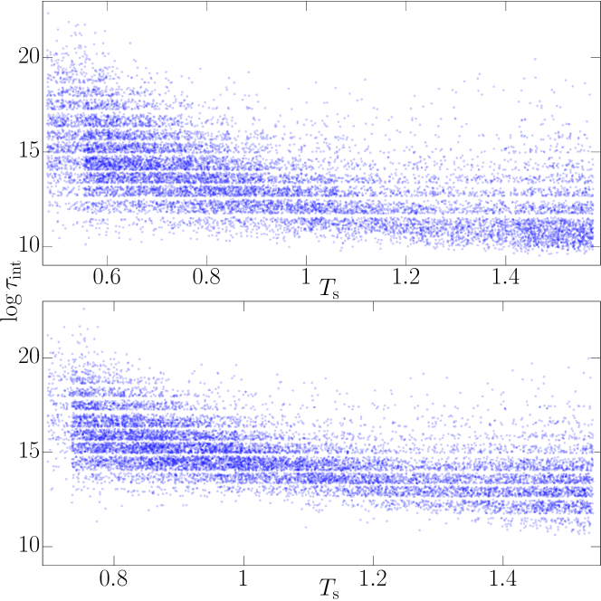
We can try to define other magnitudes (wither static or dynamical) that capture the chaos phenomenon. One possible choice is the temperature, $T_{s}$, in which $X_{T_{\mathrm{min}},T}^{J}$ presents the maximum (negative) slope. Unfortunately, we observe a weaker correlation between both estimators, $\tau$ and $T_{s}$, (see Fig. 10) and we can check it quantitatively through Table 5. Some further attempts along these lines are explored in D.

Figure 10: Scatter plot of $\log(\tau_{\mathrm{int}})$ against $T_{\mathrm{s}}$. We show $L=16$ (top) and $L=24$ (bottom). $T_{s}$ is the temperature where $X_{T_{\mathrm{min}},T}^{J}$ presents the maximum (negative) slope.

	$L$		$r$
	$16$		$-0.621\pm 0.006$
	$24$		$-0.621\pm 0.006$

Table 5: Correlation coefficients for the scatter plot of $\log(\tau_{\mathrm{int}})$ versus $T_{\mathrm{s}}$ for the two simulated lattice sizes.

5 Discussion and conclusions

We have proposed an efficient variational method to estimate the elusive exponential autocorrelation time of a Monte Carlo Markov chain, specific to the (arguably important) case of a Parallel Tempering simulation. In this variational method we have introduced three parameters (a temperature $T^{*}$, a function $f$ and a block length). We have checked that this procedure is very robust and can easily be implemented in an automatic way.

In addition, we have studied the scaling properties of the probability distribution of the autocorrelation time, obtained using the proposed variational approach. In particular we have shown that scaling holds for lattices of sizes $L\geq 24$, consistently with previous studies using effective potentials.

Moreover, we have introduced additional static chaotic indicators, and finally we have checked the statistical correlations between these static chaotic indicators and the dynamical correlation times.

6 Acknowledgments

We thank the Janus collaboration for allowing us to analyze the $L=32$ autocorrelation times from Ref. [21]. We also are grateful for allowing us to carry out a short simulation on the Janus computer, in order to establish the correspondence between the Metropolis and the Heat-bath autocorrelation times.

This project has received funding from the European Research Council (ERC) under the European Union’s Horizon 2020 research and innovation program (grant agreement No 694925). We were partially supported by MINECO (Spain) through Grant Nos. FIS2015-65078-C2, FIS2016-76359-P and by the Junta de Extremadura (Spain) through Grant No. GRU10158 (these three contracts were partially funded by FEDER). Our simulations were carried out at the BIFI supercomputing center (using the Memento and Cierzo clusters), at the TGCC supercomputing center in Bruyères-le-Châtel (using the Curie computer, under the allocation 2015-056870 made by GENCI) and at ICCAEx supercomputer center in Badajoz (grinfishpc and iccaexhpc). We thank the staff at BIFI, TGCC and ICCAEx supercomputing centers for their assistance.

Appendix A Parameters of the simulation

Whereas in numerical simulations of spin glasses the disorder samples are usually independent, the samples we use here are not fully independent. The motivations of our choice are explained in Ref. [54]. We consider cubes with $L^{3}$ spins and $3L^{3}$ couplings, divided into an inner part of $(L/2)^{3}$ spins and an outer part surrounding it. We simulate $10$ independent inner samples, and, for each inner sample, $1280$ independent outer samples. We simulate four replica (independent spin systems) for every inner and outer sample. Hence we have simulated $12800$ disorder realizations (samples) with a total of $12800\times 4$ real spin systems. The parameters of the simulation can be found in Table 6.

The thermalization criteria that have been used is as follows (as explained above these criteria applied to every sample, individually). First of all, the number of iterations in $\tau_{\mathrm{exp}}$ units ($l_{\mathrm{blo}}=1$) must be greater than $20$; as a double-check to avoid failures in the automated fitting procedure, we recomputed $\tau_{\mathrm{exp}}$ with $l_{\mathrm{blo}}=10$ (the total simulation length is also required to be longer than $20\tau_{\mathrm{exp}}^{l_{\mathrm{blo}}=10}$).

However, we had some additional safety checks to ensure that the computation of $\tau_{\mathrm{exp}}$ could be trusted. For those samples where any of the following two requirements was not met, we doubled the total simulation length and, only afterwards, we recomputed $\tau_{\mathrm{exp}}$. First, in order to make sure that every sample spends enough time at high temperatures, we require that each copy of the system in the Parallel Tempering method spends at least $35\%$ of the time in the upper half temperature region. Second, the ratio between the larger and the smaller values of $\tau_{\mathrm{int}}$, as computed for each of the four independent replica, must be less than two (for either $l_{\mathrm{blo}}=1,10,100$). This last requirement can help us to identify a lack of thermalization for those samples whose leading term in the autocorrelation function has a very small amplitude.

MUSA-MSC
$L$	$L_{\mathrm{int}}$	$N_{T}$	$T_{\mathrm{min}}$	$T_{\max}$	$N_{\mathrm{Met}}$ ($\times 10^{6}$)	$\mathrm{ps/s}$
24	12	24	0.698	1.538	500	104
16	8	16	0.479	1.575	250	107
16	8	13	0.698	1.575	250	119
16	12	13	0.698	1.575	250	119
14	12	13	0.698	1.575	500	120
12	6	13	0.698	1.575	250	119
8	4	13	0.698	1.575	250	126

MUSI-MSC
$L$	$L_{\mathrm{int}}$	$N_{T}$	$N_{\mathrm{samp}}$	$N_{\mathrm{Met,min}}$	$N_{\mathrm{Met,mean}}$	$N_{\mathrm{Met,max}}$	$\mathrm{ps/s}$
				$\times 10^{6}$	$\times 10^{6}$	$\times 10^{6}$
24	12	24	2441	1000	4262	326000	57
16	8	16	2898	500	5096	355500	304
16	8	13	338	500	543	4000	306
16	12	13	314	500	578	8000	306

Table 6: Parameters of the simulations. $L$ is the lattice size; $L_{\mathrm{int}}$ the size of the inner part of the lattice; $N_{T}$, $T_{\mathrm{min}}$ and $T_{\max}$ are the number of temperatures, the minimum and the maximum temperatures used in the Parallel Tempering method; $N_{\mathrm{Met}}$ is the number of Metropolis sweeps (at each temperature); $\mathrm{ps/spin}$ is the average CPU time per spin-flip in MUSI-MSC, using an Intel Xeon CPU E5-2680 processors; $N_{\mathrm{samp}}$ denotes the number of bad samples whose simulations had to be extended in order to thermalize and finally $N_{\mathrm{Met,min}}$, $N_{\mathrm{Met,mean}}$ and $N_{\mathrm{Met,max}}$ are the minimum, mean and maximum number of Metropolis sweeps per temperature needed to reach thermalization (bad samples). The set of temperatures used is clearly the same in the MUSI-MSC and MUSA-MSC parts of this Table. The number of Metropolis sweeps between two consecutive Parallel Tempering sweeps is always $N_{\mathrm{MpPT}}=10$. For the MUSI-MSC simulation of $L=24$ we parallelized, using Pthreads, by distributing the $N_{T}=24$ system copies among 12 CPU cores in the Intel Xeon CPU E5-2680.

Appendix B On the selection of relevant parameters of the simulation

The natural question is whether our particular choice of samples (see A) affects our results. One could imagine that the results obtained from configurations sharing the same inner part could be strongly correlated, and that with only $10$ inner parts, our statistics would be insufficient. We show in Fig 11 that this is not the case for the probability distribution of $\tau$: the probability distributions of $\tau$ for the samples sharing the same $10$ inner parts are plotted separately. they are nearly indistinguishable. The average over the outer disorder (that we can call the metastate average in analogy with Ref. [54]) reduces dramatically the fluctuations due to the inner disorder. The same conclusion holds for the chaos integral (see Fig. 12)

Figure 11: Empirical probability distribution function of $\tau$ represented for the $10$ inner samples separately. $L=16$ case (top) and $L=24$ case (bottom). Averaging over the metastate (i.e. the outer samples) with fixed inner couplings reduces strongly the fluctuations between the inner samples.

Figure 12: Empirical probability distribution function of the integrated chaotic parameter. Top We compare the distribution (labeled as ”Metastate”) obtained with our particular choice of samples with the distribution obtained from $4000$ fully independent samples (data from Janus). Bottom: Distributions obtained for the $10$ inner samples plotted separately. Averaging over the metastate (over the outer couplings) reduces strongly the fluctuations between the inner samples.

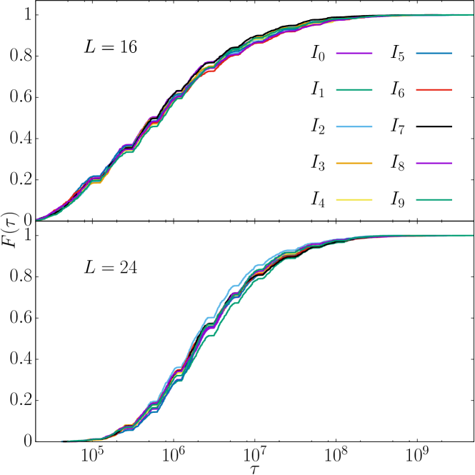
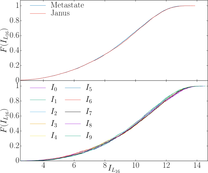
On the other hand, the selection of the minimal temperature in the Parallel Tempering could seem arbitrary, however the selection of $T_{\mathrm{min}}^{L=16}$ and $T_{\mathrm{min}}^{L=24}$ have been made carefully to assure that the most difficult samples had similar $\tau$. This is shown in the figure 13.

Figure 13: Empirical probability distribution function of $\tau$. Comparison of results for the simulations ($L=24$,$T_{\mathrm{min}}=0.698$) and ($L=16$,$T_{\mathrm{min}}=0.479$). Note that at the high-end of very difficult samples, these two simulations are similarly challenging.

Appendix C The geometry of MUSI-MSC

The geometric construction explained in Ref. [55] for $L=256$ turns out to be satisfactory as well for $L=16$, but not for $L=24$. Hence, we shall first recall the geometry that we employ for $L=16$. Afterwards, we explain the modifications that we introduced for $L=24$. Note that multispin coding is not usually employed in single-sample simulations because, in common schemes, one needs an independent random number per bit. Fortunately, this problem can be circumvented as explained in Ref. [55].

For $L=16$, the physical lattice of Cartesian coordinates $0\leq x,y,z<L$ is mapped to a super-spin lattice. Each super-spin is coded in a 256-bits computer word (of course, the 256 bits correspond to 256 physical spins which are updated in parallel). The crucial requirement is that spins which are nearest-neighbors in the physical lattice are coded into nearest-neighbors super-spins. In particular, our super-spins are placed at the nodes of a cubic lattice with the geometry of a parallelepiped of dimensions $L_{x}=L_{y}=L/8$, and $L_{z}=L/4$. The relation between physical coordinates $(x,y,z)$ and the coordinates in the super-spin lattice $(i_{x},i_{y},i_{z})$ is

$$x = b_{x}L_{x}+i_{x}\,,\ 0\leq i_{x}<L_{x}\,,\ 0\leq b_{x}<8\,,$$

$$y = b_{y}L_{y}+i_{y}\,,\ 0\leq i_{y}<L_{y}\,,\ 0\leq b_{y}<8\,,$$ (28)

$$z = b_{z}L_{z}+i_{z}\,,\ 0\leq i_{z}<L_{z}\,,\ 0\leq b_{z}<4\,.$$

In this way, exactly 256 sites in the physical lattice are given the same super-spin coordinates $(i_{x},i_{y},i_{z})$. We differentiate between them by means of the bit index:

$$i_{b}=64b_{z}+8b_{y}+b_{x}\,,\ 0\leq i_{b}\leq 255\,.$$ (29)

Since we have to simulate $N_{T}$ independent system copies in our Parallel Tempering simulation, we simply carry out successively the simulation of the $N_{T}$ systems.

The alert reader will note that the above geometric construction is very anisotropic (we start with a cube, but end-up with a parallelepiped). Fortunately, this unsightly feature can be easily fixed by noticing that the single-cubic lattice is bipartite. Indeed, the lattice splits into the even and odd sub-lattices according to the parity of $x+y+z$. The two sub-lattices contain $L^{3}/2$ sites. Furthermore, odd spins interact only with even spins and vice versa. It follows that the update ordering is irrelevant, provide that our full-lattice sweep first updates all the (say) odd sites and next all the even sites. Now, provided that $L_{x}$, $L_{y}$ and $L_{z}$ are all even, the parity of $x+y+z$ and $i_{x}+i_{y}+i_{z}$ coincide. This implies that all the spins coded in a single super-spin share the same parity, making irrelevant the super-spin lattice asymmetry. For $L=16$ one finds that $L_{x}=L_{y}=2$ and $L_{z}=4$, the three of them even numbers, and hence the above geometric construction works smoothly.

Unfortunately, for $L=24$ one has $L_{x}=L_{y}=3$ and $L_{z}=6$ which implies that the super-spin lattice cannot be split into even and odd sub-lattices. Our solution consisted in introducing logical super-spins of $512$ physical spins, that were later on coded into two computer words of 256 bits each. The geometrical correspondence was ($L_{x}=L_{y}=L_{z}=L/8$)

$$x = \tilde{b}_{x}L_{x}+j_{x}\,,\ 0\leq j_{x}<L_{x}\,,\ 0\leq\tilde{b}_{x}<8\,,$$

$$y = \tilde{b}_{y}L_{y}+j_{y}\,,\ 0\leq j_{y}<L_{y}\,,\ 0\leq\tilde{b}_{y}<8\,,$$ (30)

$$z = \tilde{b}_{z}L_{z}+j_{z}\,,\ 0\leq j_{z}<L_{z}\,,\ 0\leq\tilde{b}_{z}<8\,.$$

In this way, exactly 512 sites in the physical lattice are given the same super-spin coordinates $(j_{x},j_{y},j_{z})$. We differentiate between them by means of the bit index:

$$j_{b}=64\tilde{b}_{z}+8\tilde{b}_{y}+\tilde{b}_{x}\,,\ 0\leq i_{b}\leq 511\,.$$ (31)

Now, the crucial observation is that (because $L_{x}=L_{y}=L_{z}=3$ for $L=24$), the parity of $x+y+z$ coincides with that of $j_{x}+j_{y}+j_{z}$ if (and only if) the parity of $\tilde{b}_{x}+\tilde{b}_{y}+\tilde{b}_{z}$ is even. In other words, given super-spin coordinates $(j_{x},j_{y},j_{z})$ the 512 spins coded in the super-spin split into 256 even spins and 256 odd spins. Because same-parity spins are guaranteed to be mutually non-interacting, we decided to code the 256 bits with the same parity in the same computer word, with the corresponding bit index being the integer part of $j_{b}/2$.

However, the acceleration obtained with the MUSI-MSC was not enough for some of the worse $L=24$ samples. Hence, we decided to add an extra layer of parallelism by using Pthreads to simulate a single sample in multicore processors. Given the smallness of the super-spin lattice we found it preferable not to use concurrent threads in the simulation of a single system copies (recall that we have $N_{T}=24$ system copies in the Parallel Tempering simulation of $L=24$). Rather, we distributed the $N_{T}$ system copies along 12 CPU cores, achieving an average speed of $57$ picoseconds per spin-flip.

Appendix D Quantities not related to chaos

Figure 14: Scatter plot of $T_{d}$ versus $T_{s}$. We present the $L=16$-data (top) and the $L=24$-ones (bottom). Points are calculated with an special procedure. First, samples are classified on deciles according to $\log(\tau_{\mathrm{int}})$. The points coordinates were obtained by computing the median $T_{d}$ and the median $T_{s}$ within each decile (errors from bootstrap). The red parallel lines enclose the area of over-density that presents a higher correlation for later recount.

	$L$		$r$
	$16$		$0.348\pm 0.008$
	$24$		$0.342\pm 0.007$

Table 7: Correlation coefficients of the scatter plot of $T_{d}$ against $T_{s}$ for the simulated two lattice sizes.

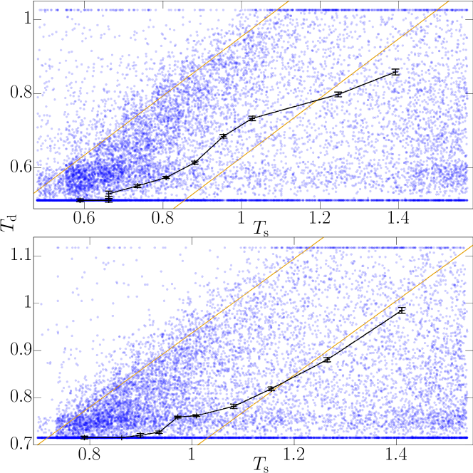
Some perfectly reasonable quantities turn out to have surprisingly little relation to temperature chaos. To illustrate this effect, we test whether or not the temperature obtained through the variational method $T_{\mathrm{d}}=\{T^{*}:\tau_{\mathrm{int}}=\tau_{\mathrm{int,var}}\}$ is correlated with the static temperature of chaos $T_{\mathrm{s}}$ (see Fig. 14).

In this case, Fig. 14 shows an over-density, however the points out of the principal density are too dispersed. For $L=16$ (top) the number of points within the lines are $8017$ ($62.63\%$ of the total) while for $L=24$ (bottom) the number of points within the lines are $7539$ ($58.90\%$ of the total). If we calculate the correlation coefficients we obtain the Table 7.

Appendix E Analyzing parallel tempering simulations

In the main text we have used theoretical tools to analyze the time series produced by a Markov chain [2] in a setting that might be unfamiliar in the context of Statistical Mechanics. In particular, in our parallel tempering simulations we have a number $N_{T}$ of independent copies (or clones) of the spin system that we want to simulate. Each clone wanders along the temperature axis, and our analysis focused solely on these temperature excursions. At first sight, the reader might be surprised by the fact that this temperature wandering may teach us something about how far the spins are from thermal equilibrium at each temperature. The purpose of this appendix is to briefly clarify the relationship between both types of degrees of freedom, namely the clone temperatures and the spins (see also Refs. [11, 68, 19, 20, 21]).

For sake of clarity, this appendix is organized in three paragraphs. A Markov Chain Monte Carlo describes a random-walk process: in E.1 we describe the phase space where our random-walk takes place. We also discuss in E.1 the stationary probability distribution (i.e. the equilibrium distribution) that our random walk is targeted to reach. In E.2 we analyze some basic facts about the dynamics of a Markov process (see for example Ref. [2] for a more detailed discussion). Finally in E.3 we consider an example that will hopefully clarify the matter further.

E.1 The phase space and the equilibrium distribution

We consider a cubic lattice of linear size $L$ with periodic boundary conditions. We define a set of $N_{T}$ temperatures, with $T_{1}<T_{2}<\cdots<T_{N_{T}}$. Our random walk moves in a discrete, very large phase space. Each state point, denoted $X$, $Y$, $Z$…hereafter, is composed of two elements.

• The spins: for each lattice site $x$ we have $N_{T}$ binary variables $s_{x}^{(\alpha)}=\pm 1$. Here, $\alpha$ is the clone index, which takes values $\alpha=1,\ldots,N_{T}$.

• The clone permutation $\pi$: $\pi$ is a permutation of $N_{T}$ symbols (there are $N_{T}!$ such permutations). The action of the permutation over the clone index $\alpha$, $\pi(\alpha)$, has a simple interpretation: it means that clone $\alpha$ is currently at temperature $T_{\pi(\alpha)}$.

In order to emphasize the composite nature of our state-point, we use the notation $X=\big{\{}\pi,\{s_{x}^{(\alpha)}\}_{\alpha=1}^{N_{T}}\big{\}}$. The state point can take $N_{T}!\,2^{N_{T}L^{3}}$ values. The position of the random walk in phase space depends on time: $X_{t}=\big{\{}\pi_{t},\{s_{x}^{(\alpha)}\}_{t,\alpha=1}^{N_{T}}\big{\}}$. The random walk has by construction the stationary distribution

$$P_{\mathrm{eq}}(X)=\frac{1}{N_{T}!}\prod_{\alpha=1}^{N_{T}}\frac{\mathrm{exp}[-H(\{s_{x}^{(\alpha)}\})/T_{\pi{(\alpha)}}]}{Z_{T_{\pi}{(\alpha)}}}\,,$$ (32)

where $H$ is the Edwards-Anderson Hamiltonian defined in Eq. (1) and $Z_{T_{\alpha}}$ is the partition function at temperature $T_{\alpha}$. One can also write it as

$$P_{\mathrm{eq}}(X)=\frac{1}{N_{T}!}\prod_{\alpha=1}^{N_{T}}\frac{\mathrm{exp}[-H(\{s_{x}^{\pi^{-1}(\alpha)}\})/T_{\alpha}]}{Z_{T_{\alpha}}}\,,$$ (33)

where $\pi^{-1}$ is the inverse permutation of $\pi$ ($\pi(\pi^{-1}(\alpha))=\alpha$ for any $\alpha$). Let us now consider the conditional probability conditioned to a given value of $\pi$. Without loss of generality we select $\pi=\mathbbm{1}$, the identity permutation, such that $\mathbbm{1}(\alpha)=\alpha$ for all $\alpha$:

$$P_{\mathrm{eq}}(X|\pi=\mathbbm{1})=\frac{\mathrm{e}^{-H(\{s_{x}^{(1)}\})/T_{1}}}{Z_{T_{1}}}\frac{\mathrm{e}^{-H(\{s_{x}^{(2)}\})/T_{2}}}{Z_{T_{2}}}\ldots\frac{\mathrm{e}^{-H(\{s_{x}^{(N_{T})}\})/T_{N_{T}}}}{Z_{T_{N_{T}}}}\,.$$ (34)

This conditional probability is a product of distributions (i.e. the spins for clones $\alpha\neq\beta$ are statistically independent, provided that $\pi$ is kept fixed), and the equilibrium probability distribution for the spins $\{s_{x}^{(\alpha)}\}$ is the Boltzmann distribution for temperature $T_{\alpha}$.

Two marginal probabilities extracted from $P_{\mathrm{eq}}(X)$ are of interest:

• Tracing-out the spin degrees-of-freedom in Eq. (32) one sees that the equilibrium probability for the clones permutation is uniform:

  $$P_{\mathrm{eq},\mathrm{marginal}}(\pi)=\frac{1}{N_{T}!}\,.$$ (35)

  Specializing to clone $\alpha$, we find $P_{\mathrm{eq}}(\pi(\alpha)=\beta)=1/N_{T}$ for any $\beta$. Checking that this has been achieved with good accuracy for all clones is one of the important tests of thermalization.

• The equilibrium probability for the spins of the clone currently at temperature $T_{\beta}$, namely $\alpha=\pi^{-1}(\beta)$, is

  $$P_{\mathrm{eq},\mathrm{marginal}}(\{s_{x}^{(\alpha)}\}|\pi(\alpha)=\beta)=\frac{\mathrm{exp}[-H(\{s_{x}^{(\alpha)}\})/T_{\beta}]}{Z_{T_{\beta}}}\,.$$ (36)

  In other words, when the random-walk equilibrates, Boltzmann equilibrium is reached at all $N_{T}$ temperatures: the spin configuration of the clone currently at temperature $T_{\beta}$ is a typical configuration of the Boltzmann distribution at such temperature.

E.2 The random walk and its correlation functions

We consider a stationary Markov process [2]. When going from time $t$ to time $t+1$ the system is updated $X_{t}\rightarrow X_{t+1}$ with a time-independent rule, that only uses as input the current state $X_{t}$. Previous states ($X_{t-1}$, $X_{t-2}$, $...$) have no influence on the decision of where to move at time $t+1$.

In our case the Markov dynamics is generated by a square matrix $G_{X,Y}$ of dimension $N_{T}!\,2^{N_{T}L^{3}}$ that meets two basic conditions, namely $G_{X,Y}\geq 0$ and $\sum_{X}G_{X,Y}=1$. In fact, $G_{X,Y}$ is a conditional probability: it is the probability for having $X_{t+1}=X$ when one knows that $X_{t}=Y$. It follows that the probability for having $X_{t=k}=X$, namely $P_{t=k}(X)$, obeys the master equation

$$P_{t=k}(X)=\sum_{Y}[G^{k}]_{X,Y}P_{t=0}(Y)\,,$$ (37)

where $G^{k}$ is the $k$-th power of the generating matrix $G$. Matrix $G$ is carefully crafted to fulfill the balance condition

$$\sum_{Y}G_{X,Y}P_{\mathrm{eq}}(Y)=P_{\mathrm{eq}}(X)\,.$$ (38)

The balance condition states that the equilibrium distribution (32) is a right-eigenvector of matrix $G$, with eigenvalue 1. When combined with the master equation, the balance condition tells us that the equilibrium distribution is a stationary distribution for our random walk.

Let us consider the spectral decomposition of the initial distribution on the $N_{T}!2^{N_{T}L^{3}}$ right-eigenvectors of matrix $G$, $Gu_{n}=\lambda_{n}u_{n}$ (ordered in such a way that $1>|\lambda_{1}|>|\lambda_{2}|>...$):

$$P_{t=0}=P_{\mathrm{eq}}+\sum_{n}c_{n}u_{n}\,.$$ (39)

The master equation implies that

$$P_{t=k}=P_{\mathrm{eq}}+\sum_{n}c_{n}\lambda_{n}^{k}u_{n}\,.$$ (40)

Hence, $P_{t=k}$ converges exponentially to $P_{\mathrm{eq}}$ and the corresponding exponential auto-correlation time is $\tau_{\mathrm{exp}}=-1/\mathrm{log}|\lambda_{1}|$.

However, the spectral analysis of the equilibrium correlation functions (see Sect. 2) is carried in terms of the left eigenvectors of matrix $G$, $\tilde{u}_{n}G=\lambda_{k}\tilde{u}_{k}$. Fortunately, for any matrix left-eigenvalues coincide with right-eigenvalues (instead, left and right eigenvectors typically differ). In fact, these are the eigenvalues appearing in Eq. (5), that we repeat here for the reader’s convenience

$$\hat{C}_{f}(t)=\sum_{n}A_{n,f}\lambda_{n}^{|t|}\,,\quad\sum_{n}A_{n,f}=1\,.$$ (41)

In particular, the constant vector $\tilde{u}_{0}$ [$\tilde{u}_{0}(X)=1$ for all states $X$] is a left eigenvector with eigenvalue 1. The generic observable $f$ considered in Eq. (41) can be decomposed as

$$f(X)=E(f)\tilde{u}_{0}(X)\ +\ \sum_{n}B_{n,f}\tilde{u}_{n}(X)\,,$$ (42)

where $E(f)$ is the equilibrium expectation value. The coefficients $A_{n,f}$ in Eq. (41) are $A_{n,f}=\tilde{B}_{n,f}/(\sum_{n^{\prime}}\tilde{B}_{n^{\prime},f})$, where $\tilde{B}_{n,f}=B_{n,f}E\big{(}\tilde{u}_{n}(X)[f(X)-E(f)]\big{)}$.

The crucial message from this analysis is that the characteristic time scales $\tau_{n}$. that one identifies by studying the correlation functions, as we did in the main text, are exactly the timescales that govern the approach to equilibrium, see Eq. (40). These characteristic times $\tau_{n}$ can be obtained from any convenient observable $f$. Whether $f$ is a spin observable, or something related to the clone permutation is immaterial. The only thing that really matters is that $A_{n=1,f}$ should be as large as possible.

E.3 An example

Just to show how deeply the spin and the temperature dynamics are intertwined, we consider here in details an example. We shall consider a typical $L=24$ sample instance (neither extremely easy, nor extremely hard: it roughly corresponds to percentile 90 of hardness, see Fig. 3).

We consider the standard parallel tempering simulation protocol from the main text: $N_{T}=24$, $T_{\mathrm{min}}=0.698$. For this particular sample one needs to run the simulation for $2\times 10^{9}$ Metropolis sweeps (for each clone) in order to meet our thermalization criteria. We also consider a truncated simulation where we only keep the lowest four temperatures: $N_{T}=4$, $T_{\mathrm{min}}=0.698$, $T_{2}=0.735$, $T_{3}=0.771$ and $T_{4}=0.808$ (all four deep in the spin-glass phase, since $T_{\mathrm{c}}=1.102(3)$ [57]). The truncated simulation is also run for $2\times 10^{9}$ Metropolis sweeps per clone.

Our expectation is that the standard simulation will equilibrate, while the truncated simulation will not. The rationale for this expectation is simple: in the standard simulation, each clone spends some $2\times 10^{9}/24\approx 8\times 10^{7}$ Monte Carlo steps at the highest temperature. Yet, the exponential auto-correlation time for the Metropolis dynamics at $T=1.6$ is about $10^{4}$ lattice sweeps [69]. Hence, the time spent by each clone at the highest temperature is long enough to effectively de-correlate the system. Instead, the highest temperature in the truncated simulation $T_{\mathrm{max,truncated}}=0.808$ lies well below $T_{\mathrm{c}}$. At such a low temperature, the Metropolis dynamics is too inefficient to decorrelate the system in only $2\times 10^{9}/4=5\times 10^{8}$ Metropolis sweeps.

Besides the temperature dynamics already considered in the main text, we shall also study here the dynamics of spin observables. Using the fact that we have already equilibrated this sample, we have selected randomly four equilibrium spin configurations at our lowest temperature $T_{\mathrm{min}}=0.698$, $\{\tau_{x,a}\}$ $a=1,2,3,4$. Then, for each clone, we compute the time-dependent overlap

$$q_{a,\alpha}(t)=\frac{1}{L^{3}}\sum_{x}\tau_{x,a}s_{x}^{(\alpha)}(t)\,.$$ (43)

We always compute the overlap with a given clone $\alpha$, irrespective its time-dependent temperature $T_{\pi_{t}(\alpha)}$.

We compute the overlaps $q_{a,\alpha}(t)$ from a set of ten new standard simulations ($N_{T}=24$), with a random start, where we measure the overlaps very often (every $5\times 10^{4}$ Metropolis sweeps). We also compute the overlaps $q_{a,\alpha}(t)$ from our new truncated simulation with $N_{T}=4$ (the truncated simulation had a random start, as well). Recall that, as we said above, the spin masks $\{\tau_{x,a}\}$ are taken from the previous sets of simulations that were discussed in the main text.

Figure 15: Top: Monte Carlo history for the overlap $q_{4}(t)$, see Eq. (43), as computed for each of the four clones in the truncated simulation (see text). Note that our simulation time is much too short to expose the symmetry $q_{4}\leftrightarrow-q_{4}$. As a consequence, we know for sure that thermal equilibrium has not been reached for the truncated simulation. Bottom: As in top panel, for the first four clones in one of our standard simulations with $N_{T}=24$ temperatures (there were 10, completely independent, standard simulations). For each clone, the overlap $q_{4}(t)$ changes sign many times along the simulation (as it is to be expected for a well equilibrated simulation). Note that, with small probability, each clone reaches a state where $|q_{4}|\sim 0.8$. These events, which are not observed for the other three overlaps $q_{a}$ $a=1,2,3$, make particularly interesting to study the dynamics of $q_{4}$.

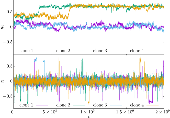
The global spin flip symmetry of the Edwards-Anderson Hamiltonian implies that the equilibrium distribution for $q_{a,\alpha}$ is symmetric under $q_{a,\alpha}\leftrightarrow-q_{a,\alpha}$. It is important to check this symmetry, since it is believed that the largest dynamical barriers are related to global spin-flips [70].

The Monte Carlo history of the time-dependent overlap with $\tau_{4}$, that we call $q_{4}$ in Fig. 15, shows very clearly that the truncated simulation is not able to reach thermal equilibrium within the time span of our simulations. The (not shown) Monte Carlo history for the other overlaps, $q_{a=1,2,3}$ are qualitatively similar. Instead, the standard simulation displays the expected symmetry under $q_{4,\alpha}\leftrightarrow-q_{4,\alpha}$. The Monte Carlo histories (in the standard simulation) for $q_{a,\alpha}$ with $a=1,2,3$ (not shown) are symmetric as well. Only $q_{4}$ uncovers a state that arises with small probability, characterized by $|q_{4}|\sim 0.8$. This feature suggests that $q_{4}$ is the most interesting overlap to look at.

Figure 16: Equilibrium time dependent correlation functions, as computed from the standard simulation with $N_{T}=24$. We consider five observables, one related to temperature (computed from the piece-wise linear function with $T^{*}=T_{3}$, see Table 1 and Sect. 4.1), and the overlaps $q_{a}$ with $a=1,2,3,4$ defined in Eq. (43). The fact that the $T$ and $q_{4}$ correlations become parallel in this semi-logarithmic scale indicates that we are safely computing the exponential auto-correlation time (which is independent of the observable). Instead, the $q_{a=1,2,3}$ correlations do not become parallel to the other curves, at least not within the range we can measure, which probably indicates that the amplitudes $A_{n=1,q_{a=1,2,3}}$, see Eq. (41), are much smaller for these observables.

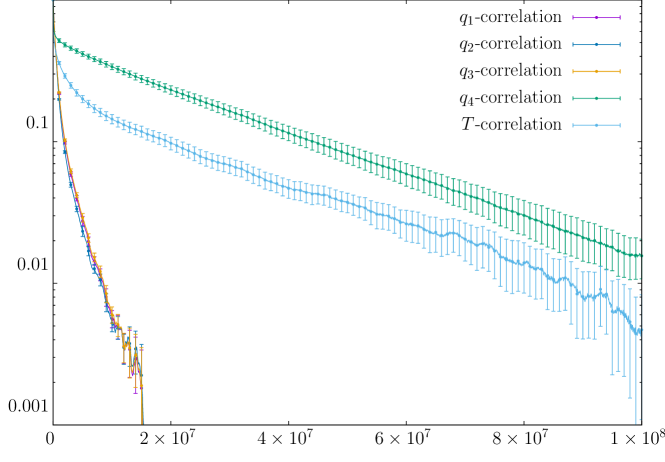
In order to make the above impressions quantitative, we show in Fig. 16 some equilibrium correlation functions, which can be computed, of course, only for the standard simulation. As it could be expected from Sect. E.2, the very same exponential auto-correlation time is computed from the temperature random walk, or from the $q_{4}$ correlation (specifically, and measuring time in Metropolis sweeps, we find $10^{-7}\tau_{\mathrm{exp}}=3.0(4)$ from $q_{4}$, while we find the fully compatible value $10^{-7}\tau_{\mathrm{exp}}=3.1(6)$ from the $T$ random-walk). One could conclude from Fig. 16 that the computation of $\tau_{\mathrm{exp}}$ is simpler by considering $q_{4}$ than by studying the temperature random walk. This is a misleading conclusion, though: we had to equilibrate the system, in the first place, in order to find the spin mask $\{\tau_{x,a=4}\}$ that defines the overlap $q_{4}$. Furthermore, the other spin masks $\{\tau_{x,a=1,2,3}\}$, turned out not to be particularly useful in the computation of the exponential auto-correlation time. It is in no way guaranteed that one can identify an interesting overlap by picking randomly a small number of equilibrated configurations.

Finally, one could consider a different question. Fig. 15 shows beyond any question that the truncated simulation does not reach equilibrium. However, there are only 4 clones in that run and one could believe that it should be not that difficult to equilibrate the clone permutation. The question is investigated in Fig. 17 by means of an occupation histogram (it is not possible to compute equilibrium correlation functions for a simulation that does equilibrate). The answer to our query is an unqualified no: the fact that the spins are out from equilibrium makes it also impossible to equilibrate the clone permutations.

Figure 17: For each of the four clones in the truncated simulation, we indicate the histogram of temperature (i.e. the number of times that $\pi_{t}(\alpha)=1$, or $\pi_{t}(\alpha)=2$, etc.). The temperature state was sampled every $5\times 10^{4}$ Metropolis sweeps (per clone). Had the simulation equilibrated, we would have expected the occupation histograms to be uniform.

References

- [1] Sokal A 1992 Quantum Fields on the Computer (Singapore: Ed. Michael Creutz, World Scientific)
- [2] Sokal A D 1997 Monte Carlo methods in statistical mechanics: Foundations and new algorithms Functional Integration: Basics and Applications (1996 Cargèse School) ed DeWitt-Morette C, Cartier P and Folacci A (N. Y.: Plenum)
- [3] Newman M E J and Barkema G T 1999 Monte Carlo Methods in Statistical Physics (Oxford: Clarendon Press)
- [4] Landau D P and Binder K 2005 A Guide to Monte Carlo Simulations in Statistical Physics 2nd ed (Cambridge: Cambridge University Press)
- [5] Mézard M, Parisi G and Virasoro M 1987 Spin-Glass Theory and Beyond (Singapore: World Scientific)
- [6] Young A P 1998 Spin Glasses and Random Fields (Singapore: World Scientific)
- [7] Cavagna A 2009 Physics Reports 476 51
- [8] Marinari E and Parisi G 1992 Europhys. Lett. 19 451
- [9] Geyer C J 1991 Markov Chain Monte Carlo Maximum Likelihood Computing Science and Statistics: Proceedings of the 23rd Symposium on the Interface ed Keramigas E M (Fairfax: Interface Foundations)
- [10] Hukushima K and Nemoto K 1996 J. Phys. Soc. Japan 65 1604
- [11] Marinari E 1998 Optimized Monte Carlo methods Advances in Computer Simulation ed Kerstész J and Kondor I (Springer-Verlag)
- [12] Sugita Y and Okamoto Y 1999 Chemical Physics Letters 314 141
- [13] Calvo F 2005 The Journal of Chemical Physics 123 124106
- [14] Earl D J and Deem M W 2005 Phys. Chem. Chem. Phys. 7(23) 3910
- [15] Brenner P, Sweet C R, VonHandorf D and Izaguirre J A 2007 The Journal of Chemical Physics 126 074103
- [16] Bittner E, Nußbaumer A and Janke W 2008 Phys. Rev. Lett. 101(13) 130603
- [17] Malakis A and Papakonstantinou T 2013 Phys. Rev. E 88(1) 013312
- [18] Sabo D, Meuwly M, Freeman D L and Doll J D 2008 The Journal of Chemical Physics 128 174109
- [19] Katzgraber H G, Trebst S, Huse D A and Troyer M 2006 Journal of Statistical Mechanics: Theory and Experiment 2006 P03018
- [20] Fernandez L A, Martín-Mayor V, Perez-Gaviro S, Tarancon A and Young A P 2009 Phys. Rev. B 80 024422
- [21] Alvarez Baños R, Cruz A, Fernandez L A, Gil-Narvion J M, Gordillo-Guerrero A, Guidetti M, Maiorano A, Mantovani F, Marinari E, Martín-Mayor V, Monforte-Garcia J, Muñoz Sudupe A, Navarro D, Parisi G, Perez-Gaviro S, Ruiz-Lorenzo J J, Schifano S F, Seoane B, Tarancon A, Tripiccione R and Yllanes D (Janus Collaboration) 2010 J. Stat. Mech. 2010 P06026
- [22] Barahona F 1982 Journal of Physics A: Mathematical and General 15 3241
- [23] Edwards S F and Anderson P W 1975 Journal of Physics F: Metal Physics F 5 965
- [24] Edwards S F and Anderson P W 1976 J. Phys. F 6 1927
- [25] McKay S R, Berker A N and Kirkpatrick S 1982 Phys. Rev. Lett. 48(11) 767
- [26] Bray A J and Moore M A 1987 Phys. Rev. Lett. 58(1) 57
- [27] Banavar J R and Bray A J 1987 Phys. Rev. B 35 8888
- [28] Kondor I 1989 J. Phys. A 22 L163
- [29] Kondor I and Végsö 1993 J. Phys. A 26 L641
- [30] Billoire A and Marinari E 2000 J. Phys. A 33 L265
- [31] Rizzo T 2001 J. Phys. A 34 5531
- [32] Mulet R, Pagnani A and Parisi G 2001 Phys. Rev. B 63 184438
- [33] Billoire A and Marinari E 2002 Europhys. Lett. 60 775
- [34] Krzakala F and Martin O C 2002 Eur. Phys. J. B 28 199
- [35] Rizzo T and Crisanti A 2003 Phys. Rev. Lett. 90(13) 137201
- [36] Sasaki M, Hukushima K, Yoshino H and Takayama H 2005 Phys. Rev. Lett. 95 267203
- [37] Katzgraber H G and Krzakala F 2007 Phys. Rev. Lett. 98 017201
- [38] Parisi G and Rizzo T 2010 Journal of Physics A: Mathematical and Theoretical 43 235003
- [39] Fernandez L A, Martín-Mayor V, Parisi G and Seoane B 2013 EPL 103 67003
- [40] Billoire A 2014 J. Stat. Mech. 2014 P04016
- [41] Wang W, Machta J and Katzgraber H G 2015 Phys. Rev. B 92(9) 094410
- [42] Fernández L A, Marinari E, Martín-Mayor V, Parisi G and Yllanes D 2016 Journal of Statistical Mechanics: Theory and Experiment 2016 123301
- [43] Martín-Mayor V and Hen I 2015 Scientific Reports 5 15324
- [44] Jonason K, Vincent E, Hammann J, Bouchaud J P and Nordblad P 1998 Phys. Rev. Lett. 81(15) 3243
- [45] Bellon L, Ciliberto S and Laroche C 2000 Europhys. Lett. 51 551
- [46] Vincent E, Depuis V, Alba M, Hammann J and Bouchaud J P 2000 Europhys. Lett. 50 674
- [47] Bouchaud J P, Doussineau P, de Lacerda-Arôso T and Levelut A 2001 Eur. Phys. J. B 21 335
- [48] Ozon F, Narita T, Knaebel A, Debrégeas Hébraud P and Munch J P 2003 Phys. Rev. E 68 032401
- [49] Yardimci H and Leheny R L 2003 Europhys. Lett. 62 203
- [50] Mueller V and Shchur Y 2004 Europhys. Lett. 65 137
- [51] Guchhait S and Orbach R L 2015 Phys. Rev. B 92(21) 214418
- [52] Katzgraber H G, Hamze F, Zhu Z, Ochoa A J and Munoz-Bauza H 2015 Phys. Rev. X 5(3) 031026
- [53] Marshall J, Martin-Mayor V and Hen I 2016 Phys. Rev. A 94(1) 012320
- [54] Billoire A, Fernandez L A, Maiorano A, Marinari E, Martin-Mayor V, Moreno-Gordo J, Parisi G, Ricci-Tersenghi F and Ruiz-Lorenzo J J 2017 Phys. Rev. Lett. 119(3) 037203
- [55] Fernández L A and Martín-Mayor V 2015 Phys. Rev. B 91(17) 174202
- [56] Manssen M and Hartmann A K 2015 Phys. Rev. B 91(17) 174433
- [57] Baity-Jesi M, Baños R A, Cruz A, Fernandez L A, Gil-Narvion J M, Gordillo-Guerrero A, Iniguez D, Maiorano A, Mantovani F, Marinari E, Martín-Mayor V, Monforte-Garcia J, Muñoz Sudupe A, Navarro D, Parisi G, Perez-Gaviro S, Pivanti M, Ricci-Tersenghi F, Ruiz-Lorenzo J J, Schifano S F, Seoane B, Tarancon A, Tripiccione R and Yllanes D (Janus Collaboration) 2013 Phys. Rev. B 88 224416
- [58] Lulli M, Bernaschi M and Parisi G 2015 Computer Physics Communications 196 290
- [59] Leuzzi L, Parisi G, Ricci-Tersenghi F and Ruiz-Lorenzo J J 2008 Phys. Rev. Lett. 101(10) 107203
- [60] Baños R A, Fernandez L A, Martin-Mayor V and Young A P 2012 Phys. Rev. B 86(13) 134416
- [61] Fernández L A, Martin-Mayor V, Parisi G and Seoane B 2010 Phys. Rev. B 81(13) 134403
- [62] Amit D J and Martín-Mayor V 2005 Field Theory, the Renormalization Group and Critical Phenomena 3rd ed (Singapore: World Scientific)
- [63] Belletti F, Guidetti M, Maiorano A, Mantovani F, Schifano S F, Tripiccione R, Cotallo M, Perez-Gaviro S, Sciretti D, Velasco J L, Cruz A, Navarro D, Tarancon A, Fernandez L A, Martín-Mayor V, Muñoz-Sudupe A, Yllanes D, Gordillo-Guerrero A, Ruiz-Lorenzo J J, Marinari E, Parisi G, Rossi M and Zanier G (Janus Collaboration) 2009 Computing in Science and Engineering 11 48
- [64] Zinn-Justin J 2005 Quantum Field Theory and Critical Phenomena 4th ed (Oxford: Clarendon Press)
- [65] Belletti F, Cotallo M, Cruz A, Fernandez L A, Gordillo-Guerrero A, Guidetti M, Maiorano A, Mantovani F, Marinari E, Martín-Mayor V, Sudupe A M, Navarro D, Parisi G, Perez-Gaviro S, Ruiz-Lorenzo J J, Schifano S F, Sciretti D, Tarancon A, Tripiccione R, Velasco J L and Yllanes D (Janus Collaboration) 2008 Phys. Rev. Lett. 101 157201
- [66] Belletti F, Cruz A, Fernandez L A, Gordillo-Guerrero A, Guidetti M, Maiorano A, Mantovani F, Marinari E, Martín-Mayor V, Monforte J, Muñoz Sudupe A, Navarro D, Parisi G, Perez-Gaviro S, Ruiz-Lorenzo J J, Schifano S F, Sciretti D, Tarancon A, Tripiccione R and Yllanes D (Janus Collaboration) 2009 J. Stat. Phys. 135 1121
- [67] Baity-Jesi M, Calore E, Cruz A, Fernandez L A, Gil-Narvión J M, Gordillo-Guerrero A, Iñiguez D, Maiorano A, Marinari E, Martin-Mayor V, Monforte-Garcia J, Muñoz Sudupe A, Navarro D, Parisi G, Perez-Gaviro S, Ricci-Tersenghi F, Ruiz-Lorenzo J J, Schifano S F, Seoane B, Tarancón A, Tripiccione R and Yllanes D 2017 Proceedings of the National Academy of Sciences 114 1838
- [68] Marinari E, Parisi G and Ruiz-Lorenzo J J 1998 Numerical Simulations of Spin Glass Systems Spin glasses and random fields ed Young A P (Singapore: World Scientific)
- [69] Ogielski A T 1985 Phys. Rev. B 32 7384
- [70] Billoire A and Marinari E 2001 Journal of Physics A: Mathematical and General 34 L727