propositionprop \equalenvcorollarycoro \equalenvdefinitiondefi \equalenvremarkrema \alttitleForme limite et fluctuations de hauteur pour les couplages parfaits aléatoires des graphes carrés-hexagones \altkeywordsdimères, couplage parfait, forme limite, champ libre gaussien, fonction de Schur
Limit shape and height fluctuations of random perfect matchings on square-hexagon lattices
Abstract.
We study perfect matchings on the contracting square-hexagon lattice, constructed row by row from a row of either the square grid or the hexagonal lattice. Given periodic weights to edges, we consider the probabilities of dimers proportional to the product of edge weights. We show that the partition function equals a Schur function of the edge weights. We then prove the Law of Large Numbers (limit shape) and the Central Limit Theorem (convergence to the Gaussian free field) for the corresponding height functions. We also show that certain type of dimers near the turning corner converge in distribution to the eigenvalues of Gaussian Unitary Ensemble, and that in the scaling limit when each segment of the bottom boundary grows linearly with respect to the dimension of the graph, the frozen boundary is a cloud curve with multiple tangent points (depending on the period) along each horizontal boundary segment.
Key words and phrases:
dimer, perfect matching, limit shape, Gaussian free field, Schur function1991 Mathematics Subject Classification:
82B20, 05E05, 74A50 ,60B20Nous étudions les couplages parfaits de graphes, construits en prenant, pour chaque ligne, une ligne soir du réseau carré, soit du réseau hexagonal. Étant donnés des poids sur les arêtes avec une période , la fonction de partition est une fonction de Schur dépendant des poids. Nous obtenons dans la limite des grands systèmes une loi des grands nombres (forme limite) et un théorème central limite (convergence vers le champ libre) pour la fonction de hauteur associée. La distribution de certains dimères près du point de contact au bord converge vers celle des valeurs propres de l’ensemble unitaire gaussien. De plus, dans la limite d’échelle de systèmes pour lesquels chaque segment du bord croît linéairement avec la taille du graphe, le bord de la zone gelée est une courbe nuage avec des points de contact sur chaque segment du bord inférieur dont le nombre dépend de la période.
1. Introduction
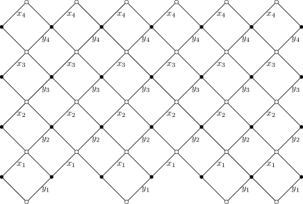
A perfect matching, or a dimer configuration, is a subset of edges of a graph such that each vertex is incident to exactly one edge. We study the asymptotic behavior of periodically weighted random perfect matchings on a class of domains called the contracting square hexagon lattice. Each row of the lattice is either obtained from a row of a square grid or that of a hexagon lattice; see Figure 2.6 for an example. On such a graph we shall assign edge weights, satisfying the condition that the edge weights are invariant under under horizontal translations, while changing row by row. We define a probability measure for dimer configurations on such a graph to be proportional to the product of edge weights.
When all the edge weights are 1, the underlying probability measure is the uniform measure. The uniform perfect matchings on a square grid or a hexagonal lattice have been studied extensively in the past few decades; see [42, 16, 15] for recent results about uniform perfect matchings on the hexagonal lattice, and [8] for recent results about uniform perfect matchings on the square grid. These results are obtained by applying and re-developing the recent techniques developed to study the Schur processes; see [38, 40, 1, 2, 7, 6]. Dimer model on a more general graph, called the rail-yard graph, may also be studied by techniques of Schur processes; see [5].
Among the problems concerning the asymptotic behavior of perfect matchings on larger and larger graphs, two of them are of special interest: the Law of Large Numbers and the Central Limit Theorem. More precisely, when the underlying finite graphs on which the dimer configurations are defined become larger and larger whose rescaled version approximate a certain domain in the plane, the rescaled height functions (which is a random function defined on faces of the graph associated to each random perfect matching) are expected to converge to a deterministic function (limit shape); and the non-rescaled height function is expected to have Gaussian fluctuation. The limit shape behavior was first observed from the arctic circle phenomenon for dimer models on large Aztec diamond (which is a finite subgraph of the square grid with certain boundary conditions); see [23, 21]. In each component outside the inscribed the circle, with probability exponentially close to 1, all the present edges of the dimer configuration are along the same direction. This is called the frozen region. Inside the circle, the probability that an edge of any certain direction appears in the dimer configuration is non-degenerate and lies in the open interval ; this is called the liquid region. The limit shape of non-uniform dimer models on square grids, with more general boundary conditions, was studied in [10], and the technique may be generalized to obtain a variational principle, limit shape, and equation of frozen boundary for dimer models on general periodic bipartite graphs; see [27]. The Aztec diamond with period was studied in [9], with period was studied in [11].
A square-hexagon lattice may be constructed row by row from either a row of a square grid or a row of a hexagonal lattice. In this paper, we assign positive weights to edges of the square-hexagon lattice in such a way that the edge weights change row by row with a fixed finite period. We then consider a special finite subgraph of the square-hexagon lattice, called a contracting square-hexagon lattice. With the help of the branching formula for the Schur function, we then show that the partition function of dimer configurations on a contracting square hexagon lattice, can be computed by a Schur function depending on edge weights.
Note that Markov chains for sampling those random dimer configurations on finite square-hexagon lattices with certain boundary conditions (i.e. random tilings of tower graphs) were studied in [4].
We then study the limit shape of the dimer configurations when the mesh size of the graph goes to zero, and show that the height function converges a deterministic function with an explicit formula. We then find the equation of the frozen boundary, and show that the frozen boundary is again a cloud curve (similar results was obtained in [27] for the hexagonal lattice, and obtained in [8] for the square grid), whose number of tangent points to the bottom boundary depend not only on the number of segments with distinct boundary conditions on the bottom boundary, but also on the size of the period of edge weights. In particular, given our assignments of edge weights, the liquid region is a simply-connected domain, i.e. there are no “floating bubbles” in the liquid region. We then study the fluctuations of non-rescaled height function, and show that after a homeomorphism from the liquid region to the upper half plane, the law of non-rescaled height fluctuations are given in the limit by the Gaussian free field. This extends the framework in which such a result is available for non-flat boundary conditions. See [3, 12] for the first results of this type, and [13] for another method to show that a large class of models have this kind of fluctuations. We also study the distribution of present edges joining a row with odd index to a row with even index above it, and show that near the top boundary, these edges have the same distribution as the eigenvalues of a GUE random matrix, which was established in [39] for plane partitions and in [22] for the Aztec diamond. In [30, 29], the case when the periodic edge weights decay polynomially with respect to the size of the graph is investigated, the liquid region is proved to split to finitely many disconnected components, and the height fluctuation in each component of the liquid region is proved to be an independent Gaussian free field in the scaling limit.
The organization of the paper is as follows. In Section 2, we define the contracting square-hexagon lattice and prove the formula to compute the partition function of dimer configurations on such a lattice via Schur functions depending on edge weights. In Section 3, we prove an explicit formula for the limit of the rescaled height function. In Section 4, we prove an explicit formula for the density of the limit counting measure associated to the dimer configurations on each row of the contracting square-hexagon lattice, and define the frozen region to be the region whenever the density is 0 or 1. In Section 5, we prove an explicit formula for the frozen boundary (the boundary of the frozen region) and show that the frozen boundary a cloud curve. In Section 6, we show that the distribution of present edges joining an row with odd index to a row with even index above it near the top boundary is the same as that of eigenvalues of a GUE random matrix. In Section 7, we show that the fluctuation of the non-rescaled height function is a homeomorphism of the Gaussian free field in the upper half plane. In Section 8, we give simulations of the distribution of dimer models on the contracting square-hexagon lattice, and draw pictures of the limit shape.
2. Combinatorics
In this section, we define the contracting square-hexagon lattice on which we shall study the perfect matching, or the dimer model. By an explicit bijection between perfect matchings on the contracting square-hexagon lattice and sequences of certain Young diagrams, we express the probability measure on perfect matchings, in which the probability of each configuration is proportional to product of edge weights, in terms of Schur functions. As a result, the partition function of dimer configurations on such contracting square-hexagon lattice can also be expressed in term of Schur functions. This extends known results for the dimer model on the square grid [8] and hexagonal lattice [42, 6], where the underlying measure is uniform or a -deformation of the uniform measure.
2.1. Square-hexagon Lattices
Consider a doubly-infinite binary sequence indexed by integers .
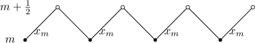
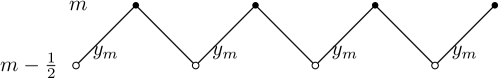
The whole-plane square-hexagon lattice associated with the sequence , is a bipartite plane graph defined as follows. Each vertex of is either black or white, and we identify the vertices with points on the plane. Its vertex set is a subset of . For , the vertices with ordinate correspond to the th row of the graph. Vertices on even rows (for integer) are colored in black. Vertices on odd rows (for half integer) are colored in white.
-
•
each black vertex on the th row is adjacent to two white vertices in the th row; and
-
•
if , each white vertex on the th row is adjacent to exactly one black vertex in the th row; if , each white vertex on the th row is adjacent to two black vertices in the th row.
See Figure 2.1. Such a graph is also related to the rail-yard graph; see [5].

We shall assign edge weights to the whole-plane square-hexagon lattice as follows.
Assumption 1.
For , we assign weight to each NE-SW edge joining the th row to the th row of . We assign weight to each NE-SW edge joining the th row to the th row of , if such an edge exists. We assign weight to all the other edges.
It is straightforward to check the following lemma describing the faces of a whole-plane square-hexagon lattice.
Lemma 2.1.
Each face of is either a square (degree-4 face) or a hexagon (degree-6 face). Let be a positive integer.
-
(1)
There exists a degree-6 face including both black vertices in the th row and black vertices in the th row if and only if .
-
(2)
There exists a degree-4 face including both black vertices in the th row and black vertices in the th row if and only if .
A contracting square-hexagon lattice is built from a whole-plane square-hexagon lattice as follows:
Definition 2.2.
Let . Let be an -tuple of positive integers, such that . Set . The contracting square-hexagon lattice is a subgraph of built of or rows. We shall now enumerate the rows of inductively, starting from the bottom as follows:
-
•
The first row consists of vertices with and . We call this row the boundary row of .
-
•
When , for , the th row consists of vertices with and incident to at least one vertex in the row of the whole-plane square-hexagon lattice lying between the leftmost vertex and rightmost vertex of the th row of
-
•
When , for , the th row consists of vertices with and incident to two vertices in the th row of of .
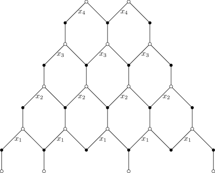
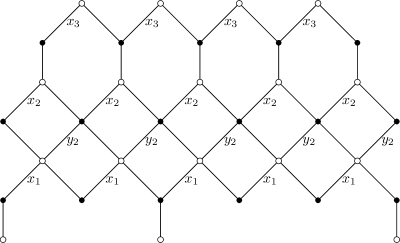
The transition from an odd row to the next even row in a contracting square-hexagon lattice can be of two kinds depending on whether vertices are connected to one or two vertices of the row above them. See Figures 2.4, 2.5, and 2.6 for examples of contracting square-hexagon lattices.
Definition 2.3.
Let (resp. ) be the set of indices such that vertices of the th row are connected to one vertex (resp. two vertices) of the th row. In terms of the sequence ,
The sets and form a partition of , and we have .
2.2. Perfect Matching
Definition 2.4.
A dimer configuration, or a perfect matching of a contracting square-hexagon lattice is a set of edges , such that each vertex of belongs to a unique edge in .
The set of perfect matchings of is denoted by .
Definition 2.5.
Let be a perfect matching of . We call an edge a -edge if (i.e. if its higher extremity is black) and we call it a -edge otherwise. In other words, the edges going upwards starting from an odd row are -edges and those ones starting from an even row are -edges. We also call the corresponding vertices- and -vertices and -vertices accordingly.
Lemma 2.6.
Let be a perfect matching of . For each , the number of -edges joining the th row and the th row is one more than the number of edges joining the th row and the th row.
Proof 2.7.
For , let be the number of vertices in the th row of . From the construction of in Definition 2.2, we have
| (2.1) |
Let be the number of -edges joining the th row and th row. Then there exists -edges joining the th row to the th row. Hence there are -edges joining the th row and th row. Then the lemma follows from (2.1).
Example 2.8.
- (1)
- (2)
2.3. Partitions and Young Diagrams
Following [8], we will use signatures to encode the perfect matchings of of the contracting square-hexagons.
Definition 2.9.
A signature of length is a sequence of nonincreasing integers . Each is a part of the signature . The length of the signature is denoted by . We say that is non-negative if . The size of a non-negative signature is
denotes the set of signatures of length , and is the subset of non-negative signatures.
To the boundary row of a contracting square-hexagon lattice is naturally associated a non-negative signature of length by:
Non-negative signatures are the convenient objects to talk about integer partitions with a given number of zero parts. Most of the objects constructed from partitions are available for non-negative signatures, in particular Young diagrams, and interlacement relations which we recall now.
A graphic way to represent a non-negative signature is through its Young diagram , a collection of boxes arranged on non-increasing rows aligned on the left: with boxes on the first row, boxes on the second row,… boxes on the th row. Some rows may be empty if the corresponding is equal to 0. The correspondence between non-negative signatures of length and Young diagrams with (possibly empty) rows is a bijection.
If all the parts of a non-negative signature are equal (say parts equal to ), the Young diagram has a rectangular shape. We then say that is rectangular, and note , and for its Young diagram.
Young diagrams included in are those corresponding to non-negative signatures of length and parts bounded by .
Definition 2.10.
Let be two Young diagrams. We say that differ by a horizontal strip if the collection of boxes in contains at most one box in every column. We say that they differ by a vertical strip if contains at most one box in every row.
We say that two non-negative signatures and interlace, and write if differ by a horizontal strip. We say they co-interlace and write if differ by a vertical strip.
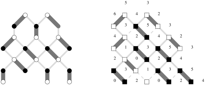
Another way to graphically represent signatures is to use Maya diagrams, which usually represent a collection of white and black particles (here squares , ) on the 1-dimensional lattice . For our purposes, since we will work with non-negative signatures with Young diagram included in a rectangle of a given size, we will need finite version of Maya diagrams, defined below.
Definition 2.11.
A finite Maya diagram of length is an element of . The origin of the Maya diagram is a position between two successive elements of the sequence, such that the number of elements on the left (resp. on the right) of this position is equal to the number of (resp. ) particles.
Non-negative signatures of length with parts bounded by corresponds bijectively to finite Maya diagrams of length and exactly black particles, by the following coding of the non trivial part of the boundary of seen as a lattice path of length connecting two opposite corners of . A vertical step corresponds to a and a horizontal step corresponds to a . See Figure 2.2.
This way, the signature of length with all parts equal to (resp. equal to ) corresponds to the Maya diagram where the black particles are on the left (resp. on the right) of the white particles.

We shall associate to each perfect matching in a sequence of non-negative signatures, one for each row of the graph.
Construction 1.
Let . Assume that the th row of has V-vertices and -vertices. Then we first associate a finite Maya diagram of length with black particles: every -vertex (resp. -vertex) is mapped to a white (resp. black) particle. This Maya diagram corresponds then to a Young diagram of a non-negative signature of length and parts bounded by , which in turn has a Young diagram fitting in a rectangle.
Note that to perform this construction for the boundary row (i.e. ), vertices with coordinates between and , which are not present in the graph are considered a (virtual) -vertices, and should be taken into account to compute and .
The encoding of dimer configurations of finite contracting square-hexagon graphs with Maya diagrams allows then for a bijective correspondence with sequences of interlaces signatures. More precisely:
Theorem 2.12 ([8] Theorem 2.9, [5]).
For given , , let be the signature associated to . Then the construction 1 defines a bijection between the set of perfect matchings and the set of sequences of non-negative signatures
where the signatures satisfy the following properties:
-
•
All the parts of are equal to 0;
-
•
The signature is equal to ;
-
•
The signatures satisfy the following (co)interlacement relations:
Moreover, if , then .
Remark 2.13.
The interlacing relations have the following implications on the signatures and their Young diagrams:
-
•
for all , ;
-
•
for all , parts of (resp. ) are all bounded by (resp. ).
where
is the number of odd rows below with ordinate less than , where vertices are connected to a single vertex of the row above them.
The following lemma relates the size of the signatures associated to rows of the graph with the number of NE-SW dimers connecting these rows:
Lemma 2.14.
-
Let .
-
(1)
If in the th row of , the dimer configuration is given by the signature ; and in the th row, the dimer configuration is given by the signature , then the number of present NE-SW edges joining the th row to the th row is .
-
(2)
Assume that each vertex in the th row of is adjacent to two vertices in the th row. If in the th row of , the dimer configuration is given by the signature ; and in the th row, the dimer configuration is given by the signature , then the number of present NE-SW edges joining the th row to the th row is .
Proof 2.15.
Edges present in a dimer configuration between rows and are -edges, connecting -vertices which in terms of Maya diagram are -particles.
Let (resp. ) be Maya diagrams corresponding to and . Note that (resp. ) has exactly (resp. ) boxes to the left of its origin, and both and have the same number of boxes to the right or their origins. This follows from the fact that (resp. ) has (resp. ) black squares, while both and have the same number of white squares; see Definition 2.11. If we look at the and with their origin aligned, the presence of a NE-SW edge corresponds to a -particle in jumping to the right by one step in (whereas a NW-SE edge would correspond to a -particle staying at the same place in both and ; see Figure 2.3.
The number of NE-SW edges between these two rows is thus the total displacement of -particles. Since in a Maya diagram, moving a -particle to the right corresponds to removing a box in the Young diagram, thus decreasing the size of the partition by 1, it follows that the total displacement of the -particles is equal to .
The second part is proved analogously.

A simple and direct consequence of Lemma 2.14 is the following:
Corollary 2.16.
The total number of NE-SW edges in a perfect matching of is equal to , the size of the non-negative signature corresponding to the boundary row .
2.4. Schur Functions and Partition Function of Perfect Matchings
Recall that the partition function of the dimer model of a finite graph with edge weights is given by
where is the set of all perfect matchings of . The Boltzmann dimer probability measure on induced by the weights is thus defined by declaring that probability of a perfect matching is equal to
In this section, we prove a formula which express the partition function of perfect matchings on a contracting square-hexagon lattice as a Schur function depending on the boundary configuration and the edge weights.
Definition 2.17.
Let . The rational Schur function associated to is the homogeneous symmetric function of degree in variables defined by:
Let be two non-negative signature of length . It is well-known that Schur functions form a basis for the algebra of symmetric functions. Let . We define as in [8] the coefficients and as follows:
| (2.2) |
and
| (2.3) |
By the branching formula for Schur polynomials, and the same argument as [8, Lemma 2.12] we have the following identities
| (2.4) | ||||
| (2.5) |
from which we deduce that the following holds:
For , define
| (2.6) |
and for , define
| (2.7) |
By homogeneity of the Schur functions, for each , and , we have
| (2.8) |
For , define
| (2.9) |
Recall that , as defined in Theorem 2.12, is the set of all the sequences of partitions in bijection with the set , which consists of all the perfect matchings on the contracting square-hexagon lattice with bottom boundary condition and structures on rows given by . We now define a probability measure on as follows:
| (2.10) |
The following proposition connects this measure with the Boltzmann measure on dimers configurations of the associated contracting square-hexagon graph:
Proposition 2.18.
The bijection described in Theorem 2.12 transports the probability measure (2.10) on to a Boltzmann dimer measure on the perfect matchings of , with the following weights
-
•
each NE-SW edge joining the th row to the th row has weight ; and
-
•
each NE-SW edge joining the th row to the th row has weight , if such an edge exists;
-
•
All the other edges have weight 1.
Moreover, the dimer partition function on for these weights is given by
where is the -tuple corresponding to the boundary row of , and is defined as in (2.9).
2.5. Examples
In this section, we provide a few examples of contracting square-hexagon lattices, compute the partition functions of dimer configurations on these graphs explicitly, and verify that these partition functions are equal to the formula given by Proposition 2.18.
2.5.1. Square Grid
Consider perfect matchings on a square grid with edge weights assigned as in the Figure 2.4.
Corollary 2.20.
Let be a contracting square grid, with edge weights on NE-SW edges; for all ; and is an -tuple of integers. Then the partition function for perfect matchings on is given by
where is the -tuple corresponding to the boundary row of , and is defined as in (2.9).
Proof 2.21.
The case when all and are 1 is the one covered by [8].
2.5.2. Hexagon Lattice
Corollary 2.22.
Let be a contracting hexagonal lattice such that for all and is an -tuple of integers, with edge weights on NE-SW edges. Then the partition function for perfect matchings on is given by
where is the -tuple corresponding to the boundary row of , and is defined as in (2.9).
Proof 2.23.
The case when all the weights are equal to 1 is the context of [42], although the results there were obtained through a -deformation of the measure by setting and taking the limit .
2.5.3. A Square-Hexagon Lattice
Example 2.24.
The partition function of dimer configurations on a square-hexagon lattice as illustrated in Figure 2.6 is
| (2.12) |
Indeed, in the graph shown in Figure 2.6, we have and the boundary signature is . Then the partition function can be computed by applying Proposition 2.18. More precisely
Expanding , we obtain exactly (2.12).
For this case, as well as the previous cases, an alternative way to derive the partition function would be to apply Kasteleyn–Percus theory [24, 41] and write it as the determinant of a sign twisted, weighted, bipartite adjacency matrix of the graph, and get the same polynomials. But for this class of graphs, the machinery of symmetric functions gives a shorter derivation of the partition function.
2.6. Convergence of the free energy
We state now a result about the asymptotic behavior of the partition function Z of the dimer model on contracting square-hexagon graphs (defined in Proposition 2.18), subject to some regularity for the sequence of signatures describing the boundary of the graph. This partition function then grows exponentially with , where is the size of the graph, and the exponential growth rate
is called the free energy.
Let us introduce first some definition to state the hypotheses for the convergence result:
Let be a non-negative signature. We define the counting measure corresponding to as follows:
Let be a probability measure on the set of all signatures. The push-forward of with respect to the map defines a random probability measure on denoted by .
One natural setting for which one can prove that the free energy exists is when the corresponding sequence of signatures describing the boundary of our sequence of contracting square-hexagon graphs is regular [16], in the following sense:
Definition 2.25 ([16]).
A sequence of signatures is called regular, if there exists a piecewise continuous function and a constant such that
Since the renormalized logarithm of the factors have a simple limit, the existence and the value of the free energy is determined by the existence of the logarithm of the renormalized Schur function.
For any positive integer , let .
Proposition 2.26 (Existence of the normalized free energy in the periodic case).
Suppose that the following two conditions hold:
-
•
is a regular sequence of signatures,
-
•
as , converges weakly to a probability measure on .
Then:
-
(1)
For each , .
-
(2)
For any , and any sequence converging to , the limit
(2.13) exists, and depends only on the limit . In particular,
(2.14)
Proof 2.27.
By Corollary 2.22, is the total number of dimer configurations on a contracting hexagonal lattice, in which the boundary configuration is given by . Since there exists at least one dimer configuration on each such lattice, we obtain the first part.
The existence of the limit is a consequence of the successive application of two lemmas stated below: first Lemma 2.28 expressing the Schur function as a matrix integral, then Lemma 2.29 about limit of normalized logarithms of these integrals.
The convergence condition (2) implies that the empirical measures
converge to the same measure. Thus by Lemma 2.29, the renormalized logarithms of matrix integrals, and hence Schur functions, converge and have the same limit.
Here are the two lemmas needed to conclude the proof of the previous proposition. The first one represents the Schur function as a matrix integral over the unitary group, the so-called Harish–Chandra–Itzykson–Zuber integral:
Lemma 2.28 ([19, 20]).
Let be a non-negative signature, and let be an diagonal matrix given by
Let , and let be an diagonal matrix given by
Then,
| (2.15) |
where is the Haar probability measure on the unitary group .
Note that Lemma 2.28 was originally proved when is a Hermitian matrix with eigenvalues , hence . Since the right hand side of (2.15) depends only on the eigenvalues of when is a Hermitian matrix, the identity (2.15) is then true for with complex entries as well since both the left hand side and the right hand side in (2.15) are entire functions in .
The second lemma is about the convergence of the normalized logarithms of these integrals:
Lemma 2.29 ([18], Theorem 1.1).
For an Hermitian matrix with eigenvalues , we denote by
the spectral measure for . Let , be two sequences of diagonal, real-entry matrices, such that the three following conditions are satisfied:
-
•
there exists a compact subset such that for all ;
-
•
is uniformly bounded with a bound independent of ;
-
•
and converge weakly towards and , respectively.
Then as ,
has a limit depending only on and .
3. Existence of Limit Shape
In this section, we study the convergence of the counting measure for the signature corresponding to the random dimer configuration on each row of the contracting square-hexagon lattice. We prove that the (random) moments of the counting measure converge to deterministic quantities, for which we give an explicit formula. This implies that the rescaled height function associated to the random perfect matching satisfies certain law of large numbers, and converges to a deterministic shape in the limit. This limit shape is also the solution of a variational problem, i.e., the unique deterministic function that maximizes the entropy; see [10].
We will need a more refined convergence, at order instead of for the free energy, and where a finite number of arguments of the Schur function (2.13) are allowed to vary.
If is a regular sequence of signatures, then the sequence of counting measures converges weakly to a measure with compact support. When the s are equal to 1, we have by Theorem 3.6 of [8] that there exists an explicit function , analytic in a neighborhood of 1, depending on the weak limit such that
| (3.1) |
and the convergence is uniform when is in a neighborhood of . Precisely, is constructed as follows: let be the moment generating function of the measure , where , and be its inverse for the composition. Let be the Voiculescu R-transform of defined as
Then
| (3.2) |
In particular, , and
Proposition 3.1.
Assume that , is a regular sequence of signatures, such that
Let , such one of the two following conditions holds:
-
(1)
there exists a positive constant satisfying
(3.3) -
(2)
there exists a constant such that
(3.4) for each .
Then for each fixed , there is a small open complex neighborhood of , such that for large enough, is non-zero for in this neighborhood, and the following convergence occurs uniformly in this neighborhood:
Proof 3.2.
To simplify notation, we will simply write or for the following quantities or .
Note that
where
| (3.5) |
By Theorem 3.6 of [8], we have
and the convergence is uniform in an open complex neighborhood of . Let us first consider the term , where there is no dependency in . Writing that the Schur function is a sum of homogeneous monomials of degree , we obtain that
When Hypothesis (3.3) is satisfied, one has and Therefore, the ratio goes to 1 if (uniformly in ) and , which is the case under Hypothesis (3.3). Therefore its logarithm converges to 0. The conclusion can be checked in a similar fashion for the second hypothesis (3.4).
The convergence for requires a better control of the . Let us show that uniformly for in a small enough open neighborhood of 1, the ratio
converges to 0 as goes to infinity under the hypothesis (3.3). The case (3.4) is similar.
We use the following formula for Schur functions:
to write
Since has only parameters, the only signatures contributing to the sum have at most parts, which are at most equal to for some constant .
Fix such a signature . The skew Schur function is the sum of monomials indexed by skew semi-standard Young tableaux of shape . There are precisely of them. And each such monomial has degree . Since all the are at distance at most of 1, then the difference of each such monomial between its evaluation at and at can be bounded in absolute value, for some positive constant uniform in , by
uniformly in and . Moreover, . Putting these pieces together, we have
By [8, Theorem 3.6], the module of the ratio is bounded from below uniformly in by for some , which tends to 0 as the radius of the neighborhood around 1 goes to 0. Therefore, this radius can be chosen close enough to 1 so that
tends to his quantity goes to 0. Adding 1 and taking the logarithm gives exactly the quantity which thus also tends to 0 as goes to .
3.1. The Schur generating function and moments of counting measures
Let
be the Vandermonde determinant with respect to variables . Introduce the family of differential operators acting on symmetric functions with variables as follows:
| (3.6) |
For every , the Schur function is an eigenfunction of , associated with the eigenvalue , see [6, Proposition 4.3].
Therefore, one can use, in analogy with monomials for integer-valued random variables, a generating function which would give, by application of these differential operators, information about the moments of our random distribution of dimers on a given row of the graph. We thus adapt slightly the definition of Schur generating functions, introduced by Bufetov and Gorin [6] to fit our needs:
Definition 3.3.
Let . Let be a probability measure on . The Schur generating function with respect to parameters is the symmetric Laurent series in given by
The following result states that asymptotic behavior of the Schur generating function for random signatures implies the convergence for the associated random counting measures, in the same line as [8].
Lemma 3.4 ([6], Theorem 5.1).
Suppose that satisfies the condition described in (3.3). Let be a sequence of measures such that for each , is a probability measure on , and for every , the following convergence holds uniformly in a complex neighborhood of
| (3.7) |
with an analytic function in a neighborhood of . Then the sequence of random measures converges as in probability in the sense of moments to a deterministic measure on , whose moments are given by
Proof 3.5.
The proof is a direct adaption of the proof of Theorem 5.1 of [6]. The fact that Schur functions are eigenfunctions of the differential operators allows one to rewrite the moments of the (random) moments of the counting measure associated to a random signature with distribution on with Schur generating function as follows:
The key is then to notice that since the convergence is uniform and is analytic, then necessarily, , as one can readily check from (3.7) for .
The Boltzmann probability measure from Proposition 2.18 on the set of perfect matchings of a contracting square-hexagon lattice induces a measure on the set of all possible configurations of V-edges in the -th row, for , counting from the bottom. We can also think of it as a measure on the signatures .
Lemma 3.6.
We have the following expressions for the measures , depending on the parity of :
-
(1)
Assume that , for , then for
where , and .
-
(2)
Assume that , for , then for
-
(a)
If , then
-
(b)
If , then .
-
(a)
Proof 3.7.
In Part (1), the expression for is obtained by taking the formula for the probability of a configuration (2.10) and summing over all the intermediate signatures corresponding to rows below or above the th one. The Markovian structure of the probability measure implies that when fixing the th signature, the parts below and above are independent. But, when we fix the th row to correspond to a signature , all the signatures above correspond to a contracting square hexagon lattice with a boundary row given by . Thus the sum over the signatures above level is equal to 1. Part (2) follows from the definition of and .
In order to study the limit shape, we make the following assumption of periodicity for the graph:
Assumption 2.
The square-hexagonal lattice is periodic with period . More precisely, for any integer , the th row and the th row in coincides and have the same edge weights.
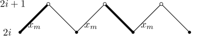
Under the periodic assumption 2, the sets and defined in Definition 2.3 are periodic, so if and only if . Moreover, all the independent edge weights are the ’s for , for the NE-SW edges joining the th and th row (mod ) and the , for , for the NE-SW edges, joining the th and rows. See Figure 2.6. Obviously if and only if .
Lemma 3.8.
For any between 0 and , define , and let
Then the generating Schur function is given by:
Proof 3.9.
We prove the case when is odd here; the case when is even can be proved similarly.
Proposition 3.10.
Assume that the sequence of signatures corresponding the first row is regular, and . Assume that the edge weights for are independent of , while the edge weights satisfy (3.3) or (3.4). Let be a sequence of nonnegative integers such that . Then, the sequence of random measures converges as in probability, in the sense of moments to a deterministic measure in , whose moments are given by
where
| (3.9) |
and the integration goes over a small positively oriented contour around 1.
Proof 3.11.
From Proposition 3.1 it follows that
Let us look at what is happening in the th row, for . Let be the probability measure of perfect matchings along the th row, given that the first row has a configuration . The th row has V-squares. By Lemma 3.8, we have
| (3.10) |
where in the last identity we use the assumption (3.3) or (3.4), and is a fixed finite positive integer relating to the size of the fundamental domain.
3.2. Height function
Let be a contracting square-hexagon lattice.
As for any bipartite planar graph, dimer configurations can be encoded by a height function with values on the faces of the graph. A convenient way to construct a height function (which will help also for the matter of discussing the scaling limit for these graphs), is to see a contracting square-hexagon lattice, as in fact a subgraph of the square lattice, by drawing the vertical edges of the hexagonal rows as diagonal NW-SE (the missing diagonal NE-SW diagonal on these rows correspond to the fusion of two unit squares to make hexagonal faces). The vertices of the contracting square-hexagon graph are thus on the sublattice with coordinates satisfying .
The height function we will consider is then defined on the sublattice where , applying the same rule as for domino tilings [44]: the height increases (resp. decreases) by 1 when going counterclockwise around a white vertex (resp. black vertex), i.e., for half-integer (resp. integer) as long as a dimer is not crossed. For definiteness, we fix the height to be 0 at the square face . When keeping and increasing by one, we jump over a black vertex with two edges, with only one of them being a dimer. Then the height increases by 2. See Figure 3.1. Note that the height function under this definition is a constant multiple of the height function under the classical definition in [28].
The value of the height function can be related directly to the counting measures of the signatures associated to rows of the graph: the height at position is given by the following formula:
If is the signature of the th row (with ordinate ), the numbers are the positions of the , which is (up to a small shift), times the atoms of the counting measure for this signature.
Therefore, if we define , for -half integer, the height along the th row, encoded by the signature , is given by the following formula:
The convergence of the counting measures from Proposition 3.10 implies directly the following theorem about the convergence in probability of the rescaled height:
Theorem 3.12 (Law of large numbers for the height function).
Consider asymptotics such that all the dimensions of a contracting square-hexagon lattice linearly grow with . Assume that
-
•
the sequence of signatures corresponding to the first row is regular, and
in the weak sense; and
- •
Let be the measure on the configurations of the th row, and let , such that , Then converges to in probability as , and the moments of is given by Proposition 3.10.
Define
Then the random height function associated to a random perfect matching , satisfies the following law of large numbers: as goes to infinity, its scaling by a factor
converges uniformly, in probability, to the deterministic function , where are new continuous parameters of the domain.
Remark 3.13.
The continuous variables lie in a region of the plane obtained from by translating each row from the second to the left such that the leftmost vertex of each row are on the same vertical line; then rescaled by , and taking the limit as . When is a square grid, is a rectangle; otherwise is a trapezoid with two right angles on the left.
The convergence also occurs on the other sublattice, when is integer, and half integer, due to the fact that the discrete height function is Lipschitz.
4. Density of the Limit Measure
We work in this section with the same hypotheses as in Theorem 3.12. We obtain an explicit formula to compute the density of the limit of the random counting measure corresponding to the random signatures for dimer configurations on a row of the contracting square-hexagon lattice. This formula for the density of limit measure will be used in the next section to obtain the frozen boundary, i.e., the frontier between frozen regions where the density of the limit measure is 0 or 1, and a temperate region where the density lies strictly between 0 and 1.
Under the assumptions above, it is not hard to check that all the measures , have compact support, and that they is absolutely continuous with respect to the Lebesgue measure on with a density taking values in .
Recall that the Stieltjes transform of a compactly supported measure is defined by
| (4.1) |
for , which has an expansion as a series in in a neighborhood of infinity whose coefficients are the moments of the measure : if the is th moment of , then for large enough:
By Proposition 3.10, we know in principle for any , all the moments of the limiting measure , expressed in terms of the function from Equation (3.9), so we can have an expression of the Stieltjes transform of . However, depends on which is itself expressed in terms of the Stieltjes transform . Indeed, for any measure , the function is is related to the Stieltjes transform of by the following relation:
See also Equation (3.2).
Introducing an additional variable such that , one can then write for :
| (4.2) |
As a consequence, injecting the expression of the moments of the limiting measure into the definition of the Stieltjes transform, one gets an implicit equation to be solved: for any , finding such that
| (4.3) |
allows one to express : let be the composite inverse of
Note that is a uniformly convergent Laurent series in when is in a neighborhood of infinity, and
See Section 4.1 of [8].
The following identity holds when is in a neighborhood of infinity
| (4.4) |
Indeed, by Proposition 3.10, the -th moment of is given by
where the integral is along a small counterclockwise contour winding once around . Then the identity (4.4) follows from the same computation as in the proof of Lemma 4.1 in [8], by performing an integration by parts and a change of variable from to .
The first equation of the system (4.3) with from (4.2) is linear in for given and , which gives with the value of , as a function of , , and :
| (4.5) |
where
| (4.6) |
For a given value , and fixed (and ), we investigate properties of the complex numbers such that . In particular, we have the following:
Lemma 4.1.
Let , for . Let , and . Then the following equation in
| (4.7) |
has roots on the Riemann sphere , where is the number of distinct values of , and all these roots are real and simple.
Proof 4.2.
Let be all the possible distinct values for the , and be their respective multiplicities among the ’s. Define
| (4.8) |
where , with as in Equation (4.6). When writing as a single rational fraction by bringing all the terms onto the same polynomial denominator (of degree ), the polynomial on the numerator has degree at most . So there are at most roots in (and exactly if we add roots at infinity). Notice that the denominator does not depend on and , but just on the ’s.
Moreover, each factor of the form with or is a decreasing function of on any interval where it is defined. As a consequence, on each of the intervals , and , realizes a bijection with . In particular, the equation has a unique solution in every such interval. It is also decreasing on and . Since the limits of when goes to coincide, and
the equation has a unique solution in , which is in fact infinite if and only if the limits of at infinity is zero, that is, when . This gives thus real roots (with possibly one at infinity).
Remark 4.3.
Increasing the value of translates downward the graph of the function . Since is decreasing in any interval of definition, the roots present in the bounded intervals decrease. The one in moves also to the left, and if it started in , when it reaches , it jumps to the right part of and then continues to decrease. In particular, it means that if , the respective roots and are interlaced:
-
•
if ,
-
•
if ,
-
•
if ,
The limiting case when or is equal to is obtained by sending the corresponding root in to .
Rational fractions where zeros of the numerator and denominator interlace have interesting monotonicity properties, already used for example in [40], which are straightforwardly checked by induction using the decomposition of into the sum of simple fractions:
Lemma 4.4.
Let
where and are two sets of real numbers.
-
•
If and satisfy
Then is monotone increasing in each one of the following intervals
-
•
If and satisfy
Then is monotone decreasing in each one of the following intervals
The monotonicity on each interval of definition is still true if has the form:
or
This is helpful to determine the number of solutions of Equation (4.3), as shown in the following lemma:
Lemma 4.5.
Suppose that is a measure with a density with respect to the Lebesgue measure equal to the indicator of a union of intervals , with
Then the system of equations (4.3) has at most one pair of complex (non real) conjugate solutions. Moreover,
-
•
if , for all , then for each fixed , (4.3) has at least distinct real roots;
-
•
if for some in , then for each fixed , (4.3) has at least distinct real roots.
where is the number of distinct s.
Proof 4.6.
The Stieltjes transform can be computed explicitly from the definition:
We use the second expression from (4.5) to substitute in the second equation of (4.3), to get (after exponentiation)
| (4.9) |
Let us suppose that none of the ’s or ’s is equal to . The rational fractions and have the same poles poles (of same order ) and according to Lemma 4.1 have distinct real roots, which by Remark 4.3, interlace. Therefore, the ratio:
is a rational fraction of the form described in the hypotheses of Lemma 4.4. Therefore, on each bounded interval between two consecutive poles, by monotonicity, the graph of the rational fraction will cross the first diagonal exactly once and there are such intervals.
If (no , and exactly) one is equal to , the same argument is applicable. The only difference is that the rational fraction on the right hand side of Equation 4.9 has only zeros, but still poles. Therefore we still get the same number of intersection with the first diagonal, one on each finite interval between two consecutive poles.
If (no and exactly) one is equal to , then this time the rational fraction has finite real poles. Therefore, there is only roots found by this approach between two successive poles.
Remark 4.7.
Note that when rewriting Equation 4.9 as a polynomial equation in , it has degree
Indeed, in the last case, the leading coefficients of the numerator and denominator of the rational fraction are distinct, thus there is no cancellation of the monomials of higher degree when multiplying both sides by the denominator. In both case, it is exactly the number of real roots we found plus 2. Which means that Equation 4.9, and thus Equation 4.3 has at most a pair of complex conjugated roots.
When there are complex conjugated roots, the density of the counting measure is given by their the normalized argument as stated in the Theorem 4.12 below. In order to prove it, we need two additional lemmas, which are minor adaptations of the ones of [8] adapted to our context:
Lemma 4.8.
Let be such that Equation (4.3) has a pair of complex roots. Let be the th smallest real root of (4.3). Let be a small complex neighborhood of . Let be the root of (4.3) approximating , when (which is well defined if is small enough). Then the derivative of with respect to at is non-negative. Moreover, it is equal to 0 if and only if .
Proof 4.9.
Write
then follow the same argument as in the proof of Lemma 4.5 of [8] to show and . Then the lemma follows.
Lemma 4.10.
Proof 4.11.
Here is the main theorem to be proved in this section.
Theorem 4.12.
The density of is given by
where is the unique complex root of the system of equations (4.3) which lies in the upper half plane. If such a complex root does not exist, the density is equal to 0 or 1.
Proof 4.13.
First we assume that is a uniform measure with density one on a sequence of intervals, as described in Lemma 4.5. In this case, the theorem follows from Lemma 4.10, and from the classical fact about Stieltjes transform that if a measure has a continuous density with respect to the Lebesgue measure then one can reconstruct by the following identity (See e.g. [8, Lemma 4.2]):
| (4.10) |
where denote the imaginary part of a complex number.
In the general case of a measure , there exists a sequence of measures converging weakly to , where each is a measure with the form as described in Lemma 4.5. Passing to the limit we obtain the theorem.
5. Frozen Boundary
In this section, we study the frozen boundary, which is the curve separating the “liquid region” and the “frozen region” in the scaling limit of dimer models on a contracting square-hexagon lattice. We prove an explicit formula of the frozen boundary under the assumption that each segment of the boundary row of the square-hexagon lattice grows linearly with respect the dimension of the graph. We then prove that the frozen boundary is a curve of a certain type, more precisely, a cloud curve whose class depends on the size of the fundamental domain and the number of segments of the boundary row. Similar results for dimer configurations on the square grid or the hexagonal lattice with uniform measure or a -deformation of the uniform measure was obtained in [27, 8].
We consider special sequences of contracting square-hexagon lattices with
| (5.1) |
where
In other words, is an -tuple of integers whose entries take values of all the integers in .
We shall consider changing with , and discuss the asymptotics of the frozen boundary as .
Suppose that for each , has corresponding , , for a fixed . Assume also that have the following asymptotic growth:
| (5.2) |
where are new parameters such that .
Definition 5.1.
Let be the set of inside such that the density is not equal to 0 or 1. Then is called the liquid region. Its boundary is called the frozen boundary.
Theorem 5.2.
Proof 5.3.
According to the discussions in Section 4, the frozen boundary is given by the condition that the following equation in the unknown has a double root:
| (5.4) |
where
| (5.5) |
and is defined by Equation (4.8).
We can also rewrite the system of equations (4.3) as follows:
We plug the expression of from the first equation into the second equation, and note that the condition that the resulting equation has a double root is equivalent to the following system of equations
where is defined by (5.3). Then the parametrization of the frozen boundary follows.
The algebraic curve we obtain for the frozen boundary has special properties, that can be read from its dual curve, as described in the definition and the proposition below:
Definition 5.4 ([27]).
A degree real algebraic curve is winding if the following two conditions hold:
-
(1)
it intersects every line in at least points counting multiplicity,
-
(2)
there exists a point called center, such that every line through intersects in points.
The dual curve of a winding curve is called a cloud curve.
Proposition 5.5.
The frozen boundary is a cloud curve of class , where is the number of segments, and is the number of distinct values of in one period. Moreover, the curve is tangent to the following lines in the coordinates:
So the proposition states that the dual curve is winding of degree , and passes through the points and .
The result about the frozen boundary being a cloud curve extends the result of Kenyon and Okounkov [27] for the uniform measure of rhombus tilings of polygonal domains, and Bufetov and Knizel [8] for Aztec rectangles.
Proof 5.6.
We recall that the class of a curve is the degree of its dual curve. So we need to show that the dual curve has degree and is winding.
We apply the classical formula to obtain from a parametrization of the curve defining the frozen boundary, another one for its dual , :
and obtain that the dual curve is given in the following parametric form:
| (5.6) |
from which we can read that its degree is . To show that is winding, we need to look at real intersections with straight lines.
First, from Equation (5.6), one sees that the first coordinate of the dual curve and the parameter are linked by the simple relation .
Using this relation to eliminate from the expression of the second coordinate, we obtain that the points on the dual curve satisfy the following implicit equation:
The points of intersection of the dual curve with a straight line of the form have a parameter satisfying:
| (5.7) |
but since is the composition of two rational fractions and an affine transformation of , with interlacing poles and zeros, with degrees and respectively, the exact same argument as in Lemma 4.8 (but with the role of and exchanged) shows that Equation 5.7 has at least distinct real solutions, yielding points of intersections for the dual curve and the line . Moreover, if doesn’t lie in a compact interval containing all the zeros of , then any non vertical straight line passing through will have intersections with the graph of . See Figure 5.1 for the graph of . This means that for in some closed interval, there are at least real intersections of the dual curve with a line passing through , thus exactly real intersections, since there cannot be a single complex one. Such points are candidates to be the center of the dual curve.
To consider the vertical lines , we rewrite the equations in homogeneous coordinates and get that the line intersects the curve at the point with multiplicity , so again, by the same argument as above, real intersections. The case of the line is similar.
Recall that each point on the dual curve corresponds to a tangent line of . The points belong to . Indeed, they correspond to which is a zero of , and thus of , by (5.3). Similarly, are also points of , since they correspond to which is a pole of , and thus , again by (5.3).
These families of points correspond to the families of tangent lines and . The former are vertical lines passing through , and the latter are lines passing through with slope .
The point corresponds to the tangent line of . By the parametrization of given in Theorem 5.2, the roots of
correspond to points of tangency of with the line .
6. Positions of V-edges in a row and eigenvalues of GUE random matrix
In this section, we prove that near a turning point of the frozen boundary, the present -edges in a random perfect matching of the contracting square-hexagon lattice are distributed like the eigenvalues of a random Hermitian matrix from the Gaussian Unitary Ensemble (GUE).
A matrix of the GUE of size is diagonalizable with real eigenvalues , whose distribution on has a density with respect to the Lebesgue measure on proportional to:
See [34, Theorem 3.3.1]. Here is the main theorem we prove in this section.
Theorem 6.1.
Let be a contracting square-hexagon lattice, such that
-
•
is an -tuple of integers denoting the location of vertices on the first row,
- •
-
•
for every , ,
Let be the signature corresponding to the dimer configuration incident to the th row of white vertices in , and for ,
Let
where is the limit counting measure of signatures on the top of . Let
Then, for any fixed , the distribution of converges weakly to as .
The convergence of the distribution of certain present edges near the boundary to the GUE minor process was proved in [22] in the case of uniform perfect matching on the Aztec diamond, and in [39] for plane partitions. In the case of the uniform perfect matching on a hexagon lattice, the result was proved in [16, 36]. In the case of -distributed perfect matching on a hexagon lattice with , the result was proved in [35].
Proof 6.2 (Proof of Theorem 6.1).
In order to prove Theorem 6.1, we shall apply the following characterization of , which follows directly from the definition. See e.g.[16, 36].
Lemma 6.3.
Let be a random vector with distribution and the diagonal matrix obtained by putting the on the diagonal.
Then is if and only if for any matrix ,
It is in fact enough to check the case when is diagonal, with real coefficients.
Let
By Lemma 2.28, we have for any :
| (6.1) |
Let be the distribution of dimer configurations restricted on the th row of white vertices on , and let
Then
| (6.2) |
the denominator of the last fraction being exactly by Definition 3.3. First, this fraction is converging to 1 as goes to infinity. Indeed, all partitions that contribute to the sum must have parts bounded by a constant times by hypothesis. Since , one has:
uniformly in , which implies that the difference between the fraction and 1 is negligible as goes to .
We then use Lemma 3.8 to re-express the Schur generating function:
| (6.3) |
where is the signature corresponding to the first row.
The same estimate for Schur functions we used before to compare evaluated at and can be used this time for , using the fact that by hypothesis. We have then that
with , so we can, up to a negligible correction, replace in the denominator by in Equation (6.3).
This ratio of Schur functions appears also when using again Lemma 2.28 to rewrite the matrix integral over this time. More precisely, let
where fo . For , let . Then,
| (6.4) |
Expand the sums using the two expansions , and as and tend to 0, to get that:
Then we use Lemma 6.4 below to get the asymptotic behavior of the integral over , to obtain that
where and are respectively the first and second moments of the limiting measure , as goes to infinity. Bringing all the pieces together, and defining
one finally obtain that
Therefore, according to Lemma 6.3, the distribution of the diagonal coefficients of
which are exactly the , converges to .
Lemma 6.4.
Let be fixed. For any , let and
Assume that
-
•
is a regular sequence of signatures,
-
•
as , the counting measures converge weakly to ,
-
•
there exists a fixed positive integer , such that for , =, and
Then as , we have the following asymptotic expansion
| (6.5) |
where is multiplying the th free cumulant of the measure (in particular we have ) and the is the th power sum:
Proof 6.5.
We write as where and is diagonal, with the first coefficients equal to 0 and the others are the s.
From [36, Corollary 6] (see also [17]), there is an asymptotic expansion (at any order) of the left hand side of (6.5)
the first two orders giving the right hand side of (6.5).
We now show that the additional perturbation coming from does not change the first two orders as long as the s are close enough to 1. For this, we rewrite the trace of as:
Then , uniformly in and , and the sum is equal to 1, as is unitary. Therefore, this trace is , and
uniformly in . Thus the correction induced by to the integral is of lower order than the two first terms of the asymptotic expansion above, thus yielding the result.
7. Gaussian Free Field
In this section, we show that under a homeomorphism from the liquid region to the upper half plane, the (non-rescaled) height function of the dimer configurations on a contracting square-hexagon lattice converges to the Gaussian free field (GFF). The relationship between the dimer height function and GFF has been studied extensively in the past few decades. Here is an incomplete list of contributions to this question: the convergence of height functions to GFF in distribution for uniform perfect matchings on a simply-connected domain with Temperley boundary condition was proved in [25, 26]; for random perfect matchings on the isoradial double graph with an analogous Temperley boundary condition was proved in [31]; for uniform perfect matchings on a hexagonal lattice with sawtooth boundary was proved in [3, 42]; for uniform perfect matchings on a square grid with sawtooth boundary (rectangular Aztec diamond) was proved in [8]; for interacting particle systems with non-flat boundary was proved in [12, 13].
7.1. Mapping from the liquid region to the upper half plane
By Theorem 4.12 and Definition 5.1, is in the liquid region if and only if the following system of equations
has non-real roots, where
By explicit computation, one obtains the following:
Lemma 7.1.
Let , where is the upper half plane. Then is the solution of (4.3) if and only if the following equation holds
| (7.1) |
Note that there exists a unique solution of (7.1). Let .
Proposition 7.2.
Let denote the liquid region, and the mapping
sending to the corresponding unique root of (7.1) in . Then, is a homeomorphism with inverse for all , given by
| (7.2) | ||||
| (7.3) |
where
Proof 7.3.
It suffices to show all the following statements:
-
(1)
is nonempty.
-
(2)
is open.
-
(3)
is continuous.
-
(4)
is injective.
-
(5)
has continuous inverse for all .
-
(6)
.
We first prove (1). Explicit computations show that satisfies (7.1). Since is a measure on with compact support, assume that where . The Stieltjes transform satisfies
where and are the first two moments of the measure :
After computations we have
Let be the Lebesgue measure on . Recall that is a probability measure supported in the interval and . Hence we have . Then we infer
Similarly,
As a result, whenever is sufficiently large. Then (1) follows.
7.2. Gaussian Free Field
Let be the space of smooth real-valued functions with compact support in the upper half plane . The Gaussian free field (GFF) on with the zero boundary condition is a collection of Gaussian random variables indexed by functions in , such that the covariance of two Gaussian random variables , is given by
| (7.4) |
where
is the Green’s function of the Laplacian operator on with the Dirichlet boundary condition. The Gaussian free field can also be considered as a random distribution on , such that for any , we have
Here is the Gaussian random variable with respect to , which has mean 0 and variance given by (7.4)) with and replaced by . See [43] for more about the GFF.
Consider a contracting square-hexagon lattice . Let be a signature corresponding to the boundary row.
By (2.10), we defined a probability measure on the set of signatures
By Proposition 2.18, this measure is exactly the probability measure on dimer configurations such that the probability of a perfect matching is proportional to the product of weights of present edges.
Define a function on as follows
This is, up to a deterministic shift, and an affine transformation, the height function defined in Section 3.2, extended to a piecewise constant function.
Let be the push-forward of the measure on with respect to . For , define
Here is the main theorem we shall prove in the section.
Theorem 7.4.
Let be a random function corresponding to the random perfect matching of the contracting square-hexagon lattice, as explained above, with the following hypothesis on the weights :
Then , seen as a random field, converges as goes to to the Gaussian free field in with Dirichlet boundary conditions, in the following sense: for , , define:
and
Then:
7.3. Covariance
To derive this statement, we use the technology developed by Bufetov and Gorin, linking the asymptotic behavior of Schur generating functions to the fluctuations for the related tiling/interlacing signature model [6, 7].
Definition 7.5.
A sequence of symmetric functions is appropriate (or CLT-appropriate) if there exist two collections of real numbers , , such that the following properties are satisfied:
-
•
for any , the function is holomorphic in an open complex neighborhood of , where , and
-
•
for any index and , we have
-
•
For any distinct indices and any , we have
-
•
For any and any indices , such that there are at least three distinct numbers in , we have
-
•
The power series
converge in an open neighborhood of and , respectively.
The definition of CLT-apprioriateness is extended to measures using their Schur gererating functions as follows:
Definition 7.6.
Let as before
satisfying the hypothesis
A sequence of measures is appropriate (or CLT-appropriate) if the sequence of Schur generating functions , defined as in Definition 3.3, is appropriate in the sense of Definition 7.5.
For such a sequence we define functions
Here and are obtained from the definition of CLT-appropriate symmetric functions with as in Definition 7.5.
Lemma 7.7.
Assume that the Schur generating function of a sequence of probability measures on satisfies the conditions
where , are holomorphic functions, and the convergence is uniform in a complex neighborhood of unity. Then is a (CLT-)appropriate sequence of measures with
Let be a positive integer, and be a real number. Let be a probability measure on . Define the random variables
where , and is -distributed.
Theorem 7.8.
Let be an appropriate sequence of measures on signatures with limiting functions and , as defined in Definition 7.6. Then the collection of random variables
converges, as , in the sense of moments, to the Gaussian vector with zero mean and covariance
where
- •
-
•
the - and -contours of integration are counter-clockwise and .
-
•
.
Definition 7.9.
Let . Let be a positive integer and . Let be the space of analytic symmetric functions in the region
where
The space can be considered as a topological space with topology of uniform convergence in the region above. Let
the topological space endowed with the topology of direct limit.
Let be a map with the properties below
-
(1)
is a continuous linear map.
-
(2)
For every ,
-
(3)
For any we have
It follows from (2) and (3) that
Recall that we have a probability measure on dimer configurations of the square-hexagon lattice defined by (2.10), where the square-hexagon lattice has rows and on the bottom row, the configuration has signature . Define a mapping as follows
Let be positive row numbers of the square-hexagon lattice, counting from the top. For , let be the induced probability measure on dimer configurations of the th row. Then the induced probability measure on the state space
by the measure (2.10) can be expressed as follows:
| (7.5) |
where is the probability of conditional on . In particular, we have
where depends on the edge weights. Moreover, we have
and for
For simplicity, we will denote the Schur generating function from Definition 3.3 simply by:
For , let be the Schur generating function for the induced measure on the th row of the .
We use also the following notation for a positive integer .
Lemma 7.10.
Proof 7.11.
The theorem follows from the fact that Schur functions are eigenfunctions for the operators , and explicit computations as in the proof of Proposition 4.3 of [7].
Let be a function with complex variables. Define its symmetrization:
where is the symmetric group of symbols.
Let be a positive integer and let be real numbers. For positive integers and satisfying , we introduce the notation
where is defined by (3.6), and is the Vandermonde determinant on variables .
For a positive integer , let .
Lemma 7.12.
Assume that for each is an analytic function of in an open neighborhood of . Then for any indices the function
| (7.6) |
is analytic in a (possibly smaller) open neighborhood of . If the degree of in is at most (less than ), then the sequence (7.6) has -degree at most (less than ).
Lemma 7.13.
Let be an appropriate sequence of measures on with the corresponding Schur generating function . Let , then
where the degree of in is at most , and the degree of in is less than .
Proof 7.14.
This lemma follows from the same arguments as in the proof of Lemma 5.5 in [7].
For positive integers , satisfying , and , we define
| (7.7) |
For a subset , let be the set of all pairings of the set . Note that if is odd. For a pairing , let be the product over all pairs from this pairing. Finally, for each positive integer let
Proposition 7.15.
Let be an appropriate sequence of measures on , Then for any positive integer , any positive integers , and , for , we have
Proof 7.16.
The proposition follows from the same technique as the proof of Proposition 5.12 in [7], although our definition of Schur generating functions is slightly different.
Proof of Theorem 7.8 The case when for all and was proved in [7, Theorem 2.8]. We will prove it under the assumption that
By Lemma 7.10 and Proposition 7.15, it suffices to show that
| (7.8) |
where by the result in [7], the right hand side of (7.8) is known to be
By definition of an appropriate sequence, see Definitions 7.5, 7.6, we have
From the expression of in (7.7) and the expression of in Lemma 7.13, as well as Lemma 7.12, (7.8) follows.
Lemma 7.17.
Assume that , is a regular sequence of signatures such that
Then
where the convergence is uniform over an open complex neighborhood of .
Proof 7.18.
See Theorem 6.7 of [8].
Proposition 7.19.
Assume that , is a regular sequence of signatures such that
Let such that
| (7.9) |
Then
where the convergence is uniform over an open complex neighborhood of .
Proof 7.20.
Note that
by Lemma 7.17, it suffices to show that
| (7.10) |
Indeed, it suffices to show that the left hand side of (7.10) is independent of . Recall that by Lemma 2.28, we have:
| (7.11) |
We can compute
where
| (7.12) |
Hence it suffices to show that
where is given by
| (7.13) |
Using the same technique as in the proof of Theorem 2.1 in [17], we have
| (7.14) | ||||
| (7.15) | ||||
where the are the double Hurwitz number, see [37]. Under the assumption that is a regular sequence of signatures and (7.9), we have:
Let
then is an analytic function in an open complex neighborhood of . Let
We will compute . Note that only those signatures satisfying contributes to the derivative . In a sufficiently small complex neighborhood of , and when is sufficiently large, by Lemma 7.21 below, we have
Therefore for any there exists an integer , such that for any in an small open complex neighborhood of , and for any satisfying (7.9), for any , we have
| (7.16) |
By the uniform convergence of the derivative we have
As a result,
| (7.17) |
We now state the technical lemma about the generating function of the double Hurwitz numbers:
Lemma 7.21.
Proof 7.22.
See Theorem 3.4 of [17].
Let be a contracting square-hexagon lattice. Let be the row number of a row of counting from the bottom. Then the induced probability measure of dimer configurations on that row is also a measure on Young diagrams given by -tuples. We define the moment function by
| (7.20) |
Theorem 7.23.
The collection of random variables
defined by (7.20), is asymptotically Gaussian with limit covariance
where and ,
Here is the reciprocal of edge weights. Moreover,
8. Examples
In this section, we study a few examples of contracting square-hexagon lattices. By applying the theory developed in previous work and this paper, we explicitly find the limit shapes and the frozen boundaries of perfect matching on these lattices. The examples with parameters are studied in Section 8.1; while the examples with general periodic parameters are studied in Section 8.2.
8.1. Examples with
8.1.1. An Aztec rectangle.
Figure 8.1 shows a domino tiling of a large Aztec rectangle, sampled from the Boltzmann measure with periodic weights given by , , . Here the number of distinct ’s in a period is equal to and the number of distinct parts for the boundary partition is equal to .
This typical tiling, as explained in Section 5, exhibits a spatial phase separation between frozen regions close to the boundary, and a liquid region in the middle. The frozen boundary separating the phases converges in probability to an algebraic curve which, as one can see from Figure 8.1, has tangent points with the bottom boundary. In each interval for of the bottom boundary, the frozen boundary has 2 tangent points, while in each interval for , the frozen boundary has 1 tangent point.
8.1.2. A simple square-hexagon lattice
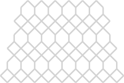
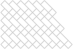
Consider a square-hexagon lattice in which
| (8.1) |
See the left graph of Figure 8.2 for a subgraph of the original square-hexagon lattice, and the right graph Figure 8.2 for a subgraph by translating every row to start from the same vertical line.
Assume that the contracting square-hexagon lattice with satisfying (8.1) has boundary condition specified by
i.e. the boundary partition has three distinct parts of macroscopic size, repeated a macroscopic number of times.
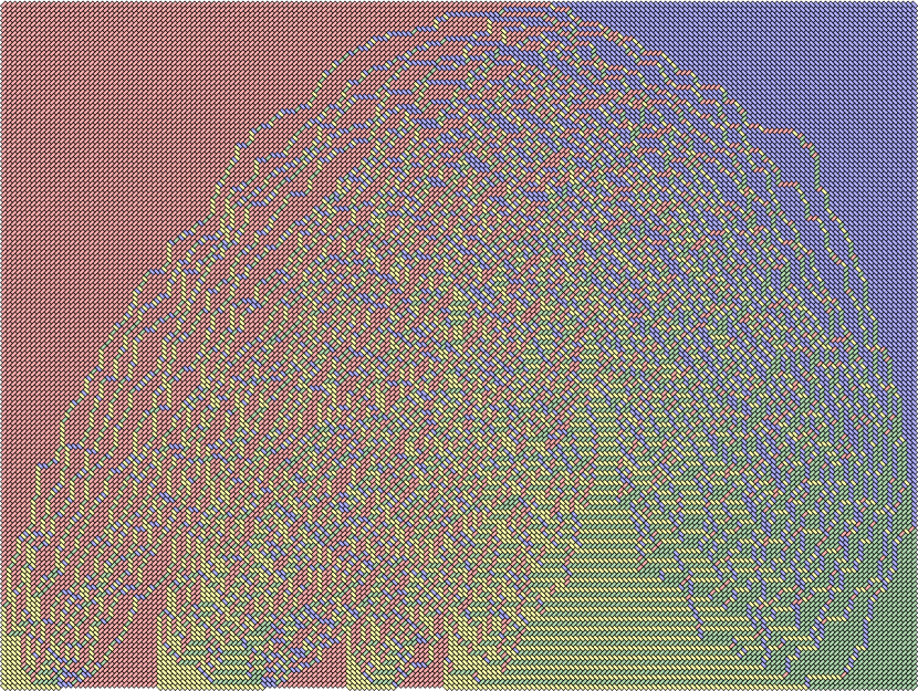
We give two realizations of the dimer model on a large graph on Figures 8.3 and 8.4. Instead of drawing dimers on the graph, we draw only the particles from the bijective correspondence with finite Maya diagrams of Section 2.3.
Figure 8.3 shows the uniform dimer model (i.e. all the edge weights are 1) on a contracting square-hexagon lattice , whereas Figure 8.4 shows a random dimer configuration of the same graph but with periodic weights with a fundamental domain consisting of 8 rows, and edge weights , . We can see that in the periodic case, the frozen boundary has more tangent points with the horizontal line compared to the uniform case.


We may also consider contracting square hexagon lattices with satisfying (8.1) and other boundary conditions. For example, we may consider the counting measures corresponding to the signatures on the bottom boundary converge to a uniform measure on as . Assume that each fundamental domain consists of four rows, , and . In this case we have
Then we solve the equation for and substitute it into (4.3), we have
| (8.2) |
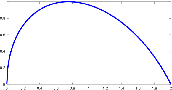
Hence the frozen boundary is given by the condition that the discriminant of (8.2) is 0, which gives
See Figure 8.5 for the frozen boundary in that case, which is not a full closed real algebraic curve inscribed in the domain, contrary to the “stepped case” above.
8.2. An example with
We show on a particular example how computations above can be adapted to take into account situations when the weights do not go to 1. The boundary condition considered is given by a staircase partition where the steps have constant height, not depending on . More precisely, consider a contracting square-hexagon lattice with edge weights assigned as in Proposition 2.18. Assume the configuration on the boundary row is given by the following very specific partition:
| (8.3) |
where is a positive integer. In other words, there are vertices remaining in the boundary row in total; the leftmost vertex and the rightmost vertex are remaining vertices in the boundary row; between each pair of nearest remaining vertices on the boundary row, there are removed vertices. This distribution in the limit as goes to infinity converges to a uniform measure on the whole interval . By [33, Example 1.3.7], we have
when all the ’s are distinct, and extended by continuity when some ’s are equal.
We further assume that the edge weights are assigned periodically with a finite period . That is, for each , and
| (8.4) |
and if ,
| (8.5) |
By Proposition 2.18, the partition function of dimer configurations on the graph can be computed by the following formula
When the edge weights satisfy (8.4) and (8.5), we may compute the free energy as follows, distinguishing the cases where or not in the expression above:
Here we assumed that all the weights ’s in a fundamental domain are distinct. The case when some weights coincide is obtained by continuity.
We can also compute the Schur generating function for the random partition corresponding to the random dimer configuration on each row of the graph, and obtain in this particular case an explicit analogue of Proposition 3.10 giving the moments of the limiting distribution of particles , at macroscopic height .
Let be the distribution of the random partition corresponding to the random dimer configuration on the th row. By Lemma 3.8, we have
for or . When the edge weights are assigned periodically as in (8.4) and (8.5), and letting , , we have
where
Let be a positive integer. Let be the probability measure on the row of the square-hexagon lattice with present -edges, and let be the corresponding random counting measure. Let . Let and satisfying .
Following similar computations as the proof of [6, Theorem 5.1], we have that the leading term for
is given by
First we assume that the edge weights are pairwise distinct. Let
Then
and
Note that
Using residue and following similar computations, we have
where is a simple, closed, positively oriented, contour containing only the poles of the integrand, and no other singularities.
In the case that some of the edge weights may be equal, one has to be separate terms in and introduce instead of the set but at the end, we arrive to the same expression for the moment of .
In [32], it is proved that when the boundary partition differs from (8.3) by at most one component at the beginning, the limit shape is the same as when the boundary partition is given by (8.3).
Define . Adapting again the computations in [6], we can compute the Stieltjes transform of the measure when is in a neighborhood of infinity by
Integration by parts gives
Because has a Laurent series expansion in a neighborhood of given by
has exactly one root in a neighborhood of for , and thus, we can can find a unique composite inverse Laurent series given by
such that when is in a neighborhood of infinity. Then
| (8.6) |
is the unique root of in a neighborhood of .
Since has exactly one zero and one pole in a neighborhood of , we have
and therefore
when is in a neighborhood of infinity. By the complex analyticity of both sides of (8.2), we infer that (8.2) holds whenever is outside the support of .
Lemma 8.1.
Assume the liquid region is nonempty, and assume that for any , has at most one pair of complex conjugate roots. Then for any point lying on the frozen boundary, the equation has double roots.
Proof 8.2.
By Lemma 4.10, the continuous density of the measure with respect to the Lebesgue measure is given by
By (8.2), we have
If the liquid region is nonempty, and for any , has at most one pair of complex conjugate roots, then for each point in the liquid region, there is exactly one of roots from (8.6) converging to a non-real root of ; and all the others converge to real roots of . Then, the lemma follows from the complex analyticity of the density of the limit measure with respect to .
Let us now be more specific with the particular cases when is equal to 1 or 2.
8.2.1.
When , all the vertices on the bottom row are -vertices. Let
where are the distinct values of , with respective multiplicities , and the constant .
Let us call the number of distinct values of ’s for . The equation
| (8.7) |
has at least a real solution for between two consecutive , and between two consecutive (distinct) . This gives at least real roots. As it can be written as a polynomial equation in of degree , we obtain then that Equation (8.7) as at most a pair of complex conjugate roots.
The frozen boundary is given by the condition that the two complex conjugate roots of (8.7) merge to a double root. More precisely, let
Then the frozen boundary has a parametric equation (with parameter ) as follows
Hence we have
| (8.8) |
for on the frozen boundary. The dual curve of the frozen boundary has parametric equation
| (8.9) |
The values of for which the ratio is 0 correspond to horizontal tangency points of the frozen boundary.
For , corresponds to the point of the frozen boundary, and the slope for the corresponding point on the dual curve is 0, because . This gives thus points on the line with horizontal tangent for the frozen boundary.
When is one of the ’s, the corresponding point on the frozen boundary is and the corresponding tangent line is also horizontal. If is the number of distinct ’s in a fundamental domain, then we get horizontal tangency points on the line for the frozen boundary.
By slightly adapting the proof of Proposition 5.5, and checking the definition of cloud curve for this case, one obtains the following
Proposition 8.3.
The frozen boundary given by the parametric equation (8.8) is a cloud curve of rank .
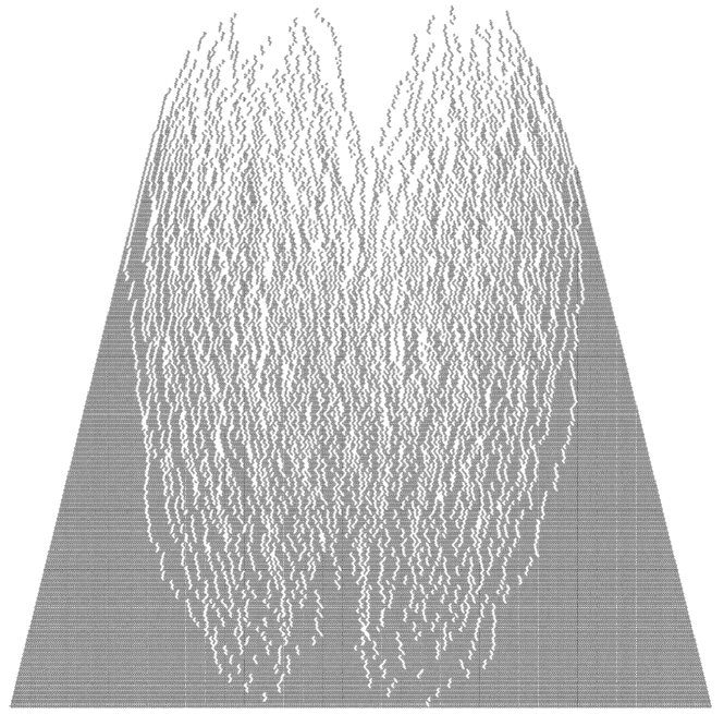
8.2.2.
When , the counting measure on the bottom row converges to the uniform measure on when . Let
As in the case discussed above, Equation (8.7) for has at most one pair of complex conjugate roots, and the parameters for which the two complex conjugate roots merge to a double root correspond to the frozen boundary. More precisely, let
then
for on the frozen boundary. The dual curve of the frozen boundary has parametric equation
If we have distinct values of ’s in the fundamental domain, then for , we get that the points are tangent points of the frozen boundary to the line .

8.3. General Case.
In general, it is possible that the equation has more than one pair of complex conjugate roots. For example, let , , and . In this case, we have
For and , it is not hard to check that the equation has 2 real roots and 4 non-real roots.
References
- [1] A. Borodin, “Schur process and cylindrical partitions”, Duke. Math. J. 140 (2007), p. 391-468.
- [2] ——— , “Schur dynamics of the Schur processes”, Adv. Math. 228 (2011), p. 2268-2291.
- [3] A. Borodin & P. L. Ferrari, “Anisotropic growth of random surfaces in 2 + 1 dimensions”, Commun. Math. Phys. 325 (2014), p. 603-684.
- [4] A. Borodin & P. L. Ferrari, “Random tilings and Markov chains for interlacing particles”, Markov Process. Relat. Fields 24 (2018), no. 3, p. 419-451 (English).
- [5] C. Boutillier, J. Bouttier, G. Chapuy, S. Corteel & S. Ramassamy, “Dimers on rail yard graphs.”, Ann. Inst. Henri Poincaré D, Comb. Phys. Interact. (AIHPD) 4 (2017), no. 4, p. 479-539 (English).
- [6] A. Bufetov & V. Gorin, “Representations of classical Lie groups and quantized free convolution”, Geom.Funct.Anal. 25 (2015), p. 763-814.
- [7] A. Bufetov & V. Gorin, “Fluctuations of particle systems determined by Schur generating functions.”, Adv. Math. 338 (2018), p. 702-781 (English).
- [8] A. Bufetov & A. Knizel, “Asymptotics of random domino tilings of rectangular Aztec diamonds.”, Ann. Inst. Henri Poincaré, Probab. Stat. 54 (2018), no. 3, p. 1250-1290 (English).
- [9] S. Chhita & K. Johansson, “Domino statistics of the two-periodic aztec diamond”, Adv. Math. 294 (2016), p. 37-149.
- [10] H. Cohn, R. Kenyon & J. Propp, “A variational principle for domino tilings”, J. Amer. Math. Soc. 14 (2000), p. 297-346.
- [11] P. Di Francesco & R. Soto-Garrido, “Arctic curves of the octahedron equation”, Journal of Physics A: Mathematical and Theoretical 47 (2014), p. 285204(34pp).
- [12] M. Duits, “The Gaussian free field in an interlacing particle system with two jump rates”, Communications on Pure and Applied Mathematics 66 (2013), p. 600-643.
- [13] ——— , “On global fluctuations for non-colliding processes”, Ann. Probab. 46 (2018), p. 1279-1350.
- [14] E. Duse & A. Metcalfe, “Asymptotic geometry of discrete interlaced patterns. I.”, Int. J. Math. 26 (2015), no. 11, p. 66 (English), Id/No 1550093.
- [15] ——— , “Universalité au bord pour la fluctuation de systèmes discrets de particules entrelacées.”, Ann. Math. Blaise Pascal 25 (2018), no. 1, p. 75-197 (English).
- [16] V. Gorin & G. Panova, “Asymptotics of symmetric polynomials with applications to statistical mechanics and representation theory”, Ann. Probab. 43 (2015), p. 3052-3132.
- [17] I. Goulden, M. Guay-Paquet & J. Novak, “Monotone Hurwitz numbers and the HCIZ integral”, Annales mathematiques Blaise Pascal 21 (2014), p. 71-89.
- [18] A. Guionnet & O. Zeitouni, “Large deviations asymptotics for spherical integrals”, Journal of Functional Analysis 188 (2002), p. 461-515.
- [19] Harish-Chandra, “Differential operators on a semisimple Lie algebra”, Amer. J. Math. 79 (1957), p. 87-120.
- [20] C. Itzykson & J. B. Zuber, “The planar approximation. II.”, J. Math. Phys. 21 (1980), p. 411-421.
- [21] K. Johansson, “The arctic circle boundary and the Airy process”, Ann. Probab. 33 (2005), p. 1-30.
- [22] K. Johansson & E. Nordenstam, “Eigenvalues of gue minors”, Electron. J. Probab. 11 (2006), p. 1342-1371.
- [23] W. Jokusch, J. Propp & P. Shor, “Random domino tilings and the arctic circle theorem”, (1998), \hrefhttps://arxiv.org/abs/math/9801068arXiv:math/9801068.
- [24] P. Kasteleyn, “The statistics of dimers on a lattice, i. the number of dimer arrangements on a quadratic lattice”, Physica 27 (1961), p. 1209-1225.
- [25] R. Kenyon, “Conformal invariance of domino tiling”, Ann. Probab. 28 (2000), p. 759-795.
- [26] ——— , “Dominos and the Gaussian free field”, Ann. Probab. 29 (2001), p. 1128-1137.
- [27] R. Kenyon & A. Okounkov, “Limit shapes and the complex Burgers equation”, Acta Mathematica 199 (2007), p. 263-302.
- [28] R. Kenyon, A. Okounkov & S. Sheffield, “Dimers and amoebae”, Ann. Math. 163 (2006), p. 1019-1056.
- [29] Z. Li, “Fluctuations of dimer heights on contracting square-hexagon lattices”, \hrefhttps://arxiv.org/abs/arXiv:1809.08727arXiv:1809.08727.
- [30] ——— , “Schur function at general points and limit shape of perfect matchings on contracting square hexagon lattices with piecewise boundary conditions”, \hrefhttps://arxiv.org/abs/1807.06175arXiv:1807.06175.
- [31] ——— , “Conformal invariance of dimer heights on isoradial double graphs”, Ann. Inst. Henri Poincáre, Series D 4 (2017), p. 273-307.
- [32] ——— , “Asymptotics of schur functions on almost staircase partitions”, Electron. Commun. Probab. 25 (2020), p. 13pp.
- [33] I. G. Macdonald, Symmetric functions and hall polynomials, Oxford University Press, 1998.
- [34] M. Mehta, Random matrices, Academic Press, 2004.
- [35] S. Mkrtchyan & L. Petrov, “GUE corners limit of -distributed lozenge tilings.”, Electron. J. Probab. 22 (2017), p. 24 (English), Id/No 101.
- [36] J. Novak, “Lozenge tilings and Hurwitz numbers”, J. Stat. Phys. 161 (2015), p. 509-517.
- [37] A. Okounkov, “The Toda equations for Hurwitz numbers”, Mathematical Research letters 7 (2000), p. 447-453.
- [38] A. Okounkov & N. Reshetikhin, “Correlation function of Schur process with application to local geometry of a random 3-dimensional Young diagram”, J. Amer. Math. Soc. 16 (2003), p. 581-603.
- [39] A. Okounkov & N. Reshetikhin, “The birth of a random matrix.”, Mosc. Math. J. 6 (2006), no. 3, p. 553-566 (English).
- [40] A. Okounkov & N. Reshetikhin, “Random skew plane partitions and Pearcey process”, Commun. Math. Phys. 269 (2007), p. 571-609.
- [41] J. K. Percus, “One more technique for the dimer problem”, J. Math. Phys. 10 (1969), p. 1881.
- [42] L. Petrov, “Asymptotics of uniformly random lozenge tilings of polygons. Gaussian free field.”, Ann. Probab. 43 (2015), no. 1, p. 1-43 (English).
- [43] S. Sheffield, “Gaussian free field for mathematicians”, Prob. Theory Relat. Fields 139 (2007), p. 521-541.
- [44] W. P. Thurston, “Conway’s tiling groups”, Amer. Math. Monthly 97 (1990), no. 8, p. 757-773.