Gap states and edge properties of rectangular graphene quantum dot in staggered potential

Abstract

We investigate edge properties of a gapful rectangular graphene quantum dot in a staggered potential. In such a system gap states with discrete and closely spaced energy levels exist that are spatially located on the left or right zigzag edge. We find that, although the bulk states outside the energy gap are nearly unaffected, spin degeneracy of each gap state is lifted by the staggered potential. We have computed the occupation numbers of spin-up and -down gap states at various values of the strength of the staggered potential. The electronic and magnetic properties of the zigzag edges depend sensitively on these numbers. We discuss the possibility of applying this system as a single electron spintronic device.

I Introduction

Graphene exhibits interesting fundamental physicsNeto , such as quantum Hall effectPKim , and BerryAndo and Zak phases. Graphene nanostructures are also important building blocks for device applicationsNeto ; Loss ; Shin ; Sch . In this paper we focus on a nanostructure of a rectangular graphene quantum dot (RGQD) with two armchair edges and two zigzag edgesTang ; Kim . It has several interesting properties. For certain values of the length of the zigzag edges an excitation gap exists that are filled with topological gap statesJeongJNN . These gap states are localized on the zigzag edgesFuj ; Son ; Jeong , and their number grows with the length of the zigzag edges $L_{zig}$Jeong0 . Half of these gap states are localized on the left edge and the other half on the right edge. These gap states are responsible for antiferromagnetism between opposite zigzag edgesTang . In the presence of a weak magnetic field these gap states are no longer localized entirely on the zigzag edges, and can display unexpected patterns in their probability densitiesKim .

In this paper we investigate the effect of a staggered potential of a substratestagpot1 ; stagpot2 ; stagpot3 on the electronic properties of a RGQD with gap states. It has a profound effect on electronic states localized on the zigzag edges. One would expect that, since the opposite zigzag edges experience different electric potentials (see Fig.1), charge imbalance occurs between the left and right zigzag edges, which will in turn affect edge antiferromagnetism. The effect of a staggered potential on the edge states is analogues to the effect of a uniform electric field, but unlike it, a staggered potential does not affect extended states significantly due to its alternating sign, as shown in Fig.1. Its effect has been investigated recently in a periodic zigzag graphene ribbon (PZGR), which has a band crossing at the Fermi energy $E_{F}=0$ when it is half-filled. Depending on the strength of electron-electron interactions, interesting band structures have been found, such as an antiferromagnetic insulating band and antiferromagnetic half metallic band with a non-trivial spin structureSor .

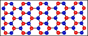
Figure 1: RGQR has two armchair edges and two zigzag edges. The lengths of the armchair and zigzag edges are, respectively, $L_{arm}$ and $L_{zig}$. The staggered potential energy is $\epsilon_{i}=\Delta/2$ on sublattice A (red circles) and $\epsilon_{i}=-\Delta/2$ on sublattice B (blue circles). Note that the opposite zigzag edges experience different potential energies.

In this paper we will explore electronic and magnetic properties of RGQDs with a sizable excitation gap so that gap states are isolated from lower and higher energy quasi-continuum bulk states. These gap states have discrete and closely spaced energy levels, and they are spatially located near the left or right zigzag edge. We find that spin degeneracy of each gap state is broken by the staggered potential. The electronic and magnetic properties of the zigzag edges depend sensitively on the occupation numbers of spin-up and -down gap states. Zigzag edges with different charge imbalance and total spin value are possible for different values of the strength of the staggered potential. For a certain range of the strength of staggered potential $\Delta$ antiferromagnetically coupled zigzag edges exist, but outside this range the electrons in the gap states are all localized only on one zigzag edge. The physics behind the edge magnetism is the competition between lowering of the total staggered potential energy and the energy cost due to the repulsive interactions when electrons move to the edge with the lower staggered potential energy. In contrast to a uniform electric field, a staggered potential does not change significantly the extended states outside the gap.

This paper is organized as follows. In See. II we define our model. Using it we compute gap states in Sec.III. The charge and magnetic configurations of the edges are computed in Sec.IV. Summary and discussion are given in Sec.V.

II Model

Since translational symmetry is broken we write the Hamiltonian in the site representation to compute the groundstate of a RGQD. We adopt a tight-binding model of a RGQD at half-filling with the on-site repulsion $U$ and solve it using the Hartree-Fock (HF) approximation (this approach is widely used and its results are consistent with those of DFTFuj ; Pis ; Yang ). The HF Hamiltonian is

$$H=-t\sum_{ij\sigma}c_{i\sigma}^{{\dagger}}c_{j\sigma}+\sum_{i\sigma}\epsilon_{i}c_{i\sigma}^{{\dagger}}c_{i\sigma}+U\sum_{i\sigma}(n_{i\uparrow}\langle n_{i\downarrow}\rangle+\langle n_{i\uparrow}\rangle n_{i\downarrow}-\langle n_{i\uparrow}\rangle\langle n_{i\downarrow}\rangle),$$ (1)

where $\epsilon_{i}=\pm\Delta/2$, $c_{i\sigma}^{{\dagger}}$ and $n_{i\sigma}$ are the value of the staggered potential at site $i$, electron creation and occupation operators at site $i$ with spin $\sigma$. In the hopping term the summation is over the nearest neighbor sites (the hopping parameter $t\sim 3$ eV). When the length of the zigzag edges is $L_{zig}=(3M+1)a_{0}$ or $3Ma_{0}$ an excitation gap existexptarm ; Brey ; Lee ; Yang ($M$ is an integer and $a_{0}$ is graphene unit cell length). When graphene is epitaxially grown on SiC substrate there is an additional contribution $\Gamma\sim 0.26$ eV to the excitation gap due to the staggered potential stagpot1 . A ribbon with $L_{zig}=(3M+2)a_{0}$ does not have a gap in the absence of electron-electron interactions and will not be considered here. We consider RGQDs with width in the range $\frac{L_{zig}}{L_{arm}}<1$ (when $\frac{L_{zig}}{L_{arm}}\gg 1$ a zigzag ribbon is realized; in this case gap state energies are not well isolated from each other and from the quasi-continuous conduction and valence band states). In general the nature of the gap/edge states state depends on the interplay between several parameters $\Delta$, $U$, $t$, $L_{zig}$, and $L_{arm}$.

III Energy levels of gap states

It is useful to define the number of occupied gap states of spin $\sigma$ located on the left (right) edge $N_{L(R),\sigma}$. In addition, it is helpful to compute the following sums of the occupation numbers for each edge: $N_{L}=N_{L,\uparrow}+N_{L,\downarrow}$ for the left edge and $N_{R}=N_{R,\uparrow}+N_{R,\downarrow}$ for the right edge. The differences of the spin occupation numbers for each edge are defined as $M_{L}=N_{L,\uparrow}-N_{L,\downarrow}$ for the left edge and $M_{R}=N_{R,\uparrow}-N_{R,\downarrow}$ for the right edge.

We compute the energy levels of gap states of a RGQD with $L_{zig}=22.41$Å and $L_{arm}=215.84$Å. For this RGQD there are $12$ gap/end states (counting spins). There are $9$ end sites on each zigzag edge. On each edge, the occupied quasi-continuum states contribute $6$ electrons and the end states contribute $3$ additional electrons, and there are $3+6=9$ electrons in total (note that the system is half-filled and each edge has $9$ sites).

Figure 2(a) displays the energy spectrum of gap states at $\Delta=0$. The numbers of the occupied gap states on the left edge are $(N_{L,\uparrow},N_{L,\downarrow})=(3,0)$ and on the right edge $(N_{R,\uparrow},N_{R,\downarrow})=(0,3)$. The system is antiferromagnetic with $M_{L}=3$ and $M_{R}=-3$ (this antiferromagnetic state is almost degenerate with a ferromagnetic stateTang ). There is no charge imbalance since $N_{L}=3$ and $N_{R}=3$. One spin-down electron transfers discontinuously just after $\Delta=0.026t$. At the transition point two spin-down gap states become degenerate at the Fermi energy. One of them is the highest energy occupied spin-down gap state, that is localized on the left zigzag edge, see Fig.3. The other is the lowest energy unoccupied spin-down gap state that is localized on the right zigzag edge. As we can see Figs.2 and 3 the average energy spacing between the gap states located on the left and right edges becomes smaller as a transition point is approached.

Figure 2(b) displays the schematic energy spectrum of gap states after this transition. Note that the energy spacing between the gap states does not vary uniformly with increasing $\Delta$. The gap occupation numbers are $(N_{L,\uparrow},N_{L,\downarrow})=(3,1)$ and $(N_{R,\uparrow},N_{R,\downarrow})=(0,2)$. The charge imbalance increases: $N_{L}=4$ and $N_{R}=2$. But antiferromagnetism is weakened by this process since the magnitude of total spin on each edge is reduced: $M_{L}=2$ and $M_{R}=-2$.

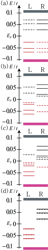
Figure 2: Schematic energy levels of $12$ spin-up and -down gap states are shown at various values of $\Delta/t=0,0.026,0.0267,0.08$ (increasing from (a) to (d)). Solid (dashed) lines represent spin-up (down) gap states. They are all localized on either left (L) or right (R) zigzag edge. On the left edge occupied spin-down gap states increases from $0,1,2$ to $3$ while on the right edge occupied spin-up gap states decreases from $3,2,1$ to $0$. Note that the Fermi energy is $E_{F}=0$. Shaded areas represent quasi-continuum bulk states. The change of the energy position of these states due to the staggered potential is negligible. The energy spacing between the gap states is $\sim 0.01t$. Parameters are $L_{x}=22.41$Å, $L_{y}=215.84$, and $U=0.5t$. Even in the absence of a staggered potential there will be an energy gap and gap states. Outside this gap one has quasi-continuous conduction and valence bands.

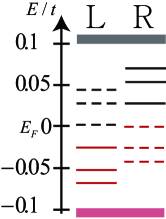
Figure 3: Schematic energy levels of $12$ spin-up and -down gap states are shown at the transition point values $\Delta=0.226t$. Note that two spin-down gap states are degenerate at the Fermi energy. Parameters are same as those given in Fig.2.

There are other two discontinuous changes near $\Delta=0.069t$ and $0.073t$. Figures 2(c) and (d) display the energy spectra of gap states after these transitions. Let us discuss the third electron transfer near $\Delta=0.073t$. Just before the transition the numbers of occupied gap states on the left edge are $(N_{L,\uparrow},N_{L,\downarrow})=(3,2)$ and on the right edge $(N_{R,\uparrow},N_{R,\downarrow})=(0,1)$. Since $M_{L}=1$ and $M_{R}=-1$ the zigzag edges display antiferromagnetism. There is also a charge imbalance: $N_{L}=5$ and $N_{R}=1$. After the transition, one spin-down edge electron is transferred from the right end to the left end: the numbers of occupied gap states on the left edge are $(N_{L,\uparrow},N_{L,\downarrow})=(3,3)$ and on the right edge $(N_{R,\uparrow},N_{R,\downarrow})=(0,0)$. The system is now paramagnetic: $M_{L}=0$ with the maximum charge imbalance $N_{L}=6$ and $N_{R}=0$. We will call this value the critical value of the staggered potential $\Delta_{c}=0.073t$ for $U=0.5t$.

Probability densities of $3$ occupied spin-up gap states localized on the left edge and $3$ occupied spin-down gap states localized on the right edge are also shown in Fig.4.

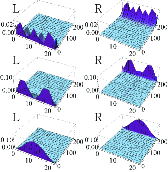
Figure 4: Probability densities of occupied spin-up (left panel) and -down (right panel) gap/edge states are shown (unit of length is Å). They are all localized on either left (L) or right (R) zigzag edge. Other parameters are $L_{x}=22.41$Å, $L_{y}=215.84$, $\Delta=0.026t$ and $U=0.5t$.

IV Electronic and magnetic properties of zigzag edges

We have determined the occupation numbers of the gap states at various values of $\Delta$. Using these numbers we will now calculate electronic and magnetic properties of the zigzag edges. For each spin we compute the average end occupation number per A-site of the right zigzag edge $n_{A,\sigma}$. Note that, in addition to occupied gap states, there are also occupied quasi-continuum bulk states that have to be included in computing this quantity. At a B-site on the opposite end the occupation number $n_{B,\sigma}$ is defined similarly. The average occupation numbers per site of the left and right edges are $n_{L}=n_{A,\uparrow}+n_{A,\downarrow}$ and $n_{R}=n_{B,\uparrow}+n_{B,\downarrow}$. Similarly the average magnetizations per site are $m_{L}=n_{A,\uparrow}-n_{A,\downarrow}$ and $m_{R}=n_{B,\uparrow}-n_{B,\downarrow}$.

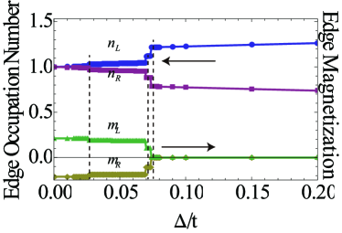
Figure 5: Edge electron occupations per right end site (filled squares) and per left end site (filled circles) of a RGQD are plotted as a function of $\Delta$. Also plotted are the the magnetizations per left end site (diamonds) and per right end site (triangles). A vertical line indicates a value of $\Delta$ where a discontinuous edge reconstruction takes place. On-site potential is $U=0.5t$. Dot length is $L_{arm}=215.84$ Åand width is $L_{zig}=22.41$Å.

Figure 6: Same as in Fig.5 but for $U=0.1t$.

Figure 5 displays $n_{L}$, $n_{R}$, $m_{L}$, and $m_{R}$ for width $22.41$Å, which we used in the last section. At $\Delta=0$, six gap states are occupied: $3$ on the left edge and the other $3$ on the right edge. In addition, on each edge $6$ other electrons are in the occupied quasi-continuum bulk states. So in total $9$ electrons occupy each edge. Three discontinuous transitions are present in the variation of $n_{L}$, $n_{R}$, $m_{L}$, and $m_{R}$. At each discontinuous transition a spin-down edge electron transfers from the right to left edge. After each transition the average occupation per site is approximately $10/9$, $11/9$, and $12/9$. The modification of the occupied quasi-continuum states in response to the staggered potential also contribute to the edge occupation numbers, but only slightly: they contribute to the slowly changing part of $n_{L}$, $n_{R}$, $m_{L}$, and $m_{R}$. Figure 6 displays $n_{L}$, $n_{R}$, $m_{L}$, and $m_{R}$ for a smaller value $U=0.1t$. Note that the critical value $\Delta_{c}=0.014t$ is smaller than that of $U=0.5t$. As in Fig.5 three discontinuous electron transfers are present.

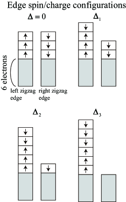
Figure 7: Schematic display of edge spin and charge configurations. Shaded areas represent electrons in the quasi-continuum states and boxes represent gap/edge states. One edge electron moves from the right to left edges at three different values of $\Delta=\Delta_{1},\Delta_{2}$, and $\Delta_{3}$. Shaded areas represent electrons in the quasi-continuum states.

V Summary and discussion

We have computed the closely spaced energy levels of gap states of a RGQD, which are located on the zigzag edges. We find that, although the energy position of the bulk states outside the energy gap is nearly unaffected, spin degeneracy of each gap state is broken by the staggered potential. We have computed the occupation numbers of spin-up and -down gap states at various values of the strength of the staggered potential. Using them we have determined electronic and magnetic properties of zigzag edges. They depend sensitively on the value of the staggered potential. The physical origin of this effect is that an electron on the edge with the high potential energy tend to move to the low potential energy edge, but the electrons on the low potential energy region tend to repel each other. Figure 7 recaptures possible edge electronic and magnetic configurations. At $\Delta=0$ there is no charge imbalance between the edges. Charge imbalance increases suddenly at $\Delta_{1}$, $\Delta_{2}$ and $\Delta_{3}$. The magnitude of the total spin number on the left edge is $M_{L}=3$, $2$, and $1$ at $\Delta=0,\Delta_{1}$, and $\Delta_{2}$, respectively. On the right edge spin values $M_{R}$ are opposite of these, i.e., they are coupled antiferromagnetically with the spins on the left edge. At each transition one spin-down edge electron moves to the left zigzag edge. After the critical value $\Delta_{c}=\Delta_{3}$ antiferromagnetism disappears and $M_{L}=M_{R}=0$. The number of transitions depend on the number of gap states, which is determined by the length of the zigzag edges.

We note several special features of the energy spectrum of the gap states. Unlike a uniform electric field a staggered potential does not affect significantly the quasi-continuum bulk states outside of the gap. Moreover, the energy spacing between the gap states does not vary uniformly with increasing $\Delta$. In a staggered potential the average energy spacing between the gap states located on the left and right edges can become smaller, see Figs.2 and 3. We have also investigated the energy spectrum at several other smaller values of $U/t$. We find at $U/t=0.1$ similar results to those of $U=0.5t$, but the value of the critical strength $\Delta_{c}\sim 0.014t$ is smaller than $\Delta_{c}\sim 0.07t$. The properties of the gap states may be probed using scanning tunneling microscopy measurement of the differential conductanceAndrei .

We conclude by mentioning a possible application of a RGQD in a staggered potential. The authors of Ref.Sor proposed that a long zigzag ribbon in a staggered potential may be used as the electrodes of a tunnel junction of a spin filter. We suggest that a gapful RGQD may be also be used as a single electron spintronic device. For this purpose a small energy spacing between the gap states is desirable. The energy spacing between the gap states becomes smaller for longer zigzag edgesJeong0 and for smaller values of $U$. The energy spacing between the gap states can be made smaller than $0.01t$. A weak electric field will shift the energy levels of the left edge states relative to those of the right edge. When an energy level of the left edge state coincides with that of a right edge state an electron tunneling occurs. By applying an electric field it would thus be possible to modulate the transfer of a spin-down electron from one edge to the other (on the other hand, it would be difficult to modulate the electron transfer by varying the strength of a staggered potential since it is experimentally difficult to change $\Delta$).

References

- (1) A. H. Castro Neto, F. Guinea, N. M. R. Peres, K. S. Novoselov, and A. K. Geim, Rev. Mod. Phys. 81, 109 (2009).
- (2) Y. Zhang, Y.-W. Tan, H. L. Stormer, and P. Kim, Nature 438, 201 (2005).
- (3) T.Ando, J. Phys. Soc. Jpn. 74, 777 (2005).
- (4) B. Trauzettel, D. V. Bulaev, D. Loss and G. Burkard, Nature Physics 3, 192 (2007).
- (5) S. J. Shin, J. J. Lee, H. J. Kang, Jung B. Choi, S.-R. Eric Yang, Y. Takahashi, D. Hasko, Nano Letters , 11 1591 (2011).
- (6) F. Schwierz, Nat. Nanotechnol. 5, 487 (2010).
- (7) C. Tang, W. Yan, Y. Zheng, G. Li, and L. Li, Nanotechnology 19, 435401 (2008).
- (8) S.C. Kim, P.S. Park, and S.-R. Eric Yang, Phys. Rev. B 81, 085432 (2010) .
- (9) Y. H. Jeong and S.-R. Eric Yang, Annals of Physics, to be published.
- (10) M. Fujita, K. Wakabayashi, K. Nakada, K. Kusakabe, J. Phys. Soc. Jpn., 65, 1920 (1996).
- (11) Y. W. Son, M. L. Cohen, and S. G. Louie, Nature 444, 347 (2006).
- (12) Y. H. Jeong, S.C. Kim, and S.-R. Eric Yang, Phys. Rev. B 91, 205441 (2015).
- (13) Y. H. Jeong and S.-R. Eric Yang, Journal of Nanoscience and Nanotechnology 17, 7476 (2017).
- (14) S. Y. Zhou, G.-H. Gweon, A. V. Fedorov, P. N. First, W. A. de Heer, D.-H. Lee, F. Guinea, A. H. Castro Neto, and A. Lanzara, Nature Materials 6, 770 (2007).
- (15) C.R. Dean, A.F. Young, I. Meric, C. Lee, L. Wang, S. Sorgenfrei, K. Watanabe, T. Taniguchi, P. Kim, K.L. Shepard, and J. Hone, Nature Nanotechnology 5, 722 (2010).
- (16) J. Xue, J. Sanchez-Yamagishi, D. Bulmash, P. Jacquod, A. Deshpande, K. Watanabe, T. Taniguchi, P. Jarillo-Herrero, and B. J. LeRoy, Nature Materials 10, 282 (2011).
- (17) D. Soriano and J. Fernández-Rossier, Phys. Rev. B 85, 195433 (2012).
- (18) J. Cai, P. Ruffieux, R. Jaafar, M. Bieri, T. Braun, S. Blankenburg, M. Muoth, A. P. Seitsonen, M. Saleh, X. Feng, K. Müllen, and R. Fasel, Nature 466, 470 (2010); T. Kato and R. Hatakeyama, Nat. Nanotech. 7, 651 (2012).
- (19) L. Brey and H. A. Fertig, Phys. Rev. B 73, 235411 (2006).
- (20) J. W. Lee, S. C. Kim, and S. -R. Eric Yang, Solid State Commun. 152, 1929 (2012).
- (21) L. Yang, C.-H. Park, Y.-W. Son, M. L. Cohen, and S. G. Louie, Phys. Rev. Lett. 99, 186801 (2007).
- (22) L. Pisani, J. A. Chan, B. Montanari, and N. M. Harrison, Phys. Rev. B 75, 064418 (2007).
- (23) E. Y. Andrei, G. Li, and X. Du, Rep. Prog. Phys. 75, 056501 (2012).