Creating anyons from photons using a nonlinear resonator lattice subject to dynamic modulation

Abstract

We study a one-dimensional photonic resonator lattice with Kerr nonlinearity under the dynamic modulation. With an appropriate choice of the modulation frequency and phase, we find that this system can be used to create anyons from photons. By coupling the resonators with external waveguides, the anyon characteristics can be explored by measuring the transport property of the photons in the external waveguides.

Quantum particles satisfy the commutation relation leinaas77

$${\begin{array}[]{*{20}c}a_{j}a_{k}-e^{if(\theta)}a_{k}a_{j}=0,\\ a_{j}a^{\dagger}_{k}-e^{-if(\theta)}a^{\dagger}_{k}a_{j}=\delta_{jk},\\ \end{array}}$$ (1)

where the $a$’s are the annihilation operators. For elementary particles, $f(\theta)$ in Eq. (1) can only take the values of $0$ or $\pi$, corresponding to bosons or fermions respectively. The possibility of creating anyons, described in Eq. (1) by a more complex function of $\theta$, has long fascinated many physicists, both from a fundamental perspective leinaas77 ; goldin81 ; wilczek82 ; wilczek822 ; tsui82 and also due to potential applications in quantum information processing kitaev03 ; sarma05 . Collective excitations that behave as anyons have been constructed from electrons in the fractional quantum Hall systems laughlin83 ; stern08 ; haldane91 , or from atoms in one-dimensional optical lattices keilmann11 ; greschner15 ; strater16 . Moreover, there have been several proposals on using a two-dimensional cavity array to create a fractional quantum Hall effect for photons cho08 ; umucalilar12 ; hafezi13 .

In this letter we propose to construct anyons from photons in a one-dimensional array of cavities. We consider a photonic resonator lattice fang12np ; fang13 ; fang13oe ; lin14 ; yuanprl ; yuanpra with Kerr nonlinearity and moreover is subject to dynamic refractive index modulation fang12 ; fangprb13 ; tzuang14 ; li14 . We show that, with the proper choice of the temporal modulation profile, the Hamiltonian of the system can be mapped into a one-dimensional Hamiltonian for anyons. Moreover, by having the resonator lattice couple to external waveguides (see Figure 1), the resulting open system naturally enable the use of photon transport experiment to measure anyon properties, including a standard beam splitter experiment that can be used to determine particle statistics. Our work opens a new avenue of exploring fundamental physics using photonic structures. The use of a one-dimensional cavity array is potentially simpler to implement as compared to previous works that seek to demonstrate fractional quantum hall effects in two-dimensional cavity arrays. Moreover, the capability for achieving anyon states may point to possibilities for achieving non-trivial many-body photon states that are potentially interesting for quantum information processing. Related to, but distinct from our work, Ref. longhianyon shows that the dynamics of two anyons in a one-dimensional lattice can be simulated with one photon in a two-dimensional waveguide array. But Ref. longhianyon does not construct anyons out of photons.

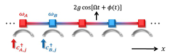
Figure 1: An array of photonic resonators composed of alternating resonators with frequencies $\omega_{A}$ (red) and $\omega_{B}$ (blue). The coupling between nearest-neighbor resonators undergoes dynamic modulation. Each resonator is coupled with an external waveguide.

Our work is inspired by the recent works in the synthesis of anyons in optical lattices keilmann11 ; greschner15 ; strater16 . Consider a Hamiltonian of interacting anyons in one dimension keilmann11

$$H_{A}=-\kappa\sum_{j}\left(a^{\dagger}_{j}a_{j-1}+h.c.\right)+\frac{U}{2}\sum_{j}a^{\dagger}_{j}a^{\dagger}_{j}a_{j}a_{j},$$ (2)

where $\kappa$ is the coupling constant between two nearest-neighbor lattice sites and $U$ is the on-site interaction potential. $a^{\dagger}_{j}$($a_{j}$) is the creation (annihilation) operator for the anyon at the $j$-th lattice site, which satisfies the commutation relations of Eq. (1) with $f(\theta)=\theta\mathrm{sgn}(j-k)$ where $\theta\in[0,2\pi]$. The anyonic Hamiltonian in Eq. (2) can be mapped to the bosonic Hamiltonian

$$H_{B}=-\kappa\sum_{j}\left(b^{\dagger}_{j}b_{j-1}e^{i\theta b^{\dagger}_{j}b_{j}}+h.c.\right)+\frac{U}{2}\sum_{j}b^{\dagger}_{j}b^{\dagger}_{j}b_{j}b_{j},$$ (3)

with the bosonic creation (annihilation) operator $b^{\dagger}$($b$), under the generalized Jordan-Wigner transformation batchelor06 ; kundu99

$$a_{j}=b_{j}\exp\left(i\theta\sum_{m=j+1}b^{\dagger}_{m}b_{m}\right).$$ (4)

Therefore, to create anyon one needs a bosonic system with a particle-number-dependent hopping phase that breaks mirror and time-reversal symmetry.

Ref. strater16 showed that the Hamiltonin in Eq. (3) can be achieved by considering a time-dependent Hamiltonian

$$H(t)=-g\sum_{j}\left(b^{\dagger}_{j}b_{j-1}+h.c.\right)+\frac{V}{2}\sum_{j}b^{\dagger}_{j}b^{\dagger}_{j}b_{j}b_{j}+\left[\Delta\omega+F(t)\right]\sum_{j}jb^{\dagger}_{j}b_{j},$$ (5)

in the weak perturbation limit $g,|U|\ll\Delta\omega$. Here $g$ is the coupling constant, $V=U+2\Delta\omega$ is the interaction potential, $\Delta\omega$ is the potential tilt in the lattice, and $F(t)=-d\phi(t)/dt$, where $\phi(t)=p\cos(\Delta\omega t)+q\cos(2\Delta\omega t)$. In the limit where only one or two-particle processes are significant, and under the high frequency approximation, the Hamiltonian of Eq. (5) maps to that of Eq. (3), provided that the parameters $p$ and $q$ are appropriately chosen. Briefly, in Eq. (5), the time-periodic force $F(t)$ is resonant with the tilted potential difference between nearest-neighbor lattice sites. And the presence of on-site interaction results in the particle-number-dependent phase in the coupling matrix elements after a gauge transformation is carried out strater16 .

Building upon the previous works as outlined above, the main contributions of the present paper are: (1) we show that the one-dimensional Hamiltonian of Eq. (5), including its specific choice of parameters required for anyon synthesis, can be implemented in a photonic structure composed of resonators undergoing modulation. (2) Implementing Eq. (5) in a photonic resonator lattice also points to new possibilities for probing the physics of anyons. In particular, coupling the resonator to an external waveguide (Figure 1) enables one to directly conduct anyon interference experiments, and to probe anyon density distributions of both ground and excited states through a photon transport measurement.

We consider a photonic resonator lattice composed of two kinds of resonators ($A$ and $B$) with frequencies $\omega_{A}$ and $\omega_{B}$ as shown in Figure 1 fang12np . The coupling between nearest-neighbor resonators undergoing dynamic modulation. Such a dynamic modulation of coupling can be implemented using refractive index modulation as discussed in Ref. fang12np . Each resonator moreover has Kerr nonlinearity. Such a system is described by the Hamiltonian $H_{r}$:

$$H_{r}=\sum_{m}\omega_{A}b^{\dagger}_{A,m}b_{A,m}+\sum_{n}\omega_{B}b^{\dagger}_{B,n}b_{B,n}-\sum_{\langle mn\rangle}2g\cos[\Omega t+\phi(t)]\left(b^{\dagger}_{A,m}b_{B,n}+h.c.\right)$$

$$+\frac{V}{2}\sum_{m}b^{\dagger}_{A,m}b^{\dagger}_{A,m}b_{A,m}b_{A,m}+\frac{V}{2}\sum_{n}b^{\dagger}_{B,n}b^{\dagger}_{B,n}b_{B,n}b_{B,n},$$ (6)

$b^{\dagger}$($b$) is the creation (annihilation) operator for the photon in the sublattice $A$ and $B$. The third term in Eq. (6) describes the modulation. $g$ and $\Omega$, and $\phi(t)$ are the strength, the frequency and the phase of the modulation respectively. We assume a near-resonant modulation with $\Omega\approx\omega_{A}-\omega_{B}$. The last two terms describe the effect of Kerr nonlinearity with $V$ characterizes the strength of the nonlinearity.

With the rotating-wave approximation and defining $\tilde{b}_{m}=b_{A,m}e^{i\omega_{A}t}$ ($\tilde{b}_{n}=b_{B,n}e^{i\omega_{B}t}$), we can transform Hamiltonian (6) to

$$\tilde{H}_{r}=-g\sum_{j}\left(\tilde{b}^{\dagger}_{j}\tilde{b}_{j-1}e^{i\Delta\omega t-\phi(t)}+h.c.\right)+\frac{V}{2}\sum_{j}\tilde{b}^{\dagger}_{j}\tilde{b}^{\dagger}_{j}\tilde{b}_{j}\tilde{b}_{j},$$ (7)

where $\Delta\omega=(\omega_{A}-\omega_{B})-\Omega$ is the detuning.

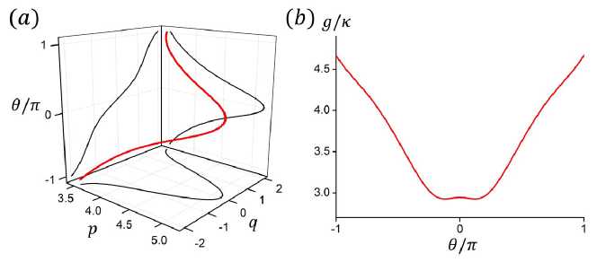
Figure 2: (a) The trajectory that parameters $p,q$ in the modulation phase ($\phi(t)=p\cos(\Delta\omega t)+q\cos(2\Delta\omega t)$) obey, for the Hamiltonian (6) to map into Hamiltonian (3) in the two-photon limit, with $\theta$ in Eq. (3) varying from $-\pi$ to $\pi$. (b) The adjustment of the modulation strength $g$ versus $\theta$ to achieve a constant $\kappa$ in Eq. (3).

Hamiltonians in Eqs. (5) and (7) are equivalent after a gauge transformation $\hat{U}(t)=\exp\left\{i\left[\Delta\omega t-\phi(t)\right]\sum_{j}j\tilde{b}^{\dagger}_{j}\tilde{b}_{j}\right\}$. Since, with proper choice of parameters, Ref. strater16 showed that Eq. (5) can be mapped to the anyon Hamiltonian of Eq. (3), we have shown that a nonlinear photonic resonator lattice undergoing dynamic modulation in fact can be used to construct anyons from photons. In Eq. (6), the near-resonant modulation results in the coupling between resonators at different sites in the lattice. The small detuning between the modulation frequency and the frequency difference $\omega_{A}-\omega_{B}$ results in a tilt potential along the lattice yuanOptica ; longhi05 . The additional time-dependent modulation phase $\phi(t)$ provides the time periodic force. For the rest of the paper, we chose $\Delta\omega=V/2$. In the two-photon limit, $\tilde{H}_{r}$ in Eq. (7) then provides an anyon Hamiltonian of Eq. (3) that is non-interacting with $U=0$. Here choices of parameters $p,q$ as well as $g$ follow the trajectories in Figure 2. $\theta$ can be tuned from $0$ to $2\pi$ following the trajectory of $p,q$ in Figure 2(a). For each $\theta$, $g$ is chosen following Figure 2(b) such that $\kappa$ in Eq. (3) remains constant.

The photonic resonator lattice provides a unique platform for probing the physics of anyons. By coupling the nonlinear resonator as discussed above with the external waveguide (Figure 1), it becomes possible to demonstrate anyon physics through photon transport measurement. The cavity-waveguide system is described by the Hamiltonian:

$$H=\sum_{m}\int_{k}dk\omega_{k}c^{\dagger}_{k,A,m}c_{k,A,m}+\sum_{n}\int_{k}dk\omega_{k}c^{\dagger}_{k,B,n}c_{k,B,n}$$

$$+\sqrt{\frac{\gamma}{2\pi}}\sum_{m}\int_{k}dk\left(c^{\dagger}_{k,A,m}+c_{k,A,m}\right)\left(b^{\dagger}_{A,m}+b_{A,m}\right)+\sqrt{\frac{\gamma}{2\pi}}\sum_{n}\int_{k}dk\left(c^{\dagger}_{k,B,n}+c_{k,B,n}\right)\left(b^{\dagger}_{B,n}+b_{B,n}\right)$$

$$+H_{r}\left[b_{A,m},b_{B,n}\right],$$ (8)

where $c^{\dagger}_{k}$($c_{k}$) is the creation (annihilation) operator for the photon in the waveguide coupled with the $m(n)$-th resonator of type $A(B)$. $\gamma$ is the waveguide-cavity coupling strength. The Hamiltonian of the resonator lattice $H_{r}\left[b_{A,m},b_{B,n}\right]$ is given in Eq. (6). By applying the rotating-wave approximation with $\tilde{c}_{k,m}=c_{k,A,m}e^{i\omega_{A}t}$ ($\tilde{c}_{k,n}=c_{c,B,n}e^{i\omega_{B}t}$), we rewrite Eq. (8) to

$$\tilde{H}=\sum_{j}\int_{k}dk\left(\omega_{k}-\omega_{A(B)}\right)\tilde{c}^{\dagger}_{k,j}\tilde{c}_{k,j}+\sqrt{\frac{\gamma}{2\pi}}\sum_{j}\int_{k}dk\left(\tilde{c}^{\dagger}_{k,j}\tilde{b}_{j}+\tilde{b}^{\dagger}_{j}\tilde{c}_{k,j}\right)+\tilde{H}_{r}\left[\tilde{b}_{j}\right],$$ (9)

where $\tilde{H}_{r}\left[\tilde{b}_{j}\right]$ is given in Eq. (7) fan10 ; yuanOL15 .

The photon transport properties of Eq. (9) can be described by the input-output formalism, which is a set of operator equations in the Heisenberg picture: fan10

$$\frac{d\tilde{b}_{j}(t)}{dt}=i\left[\tilde{H}_{r},\tilde{b}_{j}(t)\right]-\frac{\gamma}{2}\tilde{b}_{j}(t)+i\sqrt{\gamma}c_{in,j}(t),$$ (10)

$$c_{out,j}(t)=c_{in,j}(t)-i\sqrt{\gamma}\tilde{b}_{j}(t).$$ (11)

Here $c_{in,j}$ and $c_{out,j}$ are the input and output operators for waveguide photons gardiner85m .

To probe anyon property one needs at least two particles. We therefore consider a normalized input state

$${\begin{array}[]{*{20}c}|\Phi\rangle=\iint dt_{1}dt_{2}\chi(t_{1}-t_{2})\eta\left(\frac{t_{1}+t_{2}}{2}\right)c^{\dagger}_{in,\alpha}(t_{2})c^{\dagger}_{in,\beta}(t_{1})|0\rangle,&&&(j\leq m)\\ \end{array}}$$ (12)

where the normalization condition $\langle\Phi|\Phi\rangle=1$ requires that $\iint dtdt^{\prime}\chi^{2}(t^{\prime})|\eta(t)|^{2}=1$. In what follows, we assume that $\chi(t)$ has a very short temporal width to describe a scenario where we simultaneously inject two photons into $\alpha$-th and $\beta$-th cavities through the waveguides. In the presence of such input state, we can compute the resulting two-photon probability amplitude inside the resonator lattice

$${\begin{array}[]{*{20}c}v_{jm}(t)\equiv\langle 0|\tilde{b}_{m}(t)\tilde{b}_{j}(t)|\Phi\rangle,&&&(j\leq m)\\ \end{array}},$$ (13)

which from the input-output formalism satisfies (details in the Appendix):

$$\frac{dv_{jm}(t)}{dt}=i\langle 0|\left[\tilde{H}_{r},\tilde{b}_{m}(t)\tilde{b}_{j}(t)\right]|\Phi\rangle-\gamma v_{jm}(t)-\gamma\eta(t)\delta_{j\alpha}\delta_{m\beta}.$$ (14)

The two-photon probability amplitude in (13) can be measured by coupling the resonator lattice to additional output waveguides, and measuring the two-photon correlation function for the photons in the output waveguides.

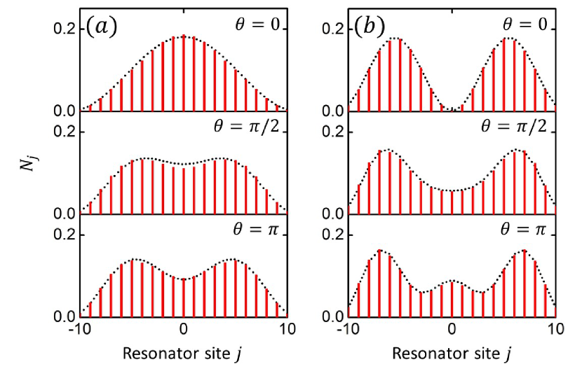
Figure 3: (a) the ground-state and (b) the 2nd excited-state particle density distributions $N_{j}$ for $\theta=0,\pi/2,\pi$ respectively with an input photon pair. $N_{j}$ is normalized to $\sum_{j}N_{j}=2$. The density distributions are compared with the results obtained by a direct diagonalization of the anyon Hamiltonian of Eq. (2) (dotted curves).

Using Eq. (14), we then propose a set of photon transport experiments to probe the anyon statistics. When two anyons are confined in a potential well, the probability distribution of the eigenstates has characteristics that depends on the phase angle $\theta$. Previous proposal on anyon in optical lattice has focused on ground state characteristics keilmann11 ; greschner15 ; strater16 . In our case, on the other hand, one can choose the frequency detuning $\epsilon$ of the input source to selectively excite either the ground state or the excited states. As an illustration, we choose $\eta(t)=e^{-i\epsilon t}\left[u(t)+u(T-t)-1\right]/\sqrt{T}$ in Eq. (12) where $u(t)$ is the Heaviside step function and simulate Eq. (14) to obtain steady-state density distribution $N_{j}=\langle\Phi|\tilde{b}^{\dagger}_{j}(t)\tilde{b}_{j}(t)|\Phi\rangle=\sum_{m<j}|v_{mj}(t)|^{2}+\sum_{m>j}|v_{jm}(t)|^{2}+2|v_{jj}(t)|^{2}$. In the simulation, we consider a lattice involving 21 resonators ($j=-10,\ldots,10$), and choose parameters $\gamma=0.002\kappa$, $\Delta\omega=100\pi\kappa$, and $T=5/\gamma$. To probe the ground state distribution, we use the input state in (12) with $\alpha=-4$, $\beta=4$ and $\epsilon=-3.96\kappa,-3.91\kappa,-3.90\kappa$ for $\theta=0,\pi/2,\pi$ respectively (see Figure 3(a)). When $\theta=0$, the particle density distribution has the distribution with one peak in the $0$-th resonator, which is consistent with the characteristic of bosonic particles. On the other hand, when $\theta=\pi$, the particle density distribution has two peaks near the $\pm 5$-th resonators, corresponding to the characteristic of two non-interacting fermionic particles. The case of $\theta=\pi/2$ has a distribution that is between the boson and the fermion cases. The simulation results by computing Eq. (14) match with the results obtained by a direct diagonalization of the anyon Hamiltonian of Eq. (2). We note that the simulation of Eq. (14) describes an open quantum system, whereas Eq. (2) describes a closed quantum system. Therefore, we show that with proper choice of system parameters, one can use the open system to probe the properties of a closed system. Similar agreement between the photonic resonator lattice system and the anyon Hamiltonian can be seen in excited-state properties as well, as can be seen in Figure 3(b), where as an example we selectively excite the 2nd excited state by setting $\alpha=-6$, $\beta=6$ and $\epsilon=-3.84\kappa,-3.78\kappa,-3.74\kappa$ for $\theta=0,\pi/2,\pi$ respectively in Eq. (12). We note that in addition to the frequency detuning a different choice of the input state distribution is required in order to efficiently excite either the ground state or a particular excited state.

Arguably the most direct experiment for observing particle statistics is the two-particle scattering experiments at a 50/50 beam splitter hong87n ; liu98n ; loudon98 . Consider two quantum particles arriving simultaneously at the beam splitter from both sides (Figure 4(a)). Upon scattering at the beam splitter, for bosons the two particles appear at the same side of the beam splitter. For fermions, the two particles appear at the opposite sides. For anyons, depending on the phase angle $\theta$, the outcome smoothly interpolates between the cases of bosons and fermions. While conceptually simple, there has not been a proposal for conducting such a two-particle scattering experiment for synthetic anyons, due in part to the difficulty of obtaining individual anyons in either electronic or atomic systems.

We show that the cavity-waveguide system can be used to perform the two-anyon interference experiment. For the input, we consider two photons injected into the $1$-st and $-1$-st waveguides, respectively. These two waveguide channels correspond to the two input ports in the standard interferometer experiment. We consider the output photon at $0$-th waveguide which emits from the $0$-th photonic resonator. The $0$-th waveguide channel represents one of the output ports. We define two-photon correlation function $G_{j}^{(2)}(t,\tau)=\langle\Phi|c_{out,j}^{\dagger}(t)c_{out,j}^{\dagger}(t+\tau)c_{out,j}(t+\tau)c_{out,j}(t)|\Phi\rangle$. The total probability that two output photons at $0$-th waveguide coincide in time is then:

$$P_{j=0}\equiv\int dtG_{j=0}^{(2)}(t,\tau=0)=\gamma^{2}\int dt\langle\Phi|\tilde{b}_{0}^{\dagger}(t)\tilde{b}_{0}^{\dagger}(t)\tilde{b}_{0}(t)\tilde{b}_{0}(t)|\Phi\rangle=\gamma^{2}\int dt|v_{00}(t)|^{2}.$$ (15)

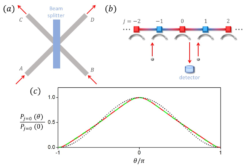
Figure 4: (a) A beam splitter with input arms A and B as well as output arms C and D. (b) The cavity-waveguide system, two photons are incident into the $1$-st and $-1$-st waveguides. The detection is performed at the $0$-th waveguide. (c) Simulated $P_{j=0}$ versus $\theta$ from $0$ to $2\pi$ using $\tilde{H}_{r}$ in Eq. (14) (red solid curve), and the time-independent Hamiltonian $H_{B}$ in Eq. (3) with $U=0$ (green dashed curve). Black dotted curve corresponds to $\cos^{2}(\theta/2)$ as obtained from a simple approximation.

We simulate the “beam splitter” experiment by solving Eq. (14). For the resonator lattice, we used the same parameters as in Figure 3 except for $\gamma=0.25\kappa$. For the input state, we use $\eta(t)=\left(2/\pi T^{2}\right)^{1/4}\exp\left(-t^{2}/T^{2}\right)$ where $T=0.0425\kappa^{-1}$. We plot the simulated $P_{j=0}$ in Figure 4(c). We compare such results to the case where replace $\tilde{H}_{r}$ in Eq. (14), with the time-independent Hamiltonian $H_{B}$ in Eq. (3) with $U=0$. The two simulations show excellent agreement. Since $H_{B}$ is rigorously equivalent to the anyon Hamitonian of Eq. (2). Our simulation results prove that the cavity-waveguide Hamitonian can indeed generate anyonic behavior in spite of all the approximates used to map Eq. (7) to Eq. (3).

The results in Figure 4(c) can be qualitatively accounted for with a simple two-particle interference model. Our choice of the input state results in an excitation of the $1$-st and $-1$-st resonators in the lattice:

$${\begin{array}[]{*{20}l}|\Psi\rangle&=\frac{1}{2}\left(\tilde{b}^{\dagger}_{-1}\tilde{b}^{\dagger}_{1}|0\rangle+\tilde{b}^{\dagger}_{1}\tilde{b}^{\dagger}_{-1}|0\rangle\right)\\ &=\frac{1}{2}\left(e^{i\theta}a^{\dagger}_{-1}a^{\dagger}_{1}|0\rangle+a^{\dagger}_{1}a^{\dagger}_{-1}|0\rangle\right)\\ \end{array}}$$ (16)

where Eq. (4) is used to transform the bosonic to the anyonic operators. Upon time evolution, the state acquires a component in the $0$-th resonator of approximately the form: $\frac{1}{2}\left(e^{i\theta}+1\right)\left(a^{\dagger}_{0}\right)^{2}|0\rangle$. Thus $G_{j=0}^{(2)}(t,\tau=0)\approx\cos^{2}(\theta/2)$ at the $0$-th waveguide as shown in Figure 4(c). This simple model, where the phase factor $\theta$ appears explicitly due to anyon exchange, provides a qualitative explanation of the numerical results show in Figure 4(c). In particular, both the analytic model and the numerical results indicate a peak of $P_{j=0}$ at $\theta=0$, corresponding to the boson case, and $P_{j=0}=0$ at $\theta=\pi$, corresponding to the fermion case. Our results here indicate that one can indeed perform a two-anyon interference experiment using photons in the cavity-waveguide system.

To implement the concepts presented above experimentally, we note that the experimental feasibility of Hamiltonian in Eq. (6), without the nonlinear term, has been discussed in details in Ref. fang12np . For our purpose here, the frequency difference between two resonators of different types can be chosen as $\omega_{A}-\omega_{B}\sim 1$ GHz. The dynamic modulation is applied with the modulation detuning $\Delta\omega\sim 100$ MHz and the modulation strength $g\sim 10$ MHz. Such a modulation strength and speed is consistent with what is achievable in experiments based on silicon electro-optic modulators tzuang14 ; tzuangnewOL ; reednewNP . We also estimate the relevant experimental parameters for the nonlinear term. In Ref. strater16 , in order to obtain Eq. (3) from Eq. (5), one needs to assume $|V-2\Delta\omega|\ll\Delta\omega$, therefore the nonlinearity parameter $V\sim 2\Delta\omega$, which means that adding an extra photon in the resonator will shift the resonant frequency of the resonator by approximately 100 MHz. Such a strength of nonlinearity can be achieved by coupling a two-level quantum system with a resonator and reaching the strong coupling regime chang14 ; imamoglu97 ; carusotto09 . The nonlinear parameter in the range $10$ MHz $\sim$ $10$ GHz have been demonstrated in the recent atom-cavity experiments birnbaum05 ; fushman08 ; kubanek08 ; koch11 ; volz12 , which is sufficient for our experimental proposal.

In summary, we propose a mechanism to achieve one-dimensional anyon from photons by using a nonlinear photonic resonator lattice under dynamic modulation. With this mechanism, both the ground state and the excited states of the anyon system can be selectively probed. Our system also enables the use of a two-photon interference experiment to directly probe the statistics of anyons. This platform can be useful for demonstrating a wide variety of other anyon physics effects hao08 ; hao12 ; wright14 ; tang15 , such as quantum works of two interacting anyons wang14 , and Bloch oscillation of anyons longhibloch12 , that are potentially important for quantum information processing castagnoli93 ; mochon04 ; nayak08 ; alicea11 ; duric17 . On the other hand, we also note that the present proposal represents a simulation of anyon physics in one-dimensional systems. Some of the topological properties associated with anyons in higher dimensions may not be preserved in such simulations bardyn12 .

* Those two authors contributed equally to this work.

Appendix — Equations for two-photon amplitudes inside the cavity as derived from the input-output formalism

The photon transport properties of Eq. (9) can be described by the input-output formalism, which is a set of operator equations in the Heisenberg picture: fan10 ; gardiner85m

$$\frac{d\tilde{b}_{j}(t)}{dt}=i\left[\tilde{H}_{r},\tilde{b}_{j}(t)\right]-\frac{\gamma}{2}\tilde{b}_{j}(t)+i\sqrt{\gamma}c_{in,j}(t),$$ (A-1)

$$c_{out,j}(t)=c_{in,j}(t)-i\sqrt{\gamma}\tilde{b}_{j}(t),$$ (A-2)

where

$$c_{in,j}(t)\equiv\lim_{t_{0}\rightarrow-\infty}\int dk\tilde{c}_{k,j}(t_{0})e^{-ik(t-t_{0})}/\sqrt{2\pi}$$ (A-3)

$$c_{out,j}(t)\equiv\lim_{t_{1}\rightarrow\infty}\int dk\tilde{c}_{k,j}(t_{1})e^{-ik(t-t_{1})}/\sqrt{2\pi}.$$ (A-4)

We can re-write Eq. (A-1) as

$$\tilde{b}_{j}(t)=\tilde{b}_{j}(-\infty)+i\int_{-\infty}^{t}dt^{\prime}\left\{\left[\tilde{H}_{r},\tilde{b}_{j}(t^{\prime})\right]+i\frac{\gamma}{2}\tilde{b}_{j}(t^{\prime})\right\}+i\sqrt{\gamma}\int_{-\infty}^{t}dt^{\prime}c_{in,j}(t^{\prime}).$$ (A-5)

Using Eqs. (A-1) and (A-5), we obtain

$$\frac{d\tilde{b}_{m}(t)\tilde{b}_{j}(t)}{dt}=i\left[\tilde{H}_{r},\tilde{b}_{m}(t)\tilde{b}_{j}(t)\right]-\gamma\tilde{b}_{m}(t)\tilde{b}_{j}(t)$$

$$+i\sqrt{\gamma}\tilde{b}_{m}(-\infty)c_{in,j}(t)-\sqrt{\gamma}\int_{-\infty}^{t}dt^{\prime}\left\{\left[\tilde{H}_{r},\tilde{b}_{m}(t^{\prime})\right]+i\frac{\gamma}{2}\tilde{b}_{m}(t^{\prime})\right\}c_{in,j}(t)-\gamma\int_{-\infty}^{t}dt^{\prime}c_{in,m}(t^{\prime})c_{in,j}(t)$$

$$+i\sqrt{\gamma}c_{in,m}(t)\tilde{b}_{j}(-\infty)-\sqrt{\gamma}\int_{-\infty}^{t}dt^{\prime}c_{in,m}(t)\left\{\left[\tilde{H}_{r},\tilde{b}_{j}(t^{\prime})\right]+i\frac{\gamma}{2}\tilde{b}_{j}(t^{\prime})\right\}-\gamma\int_{-\infty}^{t}dt^{\prime}c_{in,m}(t)c_{in,j}(t^{\prime}).$$ (A-6)

To probe anyon property one needs at least two particles. We therefore consider a normalized input state

$${\begin{array}[]{*{20}c}|\Phi\rangle=\iint dt_{1}dt_{2}\chi(t_{1}-t_{2})\eta\left(\frac{t_{1}+t_{2}}{2}\right)c^{\dagger}_{in,\alpha}(t_{2})c^{\dagger}_{in,\beta}(t_{1})|0\rangle,&&&(j\leq m)\\ \end{array}}$$ (A-7)

where the normalization condition $\langle\Phi|\Phi\rangle=1$ requires that $\iint dtdt^{\prime}\chi^{2}(t^{\prime})|\eta(t)|^{2}=1$. In what follows, we assume that $\chi(t)$ has a very short temporal width to describe a scenario where we simultaneously inject two photons into $\alpha$-th and $\beta$-th cavities through the waveguides. Such an input state corresponds to a strongly-correlated photon pair. Such an input state can be prepared by the four-wave-mixing process ramelow09s ; li09s ; silverstone14s ; kim15s .

In the presence of such input state, we can compute the resulting two-photon probability amplitude inside the resonator lattice

$${\begin{array}[]{*{20}c}v_{jm}(t)\equiv\langle 0|\tilde{b}_{m}(t)\tilde{b}_{j}(t)|\Phi\rangle,&&&(j\leq m)\\ \end{array}}.$$ (A-8)

Sandwiching Eq. (A-6) with $\langle 0|\dots|\Phi\rangle$, we obtain the differential equation:

$$\frac{dv_{jm}(t)}{dt}=i\langle 0|\left[\tilde{H}_{r},\tilde{b}_{m}(t)\tilde{b}_{j}(t)\right]|\Phi\rangle-\gamma v_{jm}(t)-\gamma\eta(t)\delta_{j\alpha}\delta_{m\beta}.$$ (A-9)

Here we have used the property that $\chi(t)$ has a very short temporal width. Eq. (A-9) is Eq. (14) in the main text.

References

- (1) J. M. Leinaas and J. Myrheim, Nuovo Cimento Soc. Ital. Fis. 37, 1 (1977).
- (2) G. A. Goldin, R. Menikoff, and D. H. Sharp, J. Math. Phys. 22, 1664 (1981).
- (3) F. Wilczek, Phys. Rev. Lett. 48, 1144 (1982).
- (4) F. Wilczek, Phys. Rev. Lett. 49, 957 (1982).
- (5) D. C. Tsui, H. L. Stormer, and A. C. Gossard, Phys. Rev. Lett. 48, 1559 (1982).
- (6) A. Yu. Kitaev, Ann. Phys. 303, 2 (2003).
- (7) S. Das Sarma, M. Freedman, and C. Nayak, Phys. Rev. Lett. 94, 166802 (2005).
- (8) R. B. Laughlin, Phys. Rev. Lett. 50, 1395. (1983).
- (9) A. Stern, Ann. Phys. 323, 204 (2008).
- (10) F. D. M. Haldane, Phys. Rev. Lett 67, 937 (1991).
- (11) T. Keilmann, S. Lanzmich, I. McCulloch, and M. Roncaglia, Nat. Commun. 2, 361 (2011).
- (12) S. Greschner and L. Santos, Phys. Rev. Lett. 115, 053002 (2015).
- (13) C. Sträter, S. C. L. Srivastava, and A. Eckardt, Phys. Rev. Lett. 117, 205303 (2016).
- (14) J. Cho, D. G. Angelakis, and S. Bose, Phys. Rev. Lett. 101, 246809 (2008).
- (15) R. O. Umucalilar and I. Carusotto, Phys. Rev. Lett. 108, 206809 (2012).
- (16) M. Hafezi, M. D. Lukin, and J. M. Taylor, New J. Phys. 15, 063001 (2013).
- (17) K. Fang, Z. Yu, and S. Fan, Nat. Photonics 6, 782 (2012).
- (18) K. Fang and S. Fan, Phys. Rev. Lett. 111, 203901 (2013).
- (19) K. Fang, Z. Yu, and S. Fan, Opt. Express 21, 18216 (2013).
- (20) Q. Lin and S. Fan, Phys. Rev. X 4, 031031 (2014).
- (21) L. Yuan and S. Fan, Phys. Rev. Lett. 114, 243901 (2015).
- (22) L. Yuan and S. Fan, Phys. Rev. A 92, 053822 (2015)
- (23) K. Fang, Z. Yu, and S. Fan, Phys. Rev. Lett. 108, 153901 (2012).
- (24) K. Fang, Z. Yu, and S. Fan, Phys. Rev. B(R) 87, 060301 (2013).
- (25) L. D. Tzuang, K. Fang, P. Nussenzveig, S. Fan, and M. Lipson, Nat. Photonics 8, 701 (2014).
- (26) E. Li, B. J. Eggleton, K. Fang, and S. Fan, Nat. Commun. 5, 3225 (2014).
- (27) S. Longhi and G. Della Valle, Opt. Lett. 37, 2160 (2012).
- (28) A. Kundu, Phys. Rev. Lett. 83, 1275 (1999).
- (29) M. T. Batchelor, X. -W. Guan, and N. Oelkers, Phys. Rev. Lett. 96, 210402 (2006).
- (30) L. Yuan and S. Fan, Optica 3, 1014 (2016).
- (31) S. Longhi, Opt. Lett. 30, 786 (2005).
- (32) S. Fan, Ş. E. Kocabaş, and J. -T. Shen, Phys. Rev. A 82, 063821 (2010).
- (33) L. Yuan, S. Xu, and S. Fan, Opt. Lett. 40, 5140 (2015).
- (34) C. W. Gardiner and M. J. Collett, Phys. Rev. A 31, 3761 (1985).
- (35) C. K. Hong, Z. Y. Ou, and L. Mandel, Phys. Rev. Lett. 59, 2044 (1987).
- (36) R. C. Liu, B. Odom, Y. Yamamoto, and S. Tarucha, Nature 391, 263 (1998).
- (37) R. Loudon, Phys. Rev. A 58, 4904 (1998).
- (38) L. D. Tzuang, M. Soltani, Y. H. D. Lee, and M. Lipson, Opt. Lett. 39, 1799 (2014).
- (39) G. T. Reed, G. Z. Mashanovich, F. Y. Gardes, M. Nedeljkovic, Y. Hu, D. J. Thomson, K. Li, P. R. Wilson, S. Chen, and S. S. Hsu, Nanophotonics 3, 229 (2014).
- (40) D. E. Chang, V. Vuletić, and M. D. Lukin, Nat. Photonics 8, 685 (2014).
- (41) A. Imamoḡlu, H. Schmidt, G. Woods, and M. Deutsch, Phys. Rev. Lett. 79, 1467 (1997).
- (42) I. Carusotto, D. Gerace, H. E. Tureci, S. De Liberato, C. Ciuti, and A. Imamoǧlu, Phys. Rev. Lett. 103, 033601 (2009).
- (43) K. M. Birnbaum, A. Boca, R. Miller, A. D. Boozer, T. E. Northup, and H. J. Kimble, Nature 436, 87 (2005).
- (44) I. Fushman, D. Englund, A. Faraon, N. Stoltz, P. Petroff, and J. Vučković, Science 320, 769 (2008).
- (45) A. Kubanek, A. Ourjoumtsev, I. Schuster, M. Koch, P. W. H. Pinkse, K. Murr, and G. Rempe, Phys. Rev. Lett. 101, 203602 (2008).
- (46) M. Koch, C. Sames, M. Balbach, H. Chibani, A. Kubanek, K. Murr, T. Wilk, and G. Rempe, Phys. Rev. Lett. 107, 023601 (2011).
- (47) T. Volz, A. Reinhard, M. Winger, A. Badolato, K. J. Hennessy, E. L. Hu, and A. Imamoǧlu, Nat. Photonics 6, 605 (2012).
- (48) Y. Hao, Y. Zhang, and S. Chen, Phys. Rev. A 78, 023631 (2008).
- (49) Y. Hao and S. Chen, Phys. Rev. A 86, 043631 (2012).
- (50) T. M. Wright, M. Rigol, M. J. Davis, and K. V. Kheruntsyan, Phys. Rev. Lett. 113, 050601 (2014).
- (51) G. Tang, S. Eggert, and A. Pelster, New J. Phys. 17, 123016 (2015).
- (52) L. Wang, L. Wang, and Y. Zhang, Phys. Rev. A 90, 063618 (2014).
- (53) S. Longhi and G. Della Valle, Phys. Rev. B 85, 165144 (2012).
- (54) G. Castagnoli and M. Rasetti, Int. J. Mod. Phys. 32, 2335 (1993).
- (55) C. Mochon, Phys. Rev. A 69, 032306 (2004).
- (56) C. Nayak, S. H. Simon, A. Stern, M. Freedman, and S. Das Sarma, Rev. Mod. Phys. 80, 1083 (2008).
- (57) J. Alicea, Y. Oreg, G. Refael, F. von Oppen, and M. P. A. Fisher, Nat. Phys. 7, 412 (2011).
- (58) T. Durić, K. Biedroń, and J. Zakrzewski, Phys. Rev. B 95, 085102 (2017).
- (59) C. -E. Bardyn and A. İmamoǧlu, Phys. Rev. Lett. 109, 253606 (2012).
- (60) S. Ramelow, L. Ratchbacher, A. Fedrizzi, N. K. Langford, and A. Zeilinger, Phys. Rev. Lett. 103, 253601 (2009).
- (61) X. Li, L. Yang, X. Ma, L. Cui, Z. Y. Ou, and D. Yu, Phys. Rev. A 79, 033817 (2009).
- (62) J. W. Silverstone, D. Bonneau, K. Ohira, N. Suzuki, H. Yoshida, N. Iizuka, M. Ezaki, C. M. Natarajan, M. G. Tanner, R. H. Hadfield, V. Zwiller, G. D. Marshall, J. G. Rarity, J. L. O’Brien, and M. G. Thompson, Nat. Photonics 8, 104 (2014).
- (63) H. Kim, H. J. Lee, S. M. Lee, and H. S. Moon, Opt. Lett. 40, 3061 (2015).