State Estimation in Smart Distribution System With Low-Precision Measurements

Abstract

Efficient and accurate state estimation is essential for the optimal management of the future smart grid. However, to meet the requirements of deploying the future grid at a large scale, the state estimation algorithm must be able to accomplish two major tasks: (1) combining measurement data with different qualities to attain an optimal state estimate and (2) dealing with the large number of measurement data rendered by meter devices. To address these two tasks, we first propose a practical solution using a very short word length to represent a partial measurement of the system state in the meter device to reduce the amount of data. We then develop a unified probabilistic framework based on a Bayesian belief inference to incorporate measurements of different qualities to obtain an optimal state estimate. Simulation results demonstrate that the proposed scheme significantly outperforms other linear estimators in different test scenarios. These findings indicate that the proposed scheme not only has the ability to integrate data with different qualities but can also decrease the amount of data that needs to be transmitted and processed.

I Introduction

Integrating renewable energy generations, distributed microgenerators, and storage systems into power grids is one of the key features of enabling the future smart grid [1]. However, this integration gives rise to new challenges, such as the appearance of overvoltages at the distribution level. Accurate and reliable state estimation must be developed to achieve the real-time monitoring and control of this hybrid distributed generation system and therefore assure the proper and reliable operation of the future grid [2]. An increase in the penetration of the distributed generator necessarily leads to an unusual increase in measurements [3].

Conventional state estimation techniques, such as the weighted least squares (WLS) algorithm, rely on measurements from the supervisory control and data acquisition (SCADA) systems [4]. A well-known fact is that the measurements provided by SCADA are intrinsically less accurate [5, 6]. Moreover, adapting conventional WLS technique to SCADA-based state estimation is not robust due to its vulnerability to poor measurements [6]. More recently, the deployment of high-precision phasor measurement units (PMUs) in electric power grids has been proven to improve the accuracy of state estimation algorithms [7, 8, 9, 6]. However, PMUs remain expensive at present, and limited PMU measurements, along with conventional SCADA measurements, must be incorporated into the state estimator for the active control of the smart grid.

Several state estimation methods using a mix of conventional SCADA and PMU measurements have already been proposed for electric power grids, as shown in Refs. [10, 11]. However, the joint processing of measurements of different qualities may result in an ill-conditioned system. Moreover, another critical challenge but essential task in deploying the future grid at a large scale is the massive amount of measurement data that needs to be transmitted to the data processing control center (DPCC). This poses a risk to the grid’s operator: DPCC is drowning in data overload, a phenomenon called “data tsunami.” A massive amount of measurement data also results in a long time for data collection, so that the state estimation result is not prompt. To alleviate the impact of data tsunami, Alam et al. [12] took advantage of the compressibility of spatial power measurements to decrease the number of measurements based on the compressive sensing technique. Nevertheless, the performance of [12] is relatively sensitive to the influence of the so-called compressive sensing matrix.

We first propose a practical solution to address the abovementioned challenges. Inspired by [12], we can compress the measurement not only with compressive sensing matrix but also itself. Therefore, we use a very short length to compress the partial measurements of the system. The use of a very short word length (e.g., 1-6 bits) to represent a partial measurement of the system state in the meter device reduces the amount of data that the DPCC needs to process. This data-reduction technique considerably enhances the efficiency of the grid’s communication infrastructure and bandwidth because only a limited number of bits representing the measurements are sent to the DPCC. In addition, instead of substituting all sensors in the cerrunt power system with PMUs, we only have to add several wireless meters with low bit analog-to-digital converter, which are cheaper than conventional meters. Hence, the cost of placing the meters can be reduced.

Nevertheless, the traditional state estimation methods cannot be applied to the system with partial measurements represented by very short length. Thus, we develop a new scheme to obtain an optimal state estimate and then minimize the performance loss due to quantization while incorporating measurements of different qualities. Before designing the state estimation algorithm, we first formalize the linear state estimation problem using data with different qualities as a probabilistic inference problem. Then, this problem can be tackled efficiently by describing an appropriate factor graph related to the power grid topology. Particularly, the factorization properties of the factor graphs improve the accuracy of mixing measurements of different qualities. Then, the concept of the estimation algorithm is motivated by using the maximum posteriori (MAP) estimate to construct the system states.

The proposed MAP state estimate algorithm derived from the generalized approximate message passing (GAMP)-based algorithms [13, 14, 15], which exhibit excellent performance in terms of both precision and speed in dealing with high-dimensional inference problems, while preserving low complexity. In contrast to the traditional linear solver for state estimation, which does not use prior information on the system state, the proposed scheme can learn and therefore exploit prior information on the system state by using expectation-maximization (EM) algorithm [16] based on the estimation result for each iteration.

The proposed framework is tested in different test systems. The simulation results show that the proposed algorithm performs significantly better than other linear estimates. In addition, by using the proposed algorithm, the obtained state estimations retain accurate results, even when more than half of the measurements are quantized to a very short word length. Thus, the proposed algorithm can integrate data with different qualities while reducing the amount of data.

Notations—Throughout the paper, we use $\mathbb{R}$ and $\mathbb{C}$ to represent the set of real numbers and complex numbers, respectively. The superscripts $(\cdot)^{\mathsf{H}}$ and $(\cdot)^{*}$ denote the Hermitian transposition and conjugate transpose, respectively. The identity matrix of size $N$ is denoted by $\mathbf{I}_{N}$ or simply $\mathbf{I}$. A complex Gaussian random variable $x$ with mean $\widehat{x}$ and variance $\sigma^{2}_{x}$ is denoted by $\mathscr{N}_{\mathbb{C}}(x;\widehat{x},\sigma^{2}_{x})\triangleq(\pi\sigma^{2}_{x})^{-1}\exp(-|x-\widehat{x}|^{2}/\sigma^{2}_{x})$ or simply $\mathscr{N}_{\mathbb{C}}(\widehat{x},\sigma^{2}_{x})$. $\mathbb{E}[\cdot]$ and $\mathbb{VAR}[\cdot]$ represent the expectation and variance operators, respectively. $\Re\{\cdot\}$ and $\Im\{\cdot\}$ return the real and imaginary parts of its input argument, respectively. $\arg(\cdot)$ returns the principal argument of its input complex number. Finally, $\mathrm{j}\triangleq\sqrt{-1}$.

II System Model and Data Reduction

II-A System Model

Our interest is oriented toward applications in the distribution system. Following the canonical work on the formulation of the linear state estimation problem [9] and power flow analysis [17], we use a $\pi$-model transmission line to indicate how voltage and current measurements are related to the considered linear state estimation problem. For easy understanding of this model, we start with a $\pi$-equivalent of a transmission line connecting two PMU-equipped buses $i$ and $j$ as shown in Fig.1, where $Y_{ij}$ is the series admittance of the transmission line, $Y_{i0}$ and $Y_{j0}$ are the shunt admittances of the side of the transmission line in which the current measurements $I_{i0}$ and $I_{j0}$ are taken, respectively, and the parallel conductance is neglected. In this case, the system state variables are the voltage magnitude and angle at each end of the transmission line, that is, $V_{i}\in\mathbb{C}$ and $V_{j}\in\mathbb{C}$.

Figure 1: Transmission $\pi$-line model for calculating line flows.

In Fig. 1, the line current $I_{ij}$, measured at bus $i$, is positive in the direction flowing from bus $i$ to bus $j$, which is given by

$$I_{ij}=I_{l}+I_{i0}=Y_{ij}\left(V_{i}-V_{j}\right)+Y_{i0}V_{i}.$$ (1)

Likewise, the line current $I_{ji}$, measured at bus $j$, is positive in the direction flowing from bus $j$ to bus $i$, which can be expressed as

$$I_{ji}=-I_{l}+I_{j0}=Y_{ij}\left(V_{j}-V_{i}\right)+Y_{j0}V_{j}.$$ (2)

Then, (1) and (2) can be written in matrix form as

$$\begin{bmatrix}I_{ij}\\ I_{ji}\end{bmatrix}=\begin{bmatrix}Y_{ij}+Y_{i0}&-Y_{ij}\\ -Y_{ij}&Y_{ij}+Y_{j0}\end{bmatrix}\begin{bmatrix}V_{i}\\ V_{j}\end{bmatrix}.$$ (3)

Given that PMU devices are installed in both buses, the bus voltage and the current flows through the bus are available through PMU measurements. Based on these measured data, the complete state equation can be expressed as

$$\begin{bmatrix}V_{i}\\ V_{j}\\ I_{ij}\\ I_{ji}\end{bmatrix}=\underbrace{\begin{bmatrix}1&0\\ 0&1\\ Y_{ij}+Y_{i0}&-Y_{ij}\\ -Y_{ij}&Y_{ij}+Y_{j0}\end{bmatrix}}_{\triangleq\,{\bf H}}\begin{bmatrix}V_{i}\\ V_{j}\end{bmatrix}.$$ (4)

Here, ${\bf H}$ can be decomposed into four matrices related to power system topology [9, 18]. These matrices are termed the current measurement-bus incidence matrix, the voltage measurement-bus incidence matrix, the series admittance matrix, and the shunt admittance matrix, as explained later in this section. Thereafter, (4) can be further extended to the general model in power systems.

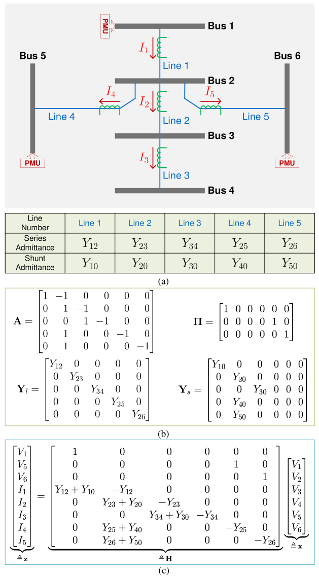
Figure 2: (a) A fictitious six-bus system, where current measurement is represented by an arrow above a current meter. (b) The corresponding $\mathbf{A}$, $\boldsymbol{\Pi}$, $\mathbf{Y}_{l}$, and $\mathbf{Y}_{s}$ for this six-bus system. (c) The full state equation for this six-bus system.

Before explaining the rules for constructing these matrices used in the state equation, a fictitious six-bus system is first presented, as shown in Fig. 2(a). This simple system is used to demonstrate how each of these matrices is constructed for the sake of clarity. As Fig 2(a) indicates, the line current flowing through each line is directly measurable with a current meter. However, bus voltages are measurable only at buses 1, 5, and 6 because of the PMUs are installed only in these three buses. Thus, in this example, the number of buses is $N=6$, the number of PMUs (or the number of buses that have a voltage measurement) is $L=3$, and the number of current measurements is $M=5$.

The explicit rules for constructing each of the four matrices are provided. First, $\mathbf{A}\in\mathbb{R}^{M\times N}$ is the current measurement-bus incidence matrix that indicates the location of the current flow measurements in the network, where the rows and columns of $\mathbf{A}$ represent, respectively, the serial number of the current measurement and the bus number. More specifically, the entries of $\mathbf{A}$ are defined as follows. If the $m$-th current measurement $I_{m}$ (corresponding to the $m$-th row) leaves from the $n$-th bus (corresponding to the $n$-th column) and heads toward the $n^{\prime}$-th bus (corresponding to the $n^{\prime}$-th column), the $(m,n)$-th element of $\mathbf{A}$ is $1$, the $(m,n^{\prime})$-th element of $\mathbf{A}$ is $-1$, and all the remaining entries of $\mathbf{A}$ are identically zero. Second, $\boldsymbol{\Pi}\in\mathbb{R}^{L\times N}$ is the voltage measurement-bus incidence matrix that points out the relationship between a voltage measurement and its corresponding location in the network, where the rows and columns of $\boldsymbol{\Pi}$ represent the serial number of the voltage measurement and the bus number, respectively. Hence, the entries of $\boldsymbol{\Pi}$ can be defined in such a way. If the $l$-th voltage measurement (corresponding to the $l$-th row) is located at the $n$-th bus (corresponding to the $n$-th column), then the $(l,n)$-th element of $\boldsymbol{\Pi}$ is $1$, and all the other elements of $\boldsymbol{\Pi}$ are zero. Third, $\mathbf{Y}_{l}\in\mathbb{C}^{M\times M}$, which denotes the series admittance matrix, is a diagonal matrix, whose diagonal terms are the line admittance of the transmission line being measured. Thus, $\mathbf{Y}_{l}$ is populated using the following single rule. For the $m$-th current measurement, the $(m,m)$-th element of $\mathbf{Y}_{l}$ is the series admittance of the line being measured. Fourth, $\mathbf{Y}_{s}\in\mathbb{C}^{M\times N}$ is the shunt admittance matrix whose elements are determined by the shunt admittances of the lines which have a current measurement. The following rules are used to populate the matrix. If the $m$-th current measurement leaves the $n$-th bus, then the $(m,n)$-th element of $\mathbf{Y}_{s}$ is the shunt admittance of the line, and all the other elements of $\mathbf{Y}_{s}$ are zero. By following these rules, the constructions of $\mathbf{A}$, $\boldsymbol{\Pi}$, $\mathbf{Y}_{l}$, and $\mathbf{Y}_{s}$ for the six-bus system are illustrated in Fig. 2(b).

Given the above definitions, the linear state equation in (4) can be further extended to general linear state equation with $N$ buses, $L$ voltage measurements, denoted by $\mathbf{v}\in\mathbb{C}^{L}$, and $M$ current measurements, denoted by $\mathbf{i}\in\mathbb{C}^{M}$, as follows [18]

$$\underbrace{\begin{bmatrix}\mathbf{v}\\ \mathbf{i}\end{bmatrix}}_{\triangleq\,\mathbf{z}}=\underbrace{\begin{bmatrix}\boldsymbol{\Pi}\\ \mathbf{Y}_{l}\mathbf{A}+\mathbf{Y}_{s}\end{bmatrix}}_{\triangleq\,\mathbf{H}}\mathbf{x},$$ (5)

where $\mathbf{z}\in\mathbb{C}^{L+M}$ denotes a vertical concatenation of the set of voltage and current phasor measurements, $\mathbf{x}\in\mathbb{C}^{N}$ is the complex system state, and ${\bf H}\in\mathbb{C}^{(L+M)\times N}$ is a topology matrix (i.e., also referred to as the measurement matrix in a general linear system).

Considering again the fictitious six-bus system presented earlier, the full system state for this system is also provided in Fig. 2(c) for ease of understanding. Defining $P\triangleq L+M$ and accounting for the measurement error in the linear state equation, (5) then becomes

$$\mathbf{y}=\underbrace{\mathbf{H}\mathbf{x}}_{=\,\mathbf{z}}\,+\,\mathbf{e},$$ (6)

where $\mathbf{y}\in\mathbb{C}^{P}$ is the raw measurement vector of the voltage and current phasors, $\mathbf{z}\in\mathbb{C}^{P}$ is also referred to as the noiseless measurement vector, and $\mathbf{e}\in\mathbb{C}^{P}$ is the measurement error, in which each entry is modeled as an identically and independently distributed (i.i.d.) complex Gaussian random variable with zero mean and variance $\sigma^{2}$.

II-B Data Reduction and Motivation

In reality, all of the measurements must be quantized before being transmitted to the DPCC for processing. For example, modern SCADA systems are equipped with an analog device that converts the measurement into binary values (i.e., the usual word lengths are 12 to 16 bits). To achieve this, the measurements $\mathbf{y}=\left\{y_{\mu}\right\}_{\mu=1}^{P}$ are processed by a complex-valued quantizer in the following componentwise manner:

$$\widetilde{\mathbf{y}}=\left\{\widetilde{y}_{\mu}\right\}_{\mu=1}^{P}=\mathcal{Q}_{\mathbb{C}}\left(\mathbf{y}\right)=\left\{\mathcal{Q}_{\mathbb{C}}\left(y_{\mu}\right)\right\}_{\mu=1}^{P},$$ (7)

where $\widetilde{\mathbf{y}}=\left\{\widetilde{y}_{\mu}\right\}_{\mu=1}^{P}$ is the quantized version of $\mathbf{y}=\left\{y_{\mu}\right\}_{\mu=1}^{P}$, and each complex-valued quantizer $\mathcal{Q}_{\mathbb{C}}\left(\cdot\right)$ is defined as $\widetilde{y}_{\mu}=\mathcal{Q}_{\mathbb{C}}\left(y_{\mu}\right)\triangleq\mathcal{Q}\left(\Re\left(y_{\mu}\right)\right)+\mathrm{j}\mathcal{Q}\left(\Im\left(y_{\mu}\right)\right)$. This means that, for each complex-valued quantizer, two real-valued quantizers exist that separately quantize the real and imaginary part of the measurement data. Here, the real-valued quantizer $\mathcal{Q}\left(\cdot\right)$ is a $B$ bit midrise quantizer [19] that maps a real-valued input to one of $2^{B}$ disjoint quantization regions, which are defined as $\mathscr{R}_{1}=(-\infty,r_{1}],\mathscr{R}_{2}=(r_{1},r_{2}],\ldots,\mathscr{R}_{b}=(r_{b-1},r_{b}],\ldots,\mathscr{R}_{2^{B}}=(r_{2^{B}-1},\infty)$, where $-\infty<r_{1}<r_{2}<\cdots<r_{2^{B}-1}<\infty$. All the regions, except for $\mathscr{R}_{1}$ and $\mathscr{R}_{2^{B}}$, exhibit equal spacing with increments of $\Delta$. In this case, the boundary point of $\mathscr{R}_{b}$ is given by $r_{b}=\left(-2^{B-1}+b\right)\Delta$, for $b=1,\ldots,2^{B}-1$. Thus, if a real-valued input falls in the region $\mathscr{R}_{b}$, then the quantization output is represented by $r_{b}-\frac{\Delta}{2}$, that is, the midpoint of the quantization region in which the input lies.

When the DPCC receives the quantized measurement vector $\widetilde{\mathbf{y}}$, it can perform state estimation using the linear minimum mean square error (LMMSE) method:

$$\widehat{\mathbf{x}}^{\mathsf{LMMSE}}=\left({\bf H}^{\mathsf{H}}{\bf H}+\sigma^{2}\mathbf{I}\right)^{-1}{\bf H}^{\mathsf{H}}\widetilde{\mathbf{y}}.$$ (8)

As can be observed, the accuracy of the LMMSE state estimator highly depends on the quantized measurements $\widetilde{\mathbf{y}}$. A relatively high-resolution quantizer must be employed in the meter device to maintain the high-precision measurement data and therefore prevent the LMMSE performance from being affected by lower-resolution measurements. However, this is unfortunately accompanied by a significant increase in the data for transmission and processing. This unusual trend of increasing data motivates the need for a data-reduction solution.

To reduce the amount of high-precision measurement data, we propose quantizing and representing partial measurements using a very short word length (e.g., 1-6 bits), instead of adopting a higher number of quantization bits to represent all the measurements. In this way, a more efficient use of the available bandwidth can be achieved. However, lower-resolution measurements tend to degrade the state estimation performance. Moreover, quantized measurements with different resolutions require a proper design of the data fusion process to improve the state estimation performance. Given the above problems, we develop in the next section a new framework based on a Bayesian belief inference to incorporate the quantized measurements from the meter devices employing different resolution quantizers to obtain an optimal state estimate.

III State Estimation Algorithm

III-A Theoretical Foundation and Factor Graph Model

The objective of this work is to estimate the system state $\mathbf{x}=\{x_{i}\}_{i=1}^{N}$ from the quantized measurement vector $\widetilde{\mathbf{y}}$ and the knowledge of matrix ${\bf H}$ using the minimum mean square error (MMSE) estimator. A well-known fact is that the Bayesian MMSE inference of $x_{i}$ is equal to the posterior mean, that is,

$$\widehat{x}_{i}^{\mathsf{MMSE}}=\int\,x_{i}\mathscr{P}(x_{i}|{\bf H},\widetilde{\mathbf{y}})\mathrm{d}x_{i},\;\forall i,$$ (9)

where $\mathscr{P}(x_{i}|\mathbf{H},\widetilde{\mathbf{y}})$ is the marginal posterior distribution of the joint posterior distribution $\mathscr{P}(\mathbf{x}|\mathbf{H},\widetilde{\mathbf{y}})$. According to Bayes’ rule, the joint posterior distribution obeys

$$\mathscr{P}(\mathbf{x}|\mathbf{H},\widetilde{\mathbf{y}})\propto\mathscr{P}(\widetilde{\mathbf{y}}|\mathbf{H},\mathbf{x})\mathscr{P}_{\mathsf{o}}(\mathbf{x}),$$ (10)

where $\mathscr{P}(\widetilde{\mathbf{y}}|{\bf H},\mathbf{x})$ is the likelihood function, $\mathscr{P}_{\mathsf{o}}(\mathbf{x})$ is the prior distribution of the system state $\mathbf{x}$, and $\propto$ denotes that the distribution is to be normalized so that it has a unit integral.

Given that the entries of the measurement noise vector ${\bf e}$ are i.i.d. random variables and under the assumption that the prior distribution of $\mathbf{x}$ has a separable form, that is, $\mathscr{P}_{\mathsf{o}}(\mathbf{x})=\prod_{i=1}^{N}\mathscr{P}_{\mathsf{o}}(x_{i})$, (10) can be further factored as

$$\mathscr{P}(\mathbf{x}|\mathbf{H},\widetilde{\mathbf{y}})\propto\prod_{\mu=1}^{P}\mathscr{P}(\widetilde{y}_{\mu}|\mathbf{H},\mathbf{x})\prod_{i=1}^{N}\mathscr{P}_{\mathsf{o}}(x_{i}),$$ (13)

where $\mathscr{P}_{\mathsf{o}}(x_{i})$ is the prior distribution of the $i$-th element of $\mathbf{x}$ and $\mathscr{P}(\widetilde{y}_{\mu}|\mathbf{H},\mathbf{x})$ describes the $\mu$-th measurement with i.i.d. complex Gaussian noise [20], which can be explicitly represented as follows:

$$\mathscr{P}(\widetilde{y}_{\mu}|\mathbf{H},\mathbf{x})=\int_{\widetilde{y}_{\mu}-\frac{\Delta}{2}}^{\widetilde{y}_{\mu}+\frac{\Delta}{2}}\mathscr{N}_{\mathbb{C}}\left(y_{\mu};\sum_{i=1}^{N}H_{\mu i}x_{i},\sigma^{2}\right){\rm d}y_{\mu},$$ (14)

where $H_{\mu i}$ denotes the component of $\mathbf{H}$ in the $\mu$-th row and $i$-th column. For the considered problem, the entries of the system state $\mathbf{x}$ can be treated as i.i.d. complex Gaussian random variables with mean $\nu_{x}$ and variance $\sigma^{2}_{x}$ for each prior distribution $\mathscr{P}_{\mathsf{o}}(x_{i})$, that is, $\mathscr{P}_{\mathsf{o}}(x_{i})=\mathscr{N}_{\mathbb{C}}(\nu_{x},\sigma^{2}_{x})$ [21]. For brevity, the prior distribution of $x_{i}$ is characterized by the prior parameter $\boldsymbol{\theta}_{\mathsf{o}}=\{\nu_{x},\sigma^{2}_{x}\}$.

The decomposition of the joint distribution in (13) can be well represented by a factor graph $\mathcal{G}=(\mathcal{V},\mathcal{F},\mathcal{E})$, where $\mathcal{V}=\{x_{i}\}_{i=1}^{N}$ is the set of unobserved variable nodes, $\mathcal{F}=\{\mathscr{P}(\widetilde{y}_{\mu}|\mathbf{H},\mathbf{x})\}_{\mu=1}^{P}$ is the set of factor nodes, where each factor node ensures (in probability) the condition $\widetilde{y}_{\mu}={\cal Q}_{\mathbb{C}}\left(\sum_{i}H_{\mu i}x_{i}+e_{\mu}\right)$, and $\mathcal{E}$ denotes the set of edges. Specifically, edges indicate the involvement between function nodes and variable nodes; that is, an edge between variable node $x_{i}$ and factor node $\mathscr{P}(\widetilde{y}_{\mu}|\mathbf{H},\mathbf{x})$ indicates that the given factor function $\mathscr{P}(\widetilde{y}_{\mu}|\mathbf{H},\mathbf{x})$ is a function of $x_{i}$. Fig. 3 provides a factor graph representation for the fictitious six buses system shown in Fig. 2.

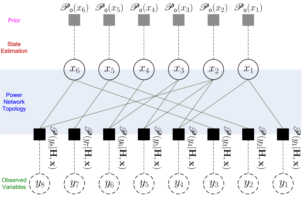
Figure 3: Factor graph representing the state estimation problem for Fig. 2. The unobserved/observed random variables are depicted as solid/dashed lines with open circles, and the factor nodes as depicted as black squares. The factor nodes ensure (in probability) the condition $\widetilde{y}_{\mu}={\cal Q}_{\mathbb{C}}\left(\sum_{i}H_{\mu i}x_{i}+e_{\mu}\right)$.

Given the factor graph representation, message-passing-based algorithms, such as belief propagation (BP) [22, 23], can be applied to compute $\mathscr{P}(x_{i}|\mathbf{H},\widetilde{\mathbf{y}})$ approximately. Methodically, BP passes the following “messages,” which denote the probability distribution functions, along the edges of the graph as follows [24]:

$$\mathscr{M}_{i\rightarrow\mu}^{(t+1)}(x_{i}) \propto\mathscr{P}_{\mathsf{o}}(x_{i})\prod_{\begin{subarray}{c}\gamma\,\in\,\mathscr{L}(i)\\ \gamma\,\neq\,\mu\end{subarray}}\mathscr{M}_{\gamma\rightarrow i}^{(t)}(x_{i}),$$ (15)

$$\mathscr{M}_{\mu\rightarrow i}^{(t+1)}(x_{i}) \propto\!\!\int\!\!\!\!\!\prod_{\begin{subarray}{c}k\,\in\,\mathscr{L}(\mu)\\ k\,\neq\,i\end{subarray}}\!\!\!\!\!\!\mathrm{d}x_{k}\!\Bigg{[}\!\mathscr{P}(\widetilde{y}_{\mu}|\mathbf{H},\mathbf{x})\!\!\!\!\!\prod_{\begin{subarray}{c}k\,\in\,\mathscr{L}(\mu)\\ k\,\neq\,i\end{subarray}}\!\!\!\!\!\!\mathscr{M}_{k\rightarrow\mu}^{(t)}(x_{k})\Bigg{]},\!\!\!$$ (16)

where superscript $t$ indicates the iteration number, $\mathscr{M}_{i\rightarrow\mu}(x_{i})$ is the message from the $i$-th variable node to the $\mu$-th factor node, $\mathscr{M}_{\mu\rightarrow i}(x_{i})$ is the message from the $\mu$-th factor node to the $i$-th variable node, $\mathscr{L}(i)$ is the set of factor nodes that are neighbors of the $i$-th variable node, and $\mathscr{L}(\mu)$ is the set of variable nodes that are neighbors of the $\mu$-th factor node. Then, the approximate marginal distribution is computed according to the following equation:

$$\mathscr{P}^{(t)}(x_{i}|\mathbf{H},\mathbf{y})\propto\mathscr{P}_{\mathsf{o}}(x_{i})\prod_{\mu\,\in\,\mathscr{L}(i)}\mathscr{M}_{\mu\rightarrow i}^{(t)}(x_{i}).$$ (17)

Input: $\widetilde{\mathbf{y}},\mathbf{H},\sigma$

Output: $\{\widehat{x}_{i}^{(t)}\}_{i=1}^{N}$

1 $\widehat{\mathbf{x}}^{\left(0\right)}=\{\widehat{x}_{i}^{\left(0\right)}\}_{i=1}^{N}\leftarrow\{1\}$

2 $\boldsymbol{\tau}^{\left(0\right)}=\{\tau_{i}^{\left(0\right)}\}_{i=1}^{N}\leftarrow\{1\}$

3 $\boldsymbol{\varrho}^{\left(0\right)}=\{{\varrho}_{\mu}^{\left(0\right)}\}_{\mu=1}^{P}\leftarrow\{1\}$

4 $\boldsymbol{\omega}^{\left(0\right)}=\{{\omega}_{\mu}^{\left(0\right)}\}_{\mu=1}^{P}\leftarrow\{\widetilde{y}_{\mu}\}$

5 $t\leftarrow 1$

6 while Stopping criteria are not met do

7       for $\mu=1$ to $P$ do

8             $\varrho^{(t)}_{\mu}\leftarrow\sum_{i=1}^{N}\left|H_{\mu i}\right|^{2}\tau_{i}^{(t-1)}$

9             $\omega_{\mu}^{(t)}\leftarrow\sum_{i=1}^{N}H_{\mu i}\widehat{x}_{i}^{(t-1)}-\frac{\widetilde{y}_{\mu}-\omega_{\mu}^{(t-1)}}{\sigma+\varrho^{(t-1)}_{\mu}}\varrho^{(t)}_{\mu}$

10             $\varsigma_{\mu}^{(t)}\leftarrow\mathbb{VAR}\left[z_{\mu}|\widetilde{y}_{\mu},\omega_{\mu}^{(t)},\varrho_{\mu}^{(t)}\right]$

11             $\widehat{z}_{\mu}^{(t)}\leftarrow\mathbb{E}\left[z_{\mu}|\widetilde{y}_{\mu},\omega_{\mu}^{(t)},\varrho_{\mu}^{(t)}\right]$

12             $\widehat{s}_{\mu}^{(t)}\leftarrow\frac{\widehat{z}_{\mu}^{(t)}-\omega_{\mu}^{(t)}}{\varrho_{\mu}^{(t)}}$

13             $\zeta_{\mu}^{(t)}\leftarrow\left(1-\frac{\varsigma_{\mu}^{(t)}}{\varrho_{\mu}^{(t)}}\right)\frac{1}{\varrho_{\mu}^{(t)}}$

14            

15      $[\ell_{1},\ell_{2},\cdots,\ell_{N}]\leftarrow{\tt permute}(\{1,2,\cdots,N\})$

16       for $k=1$ to $N$ do

17             $i\leftarrow\ell_{k}$

18             $(\Sigma_{i}^{(t)})^{2}\leftarrow\left[\sum_{\mu=1}^{P}\left|H_{\mu i}\right|^{2}\zeta_{\mu}^{(t)}\right]^{-1}$

19             $R_{i}^{(t)}\leftarrow\widehat{x}_{i}^{(t-1)}+(\Sigma_{i}^{(t)})^{2}\sum_{\mu=1}^{P}H_{\mu i}^{*}\,\widehat{s}_{\mu}^{(t)}$

20             $\widehat{x}_{i}^{(t)}\leftarrow\mathbb{E}{\left[x_{i}|\boldsymbol{\theta}_{\mathsf{o}},R_{i}^{(t)},(\Sigma_{i}^{(t)})^{2}\right]}$

21             $\tau_{i}^{(t)}\leftarrow\mathbb{VAR}{\left[x_{i}|\boldsymbol{\theta}_{\mathsf{o}},R_{i}^{(t)},(\Sigma_{i}^{(t)})^{2}\right]}$

22             for $\mu\in\mathscr{L}(i)$  do

23                   $\breve{\varrho}_{\mu}^{(t)}\leftarrow\varrho_{\mu}^{(t)}$

24                   $\varrho_{\mu}^{(t)}\leftarrow\breve{\varrho}_{\mu}^{(t)}+\left|H_{\mu i}\right|^{2}(\tau_{i}^{(t)}-\tau_{i}^{(t-1)})$

25                   $\omega_{\mu}^{(t)}\leftarrow\omega_{\mu}^{(t)}+H_{\mu i}(\widehat{x}_{i}^{(t)}-\widehat{x}_{i}^{(t-1)})-\frac{\widetilde{y}_{\mu}-\omega_{\mu}^{(t-1)}}{\sigma+\varrho^{(t-1)}_{\mu}}(\varrho^{(t)}_{\mu}-\breve{\varrho}_{\mu}^{(t)})$

26            

27      $\nu_{x}\leftarrow\frac{1}{N}\sum_{i=1}^{N}R_{i}^{(t)}$

28       $\sigma_{x}^{2}\leftarrow\frac{1}{N}\sum_{i=1}^{N}\left[(\nu_{x}-R_{i}^{(t)})^{2}+(\Sigma_{i}^{(t)})^{2}\right]$

29      

30      $t\leftarrow t+1$

31

Algorithm 1 EMSwGAMP algorithm

III-B EM-assisted GAMP for the State Estimation Problems

However, according to [25, 26, 13], BP remains computationally intractable for large-scale problems because of the high-dimensional integrals involved and large number of messages required. Moreover, the prior parameters $\boldsymbol{\theta}_{\mathsf{o}}$ and $\sigma^{2}$ are usually unknown in advance. Fortunately, BP can be simplified as the GAMP algorithm [13] based on the central limit theorem and Taylor expansions to enhance computational tractability. By contrast, the EM algorithm can be applied to learn the prior parameters [16]. With the aid of these two algorithms, we develop an iterative method involving the following two phases per iteration for the state estimation problems: First, “swept” GAMP (SwGAMP) [15], a modified version of GAMP, is exploited to estimate $\mathbf{x}$. Second, the EM algorithm is applied to learn the prior parameters from the data at hand. The stepwise implementation procedure of the proposed state estimation scheme, referred to as EMSwGAMP, is presented in Algorithm 1. Considering the space limitations, a detailed derivation of (complex) GAMP and EM is excluded in this paper. For the details, refer to [13, 14, 15, 27, 16]. Then, we provide several explanations for each line of Algorithm 1 to ensure better understanding of the proposed scheme.

In Algorithm 1, $\widehat{x}_{i}^{(t)}$ denotes the estimate of the $i$-th element of $\mathbf{x}$ in the $t$-th iteration and $\tau_{i}^{(t)}$ can be interpreted as an approximation of the posterior variance of $\widehat{x}_{i}^{(t)}$; these two quantities are initialized as $\widehat{x}_{i}^{(0)}=1$ and $\tau_{i}^{(0)}=1$, respectively. For each factor node, we introduce two auxiliary variables $\omega_{\mu}^{(t)}$ and $\varrho_{\mu}^{(t)}$, given in Lines 9 and 8 of Algorithm 1, describing the current mean and variance estimates of the $\mu$-th element of $\widetilde{\mathbf{y}}$, respectively. The initial conditions of $\omega_{\mu}^{(0)}$ and $\varrho_{\mu}^{(0)}$ are specified in Lines 4 and 3 of Algorithm 1, respectively. As stated previously, $z_{\mu}$ is the $\mu$-th element of the noise free measurement vector $\mathbf{z}$, that is, $z_{\mu}=\sum_{i}H_{\mu i}\,x_{i}$. Therefore, according to the derivations of [13], $z_{\mu}$ conditioned on $x_{i}$ can be further approximated as a Gaussian distribution with the mean and variance given in Lines 9 and 8 of Algorithm 1, respectively, which are evaluated with respect to the following expression

$$\mathscr{P}(z_{\mu}|\widetilde{y}_{\mu})\propto\int_{\widetilde{y}_{\mu}-\frac{\Delta}{2}}^{\widetilde{y}_{\mu}+\frac{\Delta}{2}}\mathscr{N}_{\mathbb{C}}(y_{\mu};z_{\mu},\sigma^{2})\mathscr{N}_{\mathbb{C}}(z_{\mu};\omega_{\mu}^{(t)},\varrho_{\mu}^{(t)}){\rm d}y_{\mu}.$$ (18)

(18) represents the quantization noise that can be regarded as a Gaussian distribution whose mean is $\omega_{\mu}$ and variance is $\varrho_{\mu}$. Finally, the messages from factor nodes to variable nodes are reduced to a simple message, which is parameterized by $\widehat{s}_{\mu}$ and $\zeta_{\mu}$, given in Lines 12 and 13 of Algorithm 1. Therefore, we refer to messages $\{\widehat{s}_{\mu},\zeta_{\mu}\}$ as measurement updates.

Similarly, for the variable nodes, we also introduce two auxiliary variables $R_{i}^{(t)}$ and $(\Sigma_{i}^{(t)})^{2}$, given in Lines 18 and 17 of Algorithm 1, describing the current mean and variance estimates of the $i$-th element of $\mathbf{x}$ without considering the prior information of $x_{i}$, respectively. Then, adding the prior information of $x_{i}$, that is, $\mathscr{P}_{\mathsf{o}}(x_{i})=\mathscr{N}_{\mathbb{C}}(\nu_{x},\sigma^{2}_{x})$, to the message updates, the posterior mean and variance of $x_{i}$ are given in Lines 19 and 20 of Algorithm 1, respectively where is considered with respect to the following expression:

$$\!\mathscr{P}(x_{i};\widehat{x}_{i}^{(t)},\tau_{i}^{(t)})\!\propto\!\mathscr{N}_{\mathbb{C}}(x_{i};\nu_{x},\sigma^{2}_{x})\mathscr{N}_{\mathbb{C}}(x_{i};R_{i}^{(t)},(\Sigma_{i}^{(t)})^{2}).\!$$ (19)

Here, $\widehat{x}_{i}^{(t)}$ (i.e., the calculation of Expectation in Line 19 of Algorithm 1) and $\tau_{i}^{(t)}$ (i.e., the calculation of VAR in Line 20 of Algorithm 1) can be easily obtained using the standard formulas for Gaussian distributions as [28, 29]

$$\widehat{x}_{i}^{(t)} =R_{i}^{(t)}+\frac{(\Sigma_{i}^{(t)})^{2}}{(\Sigma_{i}^{(t)})^{2}+\sigma^{2}_{x}}{\left(\nu_{x}-R_{i}^{(t)}\right)},$$ (20)

$$\tau_{i}^{(t)} =\frac{(\Sigma_{i}^{(t)})^{2}\sigma^{2}_{x}}{(\Sigma_{i}^{(t)})^{2}+\sigma^{2}_{x}}.$$ (21)

Manoel et al. [15] slightly modified the update scheme for GAMP, where partial quantities are updated sequentially rather than in parallel, to improve the stability of GAMP. Specifically, $\sum_{i}H_{\mu i}\widehat{x}_{i}^{(t-1)}$ and $\varrho_{\mu}^{(t)}$ are recomputed as the sweep updates over $i$ for a single iteration step. Lines 22-24 of Algorithm 1 are the core steps to perform the so-called sweep (or reordering) updates. In brief, we refer to messages $\{\widehat{x}_{i},\tau_{i}\}$ as variable updates and to messages $\{\widehat{s}_{\mu},\zeta_{\mu}\}$ as measurement updates for the SwGAMP algorithm. One iteration of the SwGAMP algorithm involves the implementation of these updates together with the estimation of the system state $\mathbf{x}$.

In the first phase of Algorithm 1, the prior parameters $\boldsymbol{\theta}_{\mathsf{o}}=\{\nu_{x},\sigma^{2}_{x}\}$ are treated as known parameters, but may be unknown in practice. Thus, the second phase of the proposed algorithm is to adopt the EM algorithm to learn the prior parameters $\boldsymbol{\theta}_{\mathsf{o}}$ on the basis of the quantities acquired in the first phase of the algorithm. The EM algorithm is a general iterative method for likelihood optimization in probabilistic models with hidden variables. In our case, the EM-updates will be expressed in the following form [16]

$$\boldsymbol{\theta}_{\mathsf{o}}^{\rm new}=\operatornamewithlimits{arg\,max}_{\boldsymbol{\theta}_{\mathsf{o}}}\mathbb{E}\left\{\ln\mathscr{P}(\mathbf{x},\mathbf{y};\boldsymbol{\theta}_{\mathsf{o}})\right\},$$ (22)

where the expectation takes over the posterior probability of $\mathbf{x}$ conditioned on $\boldsymbol{\theta}_{\mathsf{o}}$ and $\mathbf{y}$. Following similar steps in [16], we can derive a set of EM-based update equations for the hyperparameters, that is, the prior information of the system states (i.e., $\nu_{x}$ and $\sigma^{2}_{x}$) that should be inferred. The detailed EM updates for the hyperparameters are provided in Lines 25 and 26 of Algorithm 1, respectively. Notably, the quantities $\{R_{i}^{(t)}\}_{i=1}^{N}$, $\{(\Sigma_{i}^{(t)})^{2}\}_{i=1}^{N}$, $\{\widehat{z}_{\mu}^{(t)}\}_{\mu=1}^{P}$, and $\{\varsigma_{\mu}^{(t)}\}_{\mu=1}^{P}$ are readily available after running the SwGAMP algorithm in the first phase.

Remark 3.1 (Calculating Lines 10 and 11 of Algorithm 1 with high resolution representation of the measured data) : In modern SCADA systems, each measurement is quantized and represented using a word length of 12 (or 16) bits. With such high precision representation of the measurement data, the error between the quantized value $\widetilde{y}_{\mu}$ and the actual value $y_{\mu}$ can be negligible, that is, $\widetilde{y}_{\mu}\simeq{y}_{\mu}$. In this case, (18) can be rewritten as follows:

$$\mathscr{P}(z_{\mu}|\widetilde{y}_{\mu})\propto\mathscr{N}_{\mathbb{C}}(y_{\mu};z_{\mu},\sigma^{2})\mathscr{N}_{\mathbb{C}}(z_{\mu};\omega_{\mu}^{(t)},\varrho_{\mu}^{(t)}).$$ (23)

Then, the moments, $\widehat{z}_{\mu}^{(t)}$ and $\varsigma_{\mu}^{(t)}$, can be easily obtained using standard formulas for Gaussian distributions, as follows [28]:

$$\widehat{z}_{\mu}^{(t)} =\omega_{\mu}^{(t)}+\frac{\varrho_{\mu}^{(t)}}{\varrho_{\mu}^{(t)}+\sigma^{2}}{\left(\widetilde{y}_{\mu}-\omega_{\mu}^{(t)}\right)},$$ (24)

$$\varsigma_{\mu}^{(t)} =\frac{\varrho_{\mu}^{(t)}\sigma^{2}}{\varrho_{\mu}^{(t)}+\sigma^{2}}.\vspace{-.05in}$$ (25)

Remark 3.2 (Calculating Lines 10 and 11 of Algorithm 1 under the “quantized” scenario) : When quantization error is nonnegligible, particularly at coarse quantization levels, (23) is no longer valid because of the fact that using $\widetilde{y}_{\mu}$ to approximate ${y}_{\mu}$ will result in severe performance degradation. In this case, we have to adopt (18) to determine the conditional mean $\widehat{z}_{\mu}^{(t)}$ and conditional variance $\varsigma_{\mu}^{(t)}$, which can be obtained as follows:

$$\widehat{z}_{\mu}^{(t)} =\frac{\int_{\widetilde{y}_{\mu}-\frac{\Delta}{2}}^{\widetilde{y}_{\mu}+\frac{\Delta}{2}}y_{\mu}\mathscr{N}_{\mathbb{C}}(y_{\mu};\omega_{\mu}^{(t)},\sigma^{2}+\varrho_{\mu}^{(t)}){\rm d}y_{\mu}}{\int_{\widetilde{y}_{\mu}-\frac{\Delta}{2}}^{\widetilde{y}_{\mu}+\frac{\Delta}{2}}\mathscr{N}_{\mathbb{C}}(y_{\mu};\omega_{\mu}^{(t)},\sigma^{2}+\varrho_{\mu}^{(t)}){\rm d}y_{\mu}},$$ (26)

$$\varsigma_{\mu}^{(t)} =\frac{\int_{\widetilde{y}_{\mu}-\frac{\Delta}{2}}^{\widetilde{y}_{\mu}+\frac{\Delta}{2}}|y_{\mu}-\widehat{y}_{\mu}^{(t)}|^{2}\mathscr{N}_{\mathbb{C}}(y_{\mu};\omega_{\mu}^{(t)},\sigma^{2}+\varrho_{\mu}^{(t)}){\rm d}y_{\mu}}{\int_{\widetilde{y}_{\mu}-\frac{\Delta}{2}}^{\widetilde{y}_{\mu}+\frac{\Delta}{2}}\mathscr{N}_{\mathbb{C}}(y_{\mu};\omega_{\mu}^{(t)},\sigma^{2}+\varrho_{\mu}^{(t)}){\rm d}y_{\mu}}.$$ (27)

Explicit expressions of (26) and (27) are provided in [20].

Remark 3.3 (Stopping criteria): The algorithm can be discontinued either when a predefined number of iterations is reached or when it converges in the relative difference of the norm of the estimate of $\mathbf{x}$, or both. The relative difference of the norm is given by the quantity $\epsilon\triangleq\sum_{i}^{N}|\widehat{x}_{i}^{(t)}-\widehat{x}_{i}^{(t-1)}|^{2}$.

IV Simulation Results and Discussion

In this section, we evaluate the performance of the proposed EMSwGAMP algorithm for single-phase state and three-phase state estimations. The optimal PMU placement issue is not included in this study, and we assume that PMUs are placed in terminal buses. In the single-phase state estimation, IEEE 69-bus radial distribution network [30] is used for the test system, where the subset of buses with PMU measurements is denoted by $\mathcal{P}_{69}=\{1,27,35,46,50,52,67,69\}$. A modified version of IEEE $69$-bus radial distribution network, referred to as 69m in this study, is examined to verify the robustness of the proposed algorithm. The system settings of this modified test system are identical to those of the IEEE 69-bus radial distribution network, with the exception of the bus voltages of this test system being able to vary within a large range, thereby increasing the load levels of this system. For these two test system, we have $68$ current measurements and $8$ voltage measurements. The software toolbox MATPOWER [31] is utilized to run the proposed state estimation algorithm for various cases in the single-phase state estimation. The IEEE 37-bus three-phase system is used as the test system for the three-phase state estimation, where the subset of buses with PMU measurements is denoted by $\mathcal{P}_{37}=\{1,10,15,20,29,35\}$. In contrast to the single-phase state estimation, the system state of the three-phase estimation is generated by test system documents instead of MATPOWER. We have $105$ current measurements and $18$ voltage measurements in 37-bus three-phase system. Prior distributions of the voltage at each bus for different test systems can be found in Table I. In each estimation, the mean squared error (MSE) of the bus voltage magnitude and that of the bus voltage phase angle are used as comparison measures, which are expressed as ${\rm MSE}=\frac{1}{N}\sum_{i=1}^{N}|x_{i}-\widehat{x}_{i}|^{2}$, ${\rm MSE}_{\rm magn}=\frac{1}{N}\sum_{i=1}^{N}(|x_{i}|-|\widehat{x}_{i}|)^{2}$, and ${\rm MSE}_{\rm phase}=\frac{1}{N}\sum_{i=1}^{N}[\arg(x_{i})-\arg(\widehat{x}_{i})]^{2}$, respectively. The LMMSE estimator is tested for comparison. In our implementation, termination of Algorithm 1 is declared when the corresponding constraint violation is less than $\epsilon=10^{-8}$. A total of $1,000$ Monte Carlo simulations were conducted and evaluated to obtain average results and to analyze the achieved measures. The simulations for computation time were conducted utilizing an Intel i7-4790 computer with 3.6 GHz CPU and 16 GB RAM. For clarity, the number of measurements quantized to be $\mathcal{B}$-bit is denoted as $\mathcal{K}$, where $\mathcal{B}$ denotes the number of bits used for quantization.

TABLE I: The prior distribution of bus voltage for different systems

	$N$	Magnitude	Phase	$\sigma^{2}_{x}$
		(mean)	(mean)
single-phase	69m	$1.00$	$5.60\times 10^{-4}$	$5.46\times 10^{-7}$
	69m	$1.04$	$1.71\times 10^{-2}$	$5.66\times 10^{-4}$
three-phase	37m	$0.01$	$1.12$	$9.86\times 10^{-1}$

TABLE II: Average estimation results obtained by EMSwGAMP and LMMSE with the unquantized measured data for the various systems

$N$	Algorithm	${\rm MSE}$	${\rm MSE}_{\rm magn}$	${\rm MSE}_{\rm phase}$
69m	EMSwGAMP	$3.84\times 10^{-4}$	$2.06\times 10^{-4}$	$7.78\times 10^{-4}$
	LMMSE	$8.16\times 10^{-4}$	$4.65\times 10^{-4}$	$3.55\times 10^{-4}$
69m	EMSwGAMP	$7.11\times 10^{-4}$	$3.00\times 10^{-4}$	$3.78\times 10^{-4}$
	LMMSE	$8.22\times 10^{-4}$	$4.75\times 10^{-4}$	$3.23\times 10^{-4}$

Table II shows a summary of the average ${\rm MSE}$, ${\rm MSE}_{\rm magn}$, and ${\rm MSE}_{\rm phase}$ achieved by EMSwGAMP and LMMSE for single-phase state estimation with various systems. The results show that even under the traditional unquantized setting, EMSwGAMP still outperforms LMMSE because EMSwGAMP exploits the statistical knowledge of the estimated parameters $\boldsymbol{\theta}_{\mathsf{o}}$, which is learned from the data via the second phase of EMSwGAMP, that is, the EM learning algorithm. Table III reveals that the estimation results of the system states using EMSwGAMP are close to the true values, which validates the effectiveness of the proposed learning algorithm. From a detailed inspection of Table III, we found that the mean value of voltage magnitude can be exactly estimated through the EM learning algorithm. Therefore, the average ${\rm MSE}_{\rm magn}$ of EMSwGAMP is better than that of LMMSE. However, the mean value of voltage phase cannot be estimated accurately by the EM learning algorithm. As a result, the average ${\rm MSE}_{\rm phase}$ of EMSwGAMP is inferior to that of LMMSE.

TABLE III: Parameter learning results using EMSwGAMP

$N$	Algorithm	Magnitude	Phase
		(mean)	(mean)
69m	True value	$1.00$	$\phantom{-}5.60\times 10^{-4}$
	EMSwGAMP	$1.00$	$-2.53\times 10^{-4}$
69m	True value	$1.04$	$\phantom{-}1.71\times 10^{-2}$
	EMSwGAMP	$1.04$	$\phantom{-}1.10\times 10^{-2}$

We consider an extreme scenario where several measurements are quantized to “$1$” bit, but others are not, to reduce the amount of transmitted data. The measurements selected to be quentized are provided in Appendix A. Table IV shows the average ${\rm MSE}$, ${\rm MSE}_{\rm magn}$, and ${\rm MSE}_{\rm phase}$ against $\mathcal{K}$ obtained by EMSwGAMP, where in the performance of the LMMSE algorithm with $\mathcal{K}=17$ is also included for the purpose of comparison. The following observations are noted on the basis of Table IV: First, when the measurement is quantized with 1 bit, we only know that the measurement is positive or not so that the information related to the system is lost. Hence, as expected, increasing $\mathcal{K}$ naturally degrades the average MSE performance because more information is lost. However, the achieved performance of the 69-bus test system is less sensitive to $\mathcal{K}$ because the bus voltage variations in this system are small. Thus, the proposed algorithm can easily deal with incomplete data. Second, for the system with large bus voltage fluctuations, the obtained ${\rm MSE}_{\rm phase}$ performance of the modified 69-bus test system can still achieve $10^{-3}$ when $\mathcal{K}\leq 17$. However, with $\mathcal{K}=17$, the LMMSE algorithm exhibits poor performance for both considered test systems, which cannot be used in practice.

TABLE IV: Average estimation results obtained by EMSwGAMP with different number of $1$-bit quantized measurements for the various systems

$N$	Algorithm	$\mathcal{K}$	${\rm MSE}$	${\rm MSE}_{\rm magn}$	${\rm MSE}_{\rm phase}$
69m	EMSwGAMP	$\phantom{0}0$	$3.84\times 10^{-4}$	$2.07\times 10^{-4}$	$1.77\times 10^{-4}$
		$\phantom{0}2$	$1.00\times 10^{-3}$	$5.97\times 10^{-4}$	$4.44\times 10^{-4}$
		$\phantom{0}4$	$1.00\times 10^{-3}$	$6.18\times 10^{-4}$	$4.74\times 10^{-4}$
		$17$	$1.00\times 10^{-3}$	$5.76\times 10^{-4}$	$4.19\times 10^{-4}$
		$19$	$1.00\times 10^{-3}$	$5.72\times 10^{-4}$	$4.34\times 10^{-4}$
		$23$	$1.00\times 10^{-3}$	$5.89\times 10^{-4}$	$4.56\times 10^{-4}$
		$27$	$1.10\times 10^{-3}$	$6.04\times 10^{-4}$	$4.87\times 10^{-4}$
		$34$	$1.00\times 10^{-3}$	$5.70\times 10^{-4}$	$4.47\times 10^{-4}$
		$42$	$1.00\times 10^{-3}$	$5.59\times 10^{-4}$	$4.41\times 10^{-4}$
	LMMSE	$17$	$2.39\times 10^{-1}$	$1.07\times 10^{-1}$	$1.59\times 10^{-1}$
69m	EMSwGAMP	$\phantom{0}0$	$7.00\times 10^{-4}$	$3.90\times 10^{-4}$	$3.58\times 10^{-4}$
		$\phantom{0}2$	$1.00\times 10^{-3}$	$5.59\times 10^{-4}$	$3.87\times 10^{-4}$
		$\phantom{0}4$	$1.00\times 10^{-3}$	$5.68\times 10^{-4}$	$3.99\times 10^{-4}$
		$17$	$1.00\times 10^{-3}$	$5.40\times 10^{-4}$	$3.74\times 10^{-4}$
		$19$	$1.20\times 10^{-3}$	$7.19\times 10^{-4}$	$4.37\times 10^{-4}$
		$23$	$1.20\times 10^{-3}$	$7.12\times 10^{-4}$	$4.64\times 10^{-4}$
		$27$	$1.30\times 10^{-3}$	$7.20\times 10^{-3}$	$5.17\times 10^{-4}$
		$34$	$1.30\times 10^{-3}$	$7.45\times 10^{-3}$	$5.44\times 10^{-4}$
		$42$	$1.50\times 10^{-3}$	$8.00\times 10^{-3}$	$6.04\times 10^{-4}$
	LMMSE	$17$	$2.46\times 10^{-1}$	$1.01\times 10^{-1}$	$1.65\times 10^{-1}$

Table IV also shows that the proposed algorithm can only achieve reasonable performance with $\mathcal{K}=17$. This finding naturally raises the question: How many quantization bits of these $17$ measurements are needed to achieve a performance close to that of the unquantized measurements? Therefore, Table V shows the performance of the proposed algorithm using different quantization bits for the $17$ measurements, where the number of bits used for quantization is denoted as $\mathcal{B}$. For ease of reference, the performance of the proposed algorithm with the unquantized measurements is also provided. Furthermore, the average running time of the proposed algorithm for Table V is provided in Table VI. Table V shows that increasing $\mathcal{B}$ results in the improvement of the state estimation performance. However, as shown in Table VI, the required running time also increases with the value of $\mathcal{B}$. Fortunately, the required running time is within 2 s even at $\mathcal{B}=6$. Moreover, if we further increase the quantization bit from $\mathcal{B}=6$ to $\mathcal{B}=7$, the performance remains the same. However, the corresponding running time rapidly increases from 1.90 s to 2.45 s. These findings indicate that $(\mathcal{B},\mathcal{K})=(6,17)$ are appropriate parameters for the proposed framework. Therefore, in the following simulations, we consider the scenario where more than half of the measurements are quantized to $6$ bits and the others are unquantized to reduce the data transmitted from the measuring devices to the data gathering center further.

TABLE V: The performance of EMSwGAMP using different quantization bits for the $17$ measurements for the various systems

$N$	$\mathcal{B}$-bit	${\rm MSE}$	${\rm MSE}_{\rm magn}$	${\rm MSE}_{\rm phase}$
69m	1-bit	$9.49\times 10^{-4}$	$5.40\times 10^{-4}$	$4.05\times 10^{-4}$
	2-bit	$9.49\times 10^{-4}$	$5.40\times 10^{-4}$	$4.05\times 10^{-4}$
	3-bit	$9.47\times 10^{-4}$	$5.39\times 10^{-4}$	$4.04\times 10^{-4}$
	4-bit	$9.11\times 10^{-4}$	$5.22\times 10^{-4}$	$3.87\times 10^{-4}$
	5-bit	$8.80\times 10^{-4}$	$5.06\times 10^{-4}$	$3.71\times 10^{-4}$
	6-bit	$8.69\times 10^{-4}$	$5.00\times 10^{-4}$	$3.66\times 10^{-4}$
	unquantized	$3.78\times 10^{-4}$	$2.02\times 10^{-4}$	$1.75\times 10^{-4}$
69m	1-bit	$9.79\times 10^{-4}$	$5.53\times 10^{-4}$	$3.91\times 10^{-4}$
	2-bit	$9.79\times 10^{-4}$	$5.53\times 10^{-4}$	$3.91\times 10^{-4}$
	3-bit	$9.75\times 10^{-4}$	$5.49\times 10^{-4}$	$3.89\times 10^{-4}$
	4-bit	$9.36\times 10^{-4}$	$5.28\times 10^{-4}$	$3.73\times 10^{-4}$
	5-bit	$9.04\times 10^{-4}$	$5.12\times 10^{-4}$	$3.58\times 10^{-4}$
	6-bit	$8.93\times 10^{-4}$	$5.06\times 10^{-4}$	$3.54\times 10^{-4}$
	unquantized	$7.15\times 10^{-4}$	$3.09\times 10^{-4}$	$3.74\times 10^{-4}$

TABLE VI: The run time of EMSwGAMP using different quantization bits for the $17$ measurements for the various systems

$N$	$\mathcal{B}$-bit	Time (s)		$N$	$\mathcal{B}$-bit	Time (s)
69m	1-bit	$1.22$		69m	1-bit	$1.17$
	2-bit	$1.28$			2-bit	$1.23$
	3-bit	$1.31$			3-bit	$1.29$
	4-bit	$1.37$			4-bit	$1.36$
	5-bit	$1.56$			5-bit	$1.53$
	6-bit	$1.90$			6-bit	$1.87$
	unquantized	$0.20$			unquantized	$0.20$

Table VII shows the average performance of two algorithms with $\mathcal{K}=34$ and $\mathcal{K}=42$ for the two test systems. Here, $\mathcal{K}$ denotes the number of 6-bit quantized measurements and the performance of EMSwGAMP using only the unquantized measurements is also listed for convenient reference. Notably, the proposed EMSwGAMP algorithm significantly outperforms LMMSE, where the performance of LMMSE deteriorates again to an unacceptable level. We also observed that increasing the number of $6$ bit quantized measurements from $\mathcal{K}=34$ to $\mathcal{K}=42$ only results in a slight performance degradation for EMSwGAMP. Consequently, by using EMSwGAMP, we can drastically reduce the amount of transmitted data without compromising performance. The total amount of measurements of a 69-bus test system is $76$, where $68$ current measurements and 8 voltage measurements originate from the meters and PMUs, respectively. Therefore, if the measurements are quantized as $16$ bits for the conventional meters and PMUs, $16\times 76=1,216$ bits should be transmitted. However, for the proposed algorithm with $\mathcal{K}=34$ (i.e., 34 measurements quantized with 6 bits and 42 measurements quantized with 16 bits), only $34\times 6+42\times 16=876$ bits should be transmitted. In this case, the transmission data can be reduced by $27.96\%$. Similarly, for the proposed algorithm with $\mathcal{K}=42$ (i.e., 42 measurements quantized with 6 bits and 34 measurements quantized with 16 bits), the transmission data can be reduced by $34.53\%$. In addition, we further discuss the required transmission bandwidth of the proposed framework and the conventional system under the assumption that the meters can update measurements every 1 s. As defined by IEEE 802.11n, when the data are modulated with quadrature phase-shift keying for a 20 MHz channel bandwidth, the data rate is $21.7$ Mbps. Therefore, we can approximate the transmission rate as 1.085/Hz/s. For the proposed algorithm with $\mathcal{K}=34$ and $\mathcal{B}=6$ (i.e., $876$ bits should be transmitted), the required transmission bandwidth is $808$ Hz. However, the required transmission bandwidth for the conventional system (i.e., $1,216$ bits should be transmitted) is $1,121$ Hz. In this case, the proposed architecture can also reduce the transmission bandwidth by $27.83\%$. Notably, this study only focuses on the reduction of the transmission data. However, references that specifically discuss the smart meter data transmission system are few (e.g., [32, 33]), which are not considered in this study. Further studies can expand the scope of the present work to include these transmission mechanism to provide more efficient transmission framework.

TABLE VII: Average estimation results obtained by EMSwGAMP and LMMSE with different numbers of $6$-bit quantized measurements for the various systems

$N$	$\mathcal{K}$	Algorithm	${\rm MSE}$	${\rm MSE}_{\rm magn}$	${\rm MSE}_{\rm phase}$
69m	34	unquantized	$3.86\times 10^{-4}$	$2.11\times 10^{-4}$	$1.78\times 10^{-4}$
		EMSwGAMP	$1.00\times 10^{-3}$	$6.01\times 10^{-4}$	$4.34\times 10^{-4}$
		LMMSE	$9.39\times 10^{-1}$	$9.34\times 10^{-1}$	$2.21\times 10^{-1}$
	42	unquantized	$3.77\times 10^{-4}$	$2.06\times 10^{-4}$	$1.72\times 10^{-4}$
		EMSwGAMP	$7.89\times 10^{-4}$	$4.52\times 10^{-4}$	$3.32\times 10^{-4}$
		LMMSE	$9.39\times 10^{-1}$	$9.32\times 10^{-1}$	$2.88\times 10^{-1}$
69m	34	unquantized	$7.78\times 10^{-4}$	$3.89\times 10^{-4}$	$3.56\times 10^{-4}$
		EMSwGAMP	$1.10\times 10^{-3}$	$6.28\times 10^{-4}$	$4.31\times 10^{-4}$
		LMMSE	$1.02$	$1.02$	$2.10\times 10^{-1}$
	42	unquantized	$6.77\times 10^{-4}$	$2.86\times 10^{-4}$	$3.59\times 10^{-4}$
		EMSwGAMP	$1.20\times 10^{-3}$	$6.56\times 10^{-4}$	$4.53\times 10^{-4}$
		LMMSE	$1.02$	$1.02$	$2.69\times 10^{-1}$

Finally, we evaluate the performance of the proposed EMSwGAMP algorithm for three-phase state estimation. The above simulation results show that almost half of the measurements can be represented with low-precision. Hence, in this test system, $\mathcal{K}=51$ measurements are quantized with 6-bit. Therefore, Table VIII shows the average performance of two algorithms with $\mathcal{K}=51$ for IEEE 37-bus three-phase system. The performance of EMSwGAMP using only unquantized measurements is also included for ease of reference. Table VIII shows that EMSwGAMP still outperformed LMMSE but only with a slight degradation as compared to the unquantized result. The proposed EMSwGAMP algorithm can reduce transmission data by $25.91\%$ compared to the high-precision measurement data. Hence, the proposed algorithm can be applied not only to a single-phase but also to a three-phase system. Most importantly, the proposed algorithm can also decrease the amount of data required to be transmitted and processed.

TABLE VIII: Average estimation results obtained through EMSwGAMP and LMMSE with $6$-bit quantized measurements for the three-phase systems

$N$	$\mathcal{K}$	Algorithm	${\rm MSE}$	${\rm MSE}_{\rm magn}$	${\rm MSE}_{\rm phase}$
37	51	unquantized	$2.02\times 10^{-4}$	$1.17\times 10^{-4}$	$8.79\times 10^{-5}$
		EMSwGAMP	$6.64\times 10^{-4}$	$4.42\times 10^{-4}$	$2.30\times 10^{-4}$
		LMMSE	$0.92$	$0.92$	$1.49\times 10^{-4}$

V Conclusion

We first proposed a data reduction technique via coarse quantization of partial uncensored measurements and then developed a new framework based on a Bayesian belief inference to incorporate quantization-caused measurements of different qualities to obtain an optimal state estimation and reduce the amount of data while still incorporating different quality of data. The simulation results indicated that the proposed algorithm performs significantly better than other linear estimates, even for a case scenario in which more than half of measurements are quantized to $6$ bits. This finding verifies the effectiveness of the proposed scheme.

Appendix A How the measurements are being picked for quantization

For ease of explanation, a 69-bus test system is provided in Fig. 4, where the subset of buses $\mathcal{M}=\{1,2,\ldots,27\}$, called the main chain of the system, plays an important role for estimating the system states. Therefore, the measurements from the side chain of the system are selected for quantization. In addition, the numbers of the quantized measurements considered in this study are $\mathcal{K}=2$, $\mathcal{K}=4$, $\mathcal{K}=17$, $\mathcal{K}=19$, $\mathcal{K}=23$, $\mathcal{K}=27$, $\mathcal{K}=34$, and $\mathcal{K}=42$. More specifically, if $\mathcal{K}=2$, the current measurements from the subset of buses $\{12,68,69\}$ are selected for quantization; if $\mathcal{K}=4$, the current measurements from the subset of buses $\{12,68,69\}$ and $\{11,66,67\}$ are selected for quantization; if $\mathcal{K}=17$, the current measurements from the subset of buses $\{12,68,69\}$, $\{11,66,67\}$ and $\{9,53,54,\ldots,65\}$ are being picked for quantization; if $\mathcal{K}=19$, the current measurements from the subset of buses $\{12,68,69\}$, $\{11,66,67\}$, $\{8,51,52\}$ and $\{9,53,54,\ldots,65\}$ are selected for quantization; if $\mathcal{K}=23$, the current measurements from the subset of buses $\{12,68,69\}$, $\{11,66,67\}$, $\{8,51,52\}$, $\{4,47,48,49,50\}$, and $\{9,53,54,\ldots,65\}$ are selected for quantization; if $\mathcal{K}=27$, the current measurements from the subset of buses $\{12,68,69\}$, $\{11,66,67\}$, $\{8,51,52\}$, $\{3,28,29,\ldots,35\}$, and $\{9,53,54,\ldots,65\}$ are selected for quantization; if $\mathcal{K}=34$, the current measurements from the subset of buses $\{12,68,69\}$, $\{11,66,67\}$, $\{8,51,52\}$, $\{4,47,48,49,50\}$, $\{36,38,\ldots,46\}$, and $\{9,53,54,\ldots,65\}$ are selected for quantization; if $\mathcal{K}=42$, the current measurements from the subset of buses $\{12,68,69\}$, $\{11,66,67\}$, $\{8,51,52\}$, $\{4,47,48,49,50\}$, $\{3,28,29,\ldots,35\}$, $\{36,38,\ldots,46\}$, and $\{9,53,54,\ldots,65\}$ are selected for quantization.

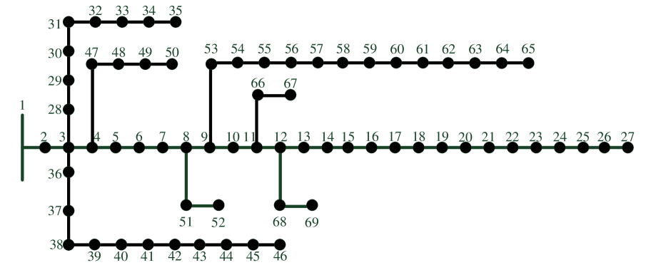
Figure 4: A 69-bus test system.

References

- [1] “The smart grid: An introduction,” prepared by Litos Strategic Communication for U.S. Department of Energy, Tech. Rep., Oct. 2008.
- [2] Y.-F. Huang, S. Werner, J. Huang, N. Kashyap, and V. Gupta, “State estimation in electric power grids: meeting new challenges presented by the requirements of the future grid,” IEEE Signal Process. Mag., vol. 29, no. 5, pp. 33–43, Sep. 2012.
- [3] K. Nagasawa, C. R. Upshaw, J. D. Rhodes, C. L. Holcomb, D. A. Walling, and M. E. Webber, “Data management for a large-scale smart grid demonstration project in Austin, Texas,” in Proc. ASME Int. Conf. Energy Sustainability, San Diego, CA, Jul. 2012, pp. 1027–1031.
- [4] A. Abur and A. G. Exposito, Power System State Estimation: Theory and Implementation. Boca Raton, FL: CRC Press, 2004.
- [5] X. Li, A. Scaglione, and T. H. Chang, “A framework for phasor measurement placement in hybrid state estimation via gauss」newton,” IEEE Trans. Power Syst., vol. 29, no. 2, pp. 824–832, Mar. 2014.
- [6] M. Göl and A. Abur, “LAV based robust state estimation for systems measured by PMUs,” IEEE Trans. Smart Grid, vol. 5, no. 4, pp. 1808–1814, Jul. 2014.
- [7] M. Hurtgen and J.-C. Maun, “Advantages of power system state estimation using phasor measurement units,” in Proc. Power Syst. Comput. Conf., Glasgow, Scotland, Jul. 2008, pp. 1–7.
- [8] A. G. Phadke, J. S. Thorp, R. F. Nuqui, and M. Zhou, “Recent developments in state estimation with phasor measurements,” in Proc. IEEE Power Syst. Conf. Expo., Seattle, WA, Mar. 2009, pp. 1–7.
- [9] A. G. Phadke and J. S. Thorp, Synchronized Phasor Measurements and Their Aplication. New York: Springer, 2008.
- [10] M. Zhou, V. A. Centeno, J. S. Thorp, and A. G. Phadke, “An alternative for including phasor measurements in state estimators,” IEEE Trans. Power Syst., vol. 21, no. 4, pp. 1930–1937, Nov. 2006.
- [11] M. Göl and A. Abur, “A hybrid state estimator for systems with limited number of PMUs,” IEEE Trans. Power Syst., vol. 30, no. 3, pp. 1511–1517, May 2015.
- [12] S. M. S. Alam, B. Natarajan, and A. Pahwa, “Distribution grid state estimation from compressed measurements,” IEEE Trans. Smart Grid, vol. 5, no. 4, pp. 1631–1642, Jul. 2014.
- [13] S. Rangan, “Generalized approximate message passing for estimation with random linear mixing,” in Proc. IEEE Int. Symp. Inf. Theory, Saint Petersburg, Russia, Aug. 2011, pp. 2168–2172.
- [14] F. Krzakala, M. Mézard, F. Sausset, Y. Sun, and L. Zdeborová, “Probabilistic reconstruction in compressed sensing: Algorithms, phase diagrams, and threshold achieving matrices,” J. Stat. Mech. Theory Exp., vol. 2012, no. 8, Aug. 2012, Art. ID P08009.
- [15] A. Manoel, F. Krzakala, E. W. Tramel, and L. Zdeborová, “Swept approximate message passing for sparse estimation,” in Proc. 32nd Int. Conf. Mach. Learn., Lille, France, Jul. 2015, pp. 1123–1132.
- [16] J. P. Vila and P. Schniter, “Expectation-maximization Gaussian-mixture Approximate Message Passing,” IEEE Trans. Sig. Proc., vol. 61, no. 19, pp. 4658–4672, Oct. 2013.
- [17] T.-H. Chen, M.-S. Chen, K.-J. Hwang, P. Kotas, and E. Chebli, “Distribution system power flow analysis—A rigid approach,” IEEE Trans. Power Del., vol. 6, no. 3, pp. 1146–1152, Jul. 1991.
- [18] K. D. Jones, “Three-phase linear state estimation with phasor measurements,” Master’s thesis, Elect. Comput. Eng. Dept., Virginia Polytech. Inst. State Univ., Blacksburg, VA, USA, May 2011.
- [19] J. G. Proakis and M. Salehi, Digital Communications, 5th ed. New York, USA: McGraw-Hill, 2008.
- [20] C.-K. Wen et al., “Bayes-optimal joint channel-and-data estimation for massive MIMO with low-precision ADCs,” IEEE Trans. Signal Process., vol. 64, no. 10, pp. 2541–2556, May 2016.
- [21] Y. Hu, A. Kuh, A. Kavcic, and T. Yang, “A Belief Propagation Based Power Distribution System State Estimator,” IEEE Comput. Intell. Mag., vol. 6, no. 3, pp. 36–46, Aug. 2011.
- [22] J. Pearl, Probabilistic Reasoning in Intelligent Systems, 2nd ed. San Francisco, CA: Kaufmann, 1988.
- [23] F. R. Kschischang, B. J. Frey, and H.-A. Loeliger, “Factor graphs and the sum-product algorithm,” IEEE Trans. Inf. Theory, vol. 47, no. 2, pp. 498–519, Feb. 2001.
- [24] C. M. Bishop, Pattern Recognition and Machine Learning. New York, NY, USA: Springer, 2006.
- [25] D. Guo and C. C. Wang, “A symptotic mean-square optimality of belief propagation for sparse linear systems,” in Proc. IEEE Inf. Theory Workshop, Chengdu, China, Oct. 2006, pp. 194–198.
- [26] S. Wang, Y. Li, and J. Wang, “Low-complexity multiuser detection for uplink large-scale MIMO,” in Proc. IEEE Wireless Commun. Netw. Conf., Istanbul, Turkey, Apr. 2014, pp. 236–241.
- [27] J.-C. Chen, C.-J. Wang, K.-K. Wong, and C.-K. Wen, “Low-complexity precoding design for massive multiuser MIMO systems using approximate message passing,” IEEE Trans. Veh. Technol., vol. 65, no. 7, pp. 5707–5714, Jul. 2016.
- [28] S. Wang, Y. Li, and J. Wang, “Large-scale antenna system with massive one-bit iintegrated energy and information receivers,” in Proc. IEEE Int. Conf. Commun., London, UK, Jun. 2015, pp. 2024–2029.
- [29] J. Barbier, C. Schülke, and F. Krzakala, “Approximate message-passing with spatially coupled structured operators, with applications to compressed sensing and sparse superposition codes,” J. Stat. Mech. Theory Exp., vol. 2015, no. 5, May 2015, Art. ID P05013.
- [30] R. Paras, “Load Flow Analysis of Radial Distribution Network using Linear Data Structure,” arXiv preprint arXiv:1403.4702, 2014.
- [31] R. D. Zimmerman, C. E. Murillo-Sánchez, and R. J. Thomas, “MATPOWER steady-state operations, planning and analysis tools for power systems research and education,” IEEE Trans. Power Syst., vol. 26, no. 1, pp. 12–19, Feb. 2011.
- [32] D. Niyato and P. Wang, “Cooperative transmission for meter data collection in smart grid,” IEEE Commun. Mag., vol. 50, no. 4, pp. 90–97, Apr. 2012.
- [33] C. Karupongsiri, K. S. Munasinghe, and A. Jamalipour, “A novel communication mechanism for smart meter packet transmission on LTE networks,” in Proc. IEEE Int. Conf. Smart Grid Comm., Sydney, Australia, Nov. 2016, pp. 1–6.