No evidence for dust $B$-mode decorrelation in Planck data

Abstract

Constraints on inflationary $B$-modes using Cosmic Microwave Background polarization data commonly rely on either template cleaning of cross-spectra between maps at different frequencies to disentangle galactic foregrounds from the cosmological signal. Assumptions about how the foregrounds scale with frequency are therefore crucial to interpreting the data. Recent results from the Planck satellite collaboration claim significant evidence for a decorrelation in the polarization signal of the spatial pattern of galactic dust between 353 GHz and 217 GHz. Such a decorrelation would suppress power in the cross spectrum between high frequency maps, where the dust is strong, and lower frequency maps, where the sensitivity to cosmological $B$-modes is strongest. Alternatively, it would leave residuals in lower frequency maps cleaned with a template derived from the higher frequency maps. If not accounted for, both situations would result in an underestimate of the dust contribution and thus an upward bias on measurements of the tensor-to-scalar ratio, $r$. In this paper we revisit this measurement and find that the no-decorrelation hypothesis cannot be excluded with the Planck data. There are three main reasons for this: i) there is significant noise bias in cross spectra between Planck data splits that needs to be accounted for; ii) there is strong evidence for unknown instrumental systematics whose amplitude we estimate using alternative Planck data splits; iii) there are significant correlations between measurements in different sky patches that need to be taken into account when assessing the statistical significance. Between $\ell=55-90$ and over $72\%$ of the sky, the dust $BB$ correlation between 217 GHz and 353 GHz is $1.001^{+.004/.021}_{-.004/.000}$ ($68\%~{}stat./syst.$) and shows no significant trend with sky fraction.

I Introduction

Detection of the primordial $B$-mode signal in the polarization of the Cosmic Microwave Background (CMB) would imply the existence of tensor modes in the primordial curvature fluctuations and would be enormously informative in terms of primordial inflationary physics Polnarev (1985); Seljak (1997); Kamionkowski et al. (1997); Seljak and Zaldarriaga (1997). The experimental situation is challenging, however, even assuming a perfect instrument: at any one frequency, the signal of interest is contaminated with foregrounds. The two main foregrounds are synchrotron radiation at low frequencies and thermal dust emission at high frequencies. The foregrounds have different spectral indices compared to the CMB and this allows one to separate them from the signal of interest. It is often assumed that high frequency maps provide a high signal-to-noise template of the dust contamination at lower frequencies.

The Planck satellite collaboration recently released a paper (Planck Collaboration et al., 2017, hereafter PIPL) in which they find evidence for significant amounts of decorrelation in the $B$-mode signal at $\ell=50-160$ between their 217 GHz and 353 GHz maps. In other words, the cross-correlation coefficient between $B$-mode polarization in these two maps

$$\mathcal{R}_{\ell}^{BB}=\frac{\mathcal{C}_{\ell}^{BB}(353\times 217)}{\sqrt{\mathcal{C}_{\ell}^{BB}(353\times 353)\mathcal{C}_{\ell}^{BB}(217\times 217)}}$$ (1)

is less than unity on degree scales. This implies that the two maps are not simply scaled versions of each other. In practice, this means that the map at 353 GHz cannot be used as a template for the dust contribution at lower frequencies without marginalizing over uncertainty in the assumed degree of correlation. PIPL also reports a significant trend to more decorrelation at high galactic latitudes.

This observation is qualitatively consistent with a physical model of how dust polarization is generated by interaction of dust grains with the galactic magnetic field (Planck Collaboration et al., 2016a; Tassis and Pavlidou, 2015) – some amount of decorrelation is expected given variations in the polarization angle and temperature of dust clouds along the line of sight. Nevertheless, the amount of decorrelation reported by Planck is surprisingly high. If applied to polarization, the spatial variations of unpolarized dust temperature ($T_{d}$) and spectral index ($\beta_{d}$) (Planck Collaboration et al., 2014a) produce decorrelation that is below the noise floor of the current data. (In polarization the spatial variations of these parameters are not measured with statistical significance.) Using Planck data and stellar extinction measurements, Poh and Dodelson (2017) estimates that decorrelation should produce a bias on $r$ of $\sim 0.0015$ when extrapolating from 353 GHz to 150 GHz. In contrast, PIPL reports that a bias of $r=0.046$ would occur in the BICEP/Planck joint analysis (BICEP2/Keck Collaboration et al., 2015) from the level of decorrelation they measure, a flat $\mathcal{R}_{\ell}^{BB}=0.95$ between $\ell=50-160$, and possibly much higher if the trend to higher decorrelation in smaller sky fractions is taken at face value. If true, it would have major implications for future $B$-mode surveys such as CMB Stage IV (Abazajian et al., 2016). In particular, it would drive survey optimization towards a larger number of more closely spaced frequency bands. Both of these design choices would likely drive up the cost of these experiments. This problem therefore warrants further scrutiny. In this paper we aim to reproduce the results in PIPL and to dig further into data to better understand the measurement and associated biases.

In the paper we will continually refer to PIPL in order to stress similarities and differences with their analysis. In particular, we state all our analysis choices in detail, because these often matter to a surprising degree and to aid full reproducibility of the results presented in this paper. The paper is structured as follows. In Section II we discuss the data, simulations and sky-cut choices used in this work, while in Section III we show the basic power spectrum results and note the presence of correlated noise. In Section IV we study the decorrelation coefficient. In Section V we examine at what level systematics known to be present in the Planck data could affect the results. In Section VI we study how the cross-correlation coefficient varies with the sky fraction, assess the overall statistical significance of the data, and present the maximum likelihood values for $\mathcal{R}_{\ell}^{BB}$. We conclude in Section VII.

II Data

We use the publicly available Planck High Frequency Instrument (HFI) data at 217 GHz and 353 GHz (Planck Collaboration et al., 2016b, hereafter Planck 2015 VIII). As in PIPL, we use two splittings of the data with nominally independent noise to construct cross spectra that are unbiased by noise. We use the so-called “detector-set” splits (hereafter DS) and half-mission splits (hereafter HM). The HM split consists of two independent maps constructed from the first and second temporal halves of the Planck nominal mission. The DS split consists of two maps constructed from the Planck full mission data constructed from independent sets of detector pairs. Because of our use of the full mission DS split rather than the nominal mission DS split, the DS split contains additional data compared to the HM split and therefore has lower noise. This is in contrast to PIPL where the DS split appears to have the same noise as the HM split, indicating use of of the nominal mission DS split. Our results using the HM split are therefore directly comparable to PIPL while our results using the DS split are not.

In addition to using the HM and DS splits to derive the main results, we also use additional splits to assess the level of systematics in the data. The half-ring (HR) split co-adds temporally interleaved hour long time periods. Systematics that vary over time periods longer than this are thus common to both halves. We also use HM/DS splits, which are co-added over a single detector set and a single half-mission. There are therefore four such split maps, HM_iDS_j, where $i=[1,2]$.

We use the publicly available PIPL combined galaxy and point source mask which defines the 9 regions used in the PIPL analysis. This mask defines six nested regions thresholded on the Planck 857 GHz intensity map that retain regions of sky defined over $f_{\mathrm{sky}}=0.2$ to $0.8$ in steps of $0.1$. After point source masking and apodization the “large retained” (LR) regions are left. They are labeled LR16, LR24, LR33, LR42, LR53, LR63, and LR72, where the numbers denote the net effective sky coverage as a percentage, i.e. $100f_{\mathrm{eff}}^{\mathrm{sky}}$. All of these LR regions overlap each other. Additionally, the LR63 region is split into its northern and southern galactic hemisphere halves and labeled LR63N and LR63S. These do not overlap each other.

II.1 Simulations

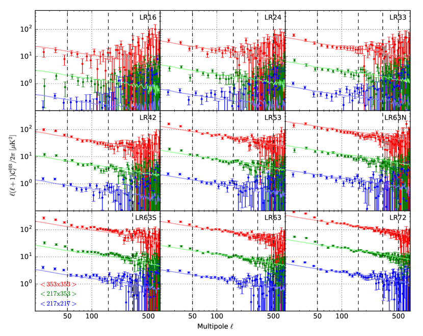
Figure 1: Half-mission cross spectra on the PIPL LR regions in bins of $\Delta\ell=10$. The points are the real data. Error bars are the standard deviation of the signal+noise simulations. Solid lines are the mean of the simulations. Vertical dashed lines indicate the bin edges used in PIPL. Bandpowers for $\ell=20-50$ are plotted for completeness but are not used in PIPL.

We construct 500 simulated sky maps for each data split at both 217 GHz and 353 GHz following the procedure outlined in PIPL. We generate noiseless, Gaussian realizations of galactic dust plus CMB using the synfast routine of the healpy wrapper to the HEALpix sky pixelization library (Górski et al., 2005). The input dust power spectra are power laws with spectral index $\alpha_{EE}=\alpha_{BB}=-2.42$ and amplitudes obeying the parameters listed in Table 1 of (Planck Collaboration et al., 2016c, hereafter PIPXXX). Each dust realization scales in frequency as a modified blackbody with $T_{d}=19.6$ K and $\beta_{d}=1.59$ (Planck Collaboration et al., 2014b, 2015). Because the LR16 region was defined specially for the analysis in PIPL and does not have corresponding parameters in PIPXXX, we linearly extrapolate the dust amplitude as a function of $f_{sky}$ to 0.2 to find $A^{EE}=25.0~{}\mu\mathrm{K}^{2}$. (Extrapolating as function of neutral hydrogen column density $N_{\textsc{HI}}$ yields $A^{EE}=28.0~{}\mu\mathrm{K}^{2}$.) We assume the same $BB/EE$ ratio as LR24, $A^{BB}/A^{EE}=0.49$.

The input CMB power spectra are generated with the CAMB software using the best fit $\Lambda\mathrm{CDM}$ model from Planck Collaboration et al. (2014c). (Using the more recent 2015 cosmological parameters from Planck makes negligible difference.) The lensing $B$-mode (Zaldarriaga and Seljak, 1998) is included by setting the input $BB$ power spectrum to its expected value and, as such, does not contain off-diagonal power. This is unimportant for the current study. As in PIPL, we produce independent dust and CMB realizations for each of the LR regions. The realization is held fixed between frequencies, with only the dust amplitude changing.

We construct alternative dust simulations using the PySM software, a simple Python implementation of the Planck Sky Model (PSM) (Delabrouille et al., 2013; Thorne et al., 2017). We run the software with dust models 1 and 2. Dust model 1 scales the dust template in frequency according to the $\beta_{d}$ and $T_{d}$ maps measured from unpolarized Planck data. Dust model 2 scales the dust template in frequency using a $\beta_{d}$ map that is drawn from a Gaussian of $\mu=1.59$ and which, after smoothing on degree scales, has $\sigma=0.2$. Both dust model 1 and dust model 2 are reported in Thorne et al. (2017) to be consistent with Planck data. Dust model 2 produces much more decorrelation than dust model 1 (see Figure 5). We note that there is only a single PySM dust realization, which remains fixed between realizations and LR regions in these simulations.

Also as in PIPL, we construct noise realizations as random Gaussian realizations of $Q$ and $U$ maps obeying the 4x4 $QU$ covariance matrix which Planck provides for every map pixel of every data split. By construction in these simulations, noise between pixels and between data splits is uncorrelated. We produce 500 full sky noise realizations and hold these fixed between LR regions so that, as in the data, there is a common component to the noise in each of the nested LR regions. This differs from PIPL, which reports that they produce independent noise realizations for each of the LR regions.

Additionally, we use the Full Focal Plane Monte Carlo noise simulations, namely the FFP8 simulations (Planck Collaboration et al., 2016d), as an alternative to the $QU$ covariance noise simulations for the HM split. PIPL reports that they did not use the FFP8 maps directly as input realizations because of the presence of instrumental noise in the polarized dust component of the PSM. The FFP8 Monte Carlo noise realizations contain only simulated noise, however, and are unaffected by this issue. PIPL also reports that the FFP8 noise realizations that are available through the Planck Legacy Archive (PLA) are in good agreement with the noise realizations constructed from the corresponding $QU$ covariance maps. Though we confirm this agreement, only the full mission, full detector set FFP8 noise simulations are available through the PLA. Because both this analysis and that in PIPL use cross spectra between data splits, the publicly available FFP8 noise simulations are not directly useful for the current analysis. We therefore requested and obtained 1000 realizations of the HM split FFP8 noise simulations at 217 GHz and 353 GHz and 100 realizations at other frequencies. These have subsequently been made publicly available via the Planck data archive hosted on NERSC.

Unlike the $QU$ covariance noise simulations, the FFP8 simulations are expected to reproduce any noise correlations between data splits produced by the Planck map making procedure. We therefore use the FFP8 noise realizations in Section III.1 to determine any noise bias present in the data splits. All other results presented in this paper use the $QU$ covariance noise realizations.

II.2 Map preparation

The publicly available PIPL mask is provided at a HEALpix resolution of Nside=512. The publicly available Planck HFI maps are provided at the higher resolution of Nside=2048. PIPL does not describe their procedure for either downgrading the resolution of the HFI maps or upgrading the resolution of the mask. We opt to downgrade the HFI map resolution by averaging the sets of Nside=2048 pixels that form an Nside=512 pixel. (We use the healpy ud_grade utility.) The full resolution FFP8 noise realizations contain a number of unseen entries in the HM split that are not present in the data maps. We therefore mask these pixels and exclude them from the average in every map at every frequency prior to downgrading. This has the effect of increasing the effective noise in those Nside=512 pixels that contained an unseen in the superset of Nside=2048 pixels that constitute it. We fully account for this by generating the noise realizations at the native resolution of Nside=2048 and applying the mask in the same manner as we apply it to the real data.

We generate realizations of noiseless $a_{lm}$’s for CMB and dust and add them together with the appropriate frequency scaling for 217 GHz and 353 GHz (see Section II.1). We then multiply the $a_{lm}$’s by the Gaussian beam window function appropriate for the HFI 217 and 353 GHz beams (4.99 and 4.82 arcmin FWHM, respectively). We also multiply the $a_{lm}$’s by the HEALpix pixel window function appropriate for an Nside=512 map to capture power suppression from binning into pixels. Any effects from not generating the maps at the full resolution and applying the unseen mask are restricted to the pixel scale ($\ell\sim 1500$) and are thus irrelevant for the subsequent analysis. We then add the signal realizations and downgraded noise realizations to produce the final simulated maps (referred to as signal + noise simulations).

II.3 Power spectrum estimation

As in PIPL, we use the XPol power spectrum estimator (Tristram et al., 2005) to derive our main results. We also obtain similar results with the PolSpice estimator (Chon et al., 2004). Both estimators correct for $EB$ mixing in the mean resulting from incomplete sky coverage. PolSpice does no binning in $\ell$ and returns $\mathcal{C}_{\ell}=\left<a_{\ell m}a_{\ell m}^{*}\right>$. XPol requires the user to specify multipole bins and returns $\mathcal{D}_{\ell}=\ell(\ell+1)\mathcal{C}_{\ell}/2\pi$. In broad bins, we obtain consistent results between the two estimators only when we multiply PolSpice $\mathcal{C}_{\ell}$s by $\ell(\ell+1)/2\pi$ (to make them $\mathcal{D}_{\ell}$s) prior to binning. In the main results derived in this work using the HM and DS splits, we specify bins of width $\Delta\ell=5$ to XPol and re-bin these spectra to produce broader bins. We find this gives consistent results compared to specifying the broad bins to XPol directly. Binned $\mathcal{D}_{\ell}$’s are referred to as “bandpowers.” In Section V, we compute the unbinned spectra of additional splits to assess the level of systematics in the data. For these results we use the PolSpice estimator.

We apply the estimator to the signal + noise simulations and to the real data. We also apply it to the signal and noise simulations separately. At each frequency, we compute the cross spectrum between the HM or DS split halves:

$$\mathcal{C}_{\ell}^{XX}(\nu\times\nu)=\mathcal{C}_{\ell}^{XX}(\mathrm{map}_{\nu}^{1}\times\mathrm{map}_{\nu}^{2})$$ (2)

where $XX\in{EE,BB}$ and the superscripts $1$ and $2$ denote the split half. As in PIPL, we also compute the cross spectrum between frequencies by taking the mean of all four independent crosses:

$$\mathcal{C}_{\ell}^{XX}(\nu_{1}\times\nu_{2})=\frac{1}{4}\sum_{i,j}\mathcal{C}_{\ell}^{XX}(\mathrm{map}_{\nu_{1}}^{i}\times\mathrm{map}_{\nu_{2}}^{j})$$ (3)

where $i$ and $j$ take the values 1 and 2, representing the two independent splits. As long as the noise is uncorrelated between all four $\mathrm{map}_{\nu}^{i}$, the cross spectra computed with Eqs. 2 and 3 have no additive noise bias.

III Power spectrum Results

Figure 1 shows the $BB$ intra- and inter-frequency cross spectra on each LR region computed from the HM split using Eqs. 2 and 3. The spectra are binned into bandpowers of width $\Delta\ell=10$. The agreement between the real data and the mean of simulations indicates the appropriateness of our simulations for modeling the real data. (Ultimately, this indicates the appropriateness of the dust power law parameters in Table 1 of PIPXXX for describing the galactic dust in these regions of sky.) We attribute the slight deviation of the real data from the simulations in the LR63S and LR63N regions to the fact that dust power law parameters are only available for the full LR63 region and would be somewhat different if fit for separately on the north and south patches.

The DS split power spectra (not shown) are consistent over all multipoles to within twice the total error bars shown in Figure 1, indicating the relative unimportance of instrumental systematics for measuring quantities affected by dust sample variance, such as the dust power law parameters. We do not have the DS split FFP8 noise simulations and therefore cannot assess the consistency of the HM and DS bandpowers to the level of instrumental noise. We therefore cannot test for HM-DS data consistency at the level required for super-sample variance measurements, such as the decorrelation parameter introduced in the next section.

III.1 Intra-frequency noise correlations

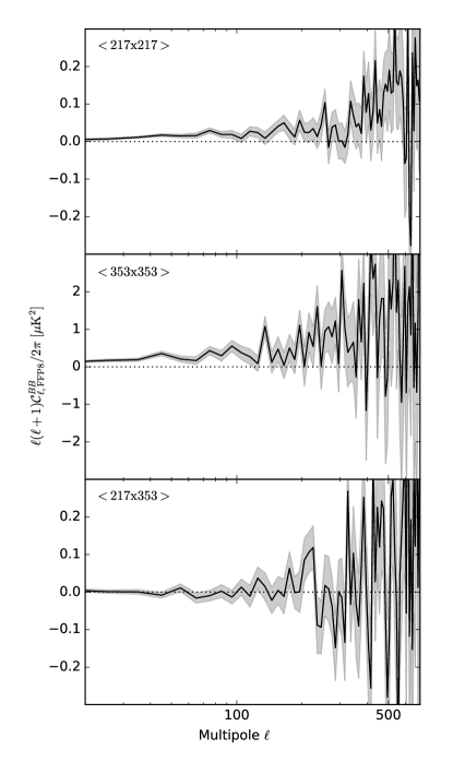
Figure 2: Half-mission cross spectra of the FFP8 Monte Carlo noise simulations in the LR63 region. The binning is the same as in Figure 1. The solid line is the mean over FFP8 realizations and the shaded region is the standard error, computed as the standard deviation over realizations divided by the square root of the the number of realizations.

With the FFP8 HM noise simulations we can test for noise bias in the power spectra shown in Figure 1. Figure 2 shows the HM cross spectra of the FFP8 HM noise simulations on the LR63 region. These spectra indicate significant positive bias in $217\times 217$ and $353\times 353$, and no bias in $217\times 353$. The bias ranges from $\sim 1\%$ of the dust signal at $\ell=50$ to $\sim 15\%$ at $\ell=700$ in $217\times 217$. The bias is similar in other LR regions but is measured with somewhat less statistical precision. There is no measured bias in the $QU$ covariance generated noise simulations.

Such a bias in the Planck data is expected given the destriping procedure described in Planck 2015 VIII, Section 6.5, which describes the trade-off in accuracy vs. noise correlation given the choice of using a baseline offset computed for each subset independently (lower accuracy but maintains independent noise), or using the full frequency, full mission baselines to destripe the subset halves (higher accuracy at the cost of introducing noise correlations). The Planck 2015 HFI data release uses the latter destriping procedure. The text of Planck 2015 VIII explicitly states that full mission destriping introduces noise correlations between detector set maps, and Figure 17 of that paper shows the FFP8 detector-set $EE$ noise cross spectrum at 100 GHz, which peaks at $\mathcal{C}_{\ell}\sim 0.0035~{}\mu\mathrm{K}^{2}$ at $\ell=2$ and falls steeply with $\ell$, though still appears visibly positive at $\ell=50$. (In Figure 2 of this work, the bias appears to increase with $\ell$ because of the $\ell^{2}$ scaling.) This amplitude matches the noise correlation we observe in the 100 GHz half-mission FFP8 noise cross spectrum (not shown). We have verified that the destriping procedure produces similar correlations in the half-mission split noise cross spectra, and that the FFP8 noise simulations include these induced noise correlations (private communication, J. Borrill). We therefore conclude that the noise correlation shown in Figure 2 is present in both the Planck 2015 HM and DS split maps. We note that PIPL does not account for any bias introduced by noise correlations.

Assuming that the signal is the same in each data subset and that it is uncorrelated with noise, the total measured cross spectrum is $\left<(S+N_{1})(S+N_{2})\right>=\left<S^{2}\right>+\left<N_{1}N_{2}\right>$ where $S$ is the signal and $N_{i}$ is the noise in each subset. Figure 2 shows the relatively small but important correlated noise term $\left<N_{1}N_{2}\right>$, which must be subtracted (i.e. “debiased”) from the measurement.

IV Decorrelation

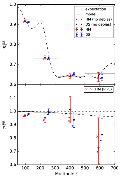
Figure 3: Correlation ratios $\mathcal{R}_{\ell}^{EE}$ (top panel) and $\mathcal{R}_{\ell}^{BB}$ (bottom panel) in the LR63 region. Correlation ratios calculated from the HM and DS splits are shown as the red diamonds and blue squares, respectively. The red and blue dots are the correlation ratios computed from the same spectra but without debiasing the expected noise correlation. The red x’s in the bottom panel are $\mathcal{R}_{\ell}^{BB}$ reported in the appendix of PIPL, which are directly comparable to the red dots. The dashed black line is the expected correlation ratio given the relative amplitudes of dust and CMB in the LR63 region. The model expectation values are shown as gray horizontal lines indicating the bin. The error bars are computed as the median absolute deviation of the signal+noise simulations.

IV.1 Correlation ratio

We compute the correlation ratio between 217 and 353 GHz, defined in PIPL as

$$\mathcal{R}_{\ell}^{XX}=\frac{\mathcal{C}_{\ell}^{XX}(353\times 217)}{\sqrt{\mathcal{C}_{\ell}^{XX}(353\times 353)\mathcal{C}_{\ell}^{XX}(217\times 217)}}$$ (4)

where $XX\in{EE,BB}$. Eq. 2 is used to compute the two terms in the denominator and Eq. 3 is used to compute the numerator. Any operation which multiplies the $a_{lm}$’s of a given map by an arbitrary function of $\ell$ cancels in the correlation ratio. Therefore $\mathcal{R}_{\ell}$ is unaffected by convolution with a circularly symmetric beam, multiplication by the pixel window function, or by many calibration errors. (In principle, the beam window functions for the detector-set cross do not perfectly cancel in the ratio. We have verified using the HFI beam window functions provded in the Planck Reduced Instrument Model that the non-cancellation produces deviations of $\mathcal{R}_{\ell}<10^{-6}$ at $\ell<700$.)

If there is no noise bias or instrumental systematics and the sky at 217 GHz is perfectly spatially correlated with the sky at 353 GHz, then $\mathcal{R}_{\ell}^{XX}=1$. Such would be the case if the maps contained a single component with a spatially invariant spectral energy distributions (SED). If two or more components with different SEDs contribute to the maps then they deviate from perfect spatial correlation and $\mathcal{R}_{\ell}<1$. We expect this decorrelation from the admixture of dust and CMB. In $BB$, only the lensing $BB$ produces this decorrelation. Since the lensing $BB$ is small compared to the dust at low $\ell$, the amount of decorrelation it produces is quite small and relatively immune to assumptions about the relative power in the two components.

Lastly, additional decorrelation will be produced if any component contains a spatially varying SED, for instance, from a spatially dependent $\beta_{d}$ or from polarization angle rotations. As noted in the introduction, such effects are predicted to exist at a small level (Tassis and Pavlidou, 2015; Poh and Dodelson, 2017).

Figure 3 is analagous to Figure 2 of PIPL and shows $\mathcal{R}_{\ell}^{EE}$ and $\mathcal{R}_{\ell}^{BB}$ for the LR63 region using the same four bins as PIPL ($\ell=50-160$, $\ell=160-320$, $\ell=320-500$, and $\ell=500-700$). As in PIPL, the error bars are computed as the median of the absolute deviation of the signal + noise simulations. Prior to noise debiasing, we find nearly exact agreement with PIPL in $\mathcal{R}_{\ell}^{BB}$ in the first two bins for the HM split. In the last two bins there are small, $<1\sigma$ shifts in $\mathcal{R}_{\ell}^{BB}$. (As stated in Section II, the DS split is not exactly comparable with PIPL.) Noise debiasing results in a $\sim 1\sigma$ shift upwards in $\mathcal{R}_{\ell}^{BB}$ in the first bin for both the the HM and DS splits.

In $\mathcal{R}_{\ell}^{EE}$ there are two significant differences with the figure in PIPL. First, we find significantly smaller error bars for $\mathcal{R}_{\ell}^{EE}$ compared to $\mathcal{R}_{\ell}^{BB}$. This is perhaps because PIPL appears to transfer the $\mathcal{R}_{\ell}^{BB}$ error bars onto the $\mathcal{R}_{\ell}^{EE}$ bandpowers. Second, our model expectation values differ somewhat from PIPL due to more careful binning. We can reproduce the PIPL results by binning the $\mathcal{R}_{\ell}$ model curve computed from unbinned model spectra. Where $\mathcal{R}_{\ell}$ is changing rapidly, this can produce significant shifts in the expectation values compared to binning the constituent spectra, which is the procedure that is consistent with how the data are treated.

Because the $\Lambda\mathrm{CDM}$ $E$-mode power is similar in amplitude to dust power, we find that the expected $EE$ decorrelation is significantly affected by the assumed amplitude of dust power in each $\ell$ bin. Noiseless simulations run with PySM modified to produce zero decorrelation show significant deviations from the $EE$ model curve in Figure 3. Because dust is the only significant contributor to the $B$-mode power, however, there is almost no dependence of $\mathcal{R}_{\ell}^{BB}$ on $\Lambda\mathrm{CDM}$ sample variance or the assumed dust amplitude. Accordingly, the PySM simulations show excellent agreement with the $BB$ model curve in Figure 3. Therefore, as in PIPL, we only use $\mathcal{R}_{\ell}^{BB}$ to derive results.

IV.2 Alternative binning

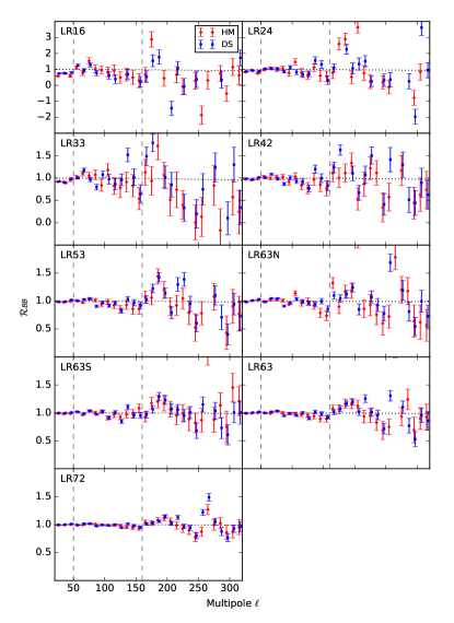
Figure 4: Noise debiased $\mathcal{R}_{\ell}^{BB}$ on all LR regions in bins of width $\Delta\ell=10$. The HM and DS splits are shown as red and blue points, respectively. The error bars are computed as the standard deviation of the signal+noise simulations. The dashed vertical gray lines indicate the PIPL bin edges. The dotted line is the model expectation value.

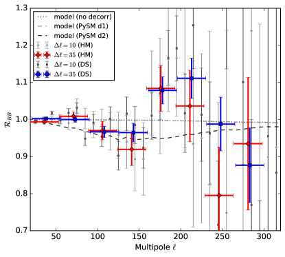
Figure 5: Noise debiased $\mathcal{R}_{\ell}^{BB}$ on the LR63 region. The gray points are the same HM and DS data points shown in Figure 4. The red diamonds and blue squares use an alternative binning of $\Delta\ell=35$ beginning from $\ell=20$. Error bars are the standard deviation of the signal+noise sims. The dotted black line shows the $\mathcal{R}_{\ell}^{BB}$ model expectation for no dust decorrelation. The dashed gray/black lines show the decorrelation produced by PySM dust model 1/2. PySM dust model 1 is indistinguishable from the no decorrelation model.

We now compute $\mathcal{R}_{\ell}^{BB}$ using finer bins than presented in PIPL. Figure 4 shows $\mathcal{R}_{\ell}^{BB}$ computed from binning $\mathcal{D}_{\ell}$ in bins of $\Delta\ell=10$ (i.e. the same spectra shown in Figure 1). Figure 5 shows the LR63 panel, adding bins of $\Delta\ell=35$ starting from $\ell=20$. We choose these latter bins to be the same as the bins used in the BICEP-Planck joint analysis. The $\ell=55-90$ bin has comparable signal-to-noise as the $\ell=50-160$ bin and shows no evidence for decorrelation in either the HM or DS splits. It appears inconsistent with the flat decorrelation assumed by PIPL ($\mathcal{R}_{50-160}^{BB}=0.95$). It also appears inconsistent with PySM dust model 2. It is consistent with both the no-decorrelation model and PySM dust model 1, which shows negligible additional decorrelation from the no-decorrelation model.

V Systematics

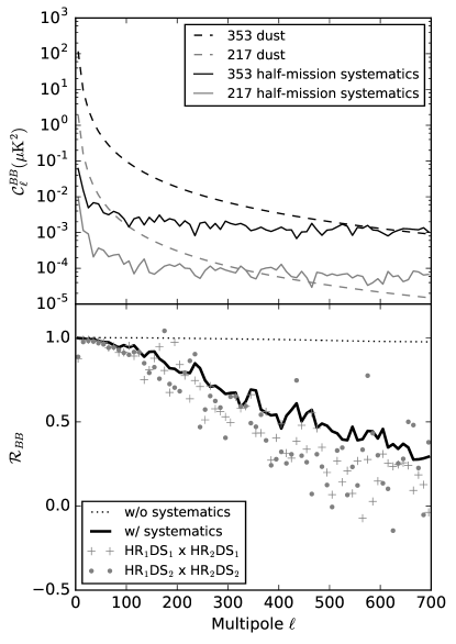
Figure 6: Top panel: Model dust $\mathcal{C}_{\ell}^{BB}$ for 353 GHz and 217 GHz (dashed lines) in LR72, and excess power in the HM map difference null test relative to the FFP8 noise simulations (solid lines). Bottom panel: Predicted $\mathcal{R}_{\ell}^{BB}$ in LR72 with no decorrelation and no systematics (dotted black line) and in the presence of systematics given by the solid lines in the top panel (solid black line). The data points are the measured $\mathcal{R}_{\ell}^{BB}$ computed from the half-ring split for each detector set separately.

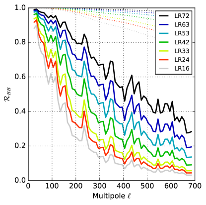
Figure 7: Expectation for $\mathcal{R}_{\ell}^{BB}$ in the presence of a correlated systematic of the same amplitude as the uncorrelated systematic shown in Figure 6. The expectation without systematics is given by the corresponding dotted lines.

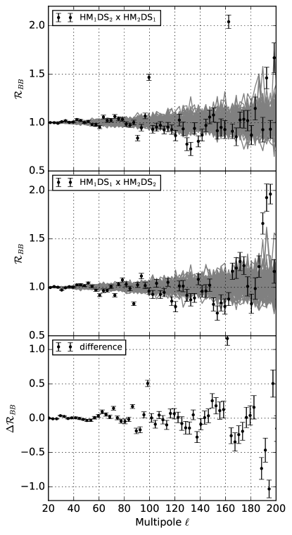
Figure 8: Top and middle panels: $\mathcal{R}_{\ell}^{BB}$ on LR72 measured in bins of $\Delta\ell=3$ using two independent cross spectra of the four HM_iDS_j data splits. The black points are the data. The error bars are computed as the standard deviation of 100 corresponding signal+noise simulations with the signal realization held fixed, which are shown as gray lines. Points with error bars should be compared to $1$ rather than to the simulations, which are shown only to give a visual indication of the distribution. Bottom panel: the difference, $\Delta\mathcal{R}_{\ell}^{BB}$, between the data points in the top and middle panels, which should be consistent with zero. The error bars are the standard deviation of the corresponding differences between simulation realizations.

The use of cross spectra to calculate the denominator of Eq. 4 means that $\mathcal{R}_{\ell}$ will be biased by the presence of systematics that correlate between either halves of the HM or DS split or between 217 and 353. Figure 11 of Planck 2015 VIII shows a clear failure of map difference null tests constructed from single-frequency data splits, $\mathrm{map}^{\mathrm{HM}_{1}}_{\nu}-\mathrm{map}^{\mathrm{HM}_{2}}_{\nu}$ and $\mathrm{map}^{\mathrm{DS}_{1}}_{\nu}-\mathrm{map}^{\mathrm{DS}_{2}}_{\nu}$. There is significant excess power in the difference maps compared to power in difference maps of the corresponding FFP8 noise simulations. Planck 2015 VIII attributes this to instrumental systematics, and a subsequent paper (Planck Collaboration et al., 2016e) finds it to be largely the result of non-linearity in the analog-to-digital converter.

Instrumental systematics that contaminate a map difference null test are by definition uncorrelated between data halves. As such, they do not bias $\mathcal{R}_{\ell}$. We can predict what bias such a systematic would produce were it instead correlated between data splits. The top panel of Figure 6 shows the LR72 model dust spectra at 217 and 353 compared to the uncorrelated systematics in the HM maps, which we compute as the excess power in the HM difference maps compared to the FFP8 noise simulations:

$$\mathcal{C}_{\ell}^{syst} = \mathcal{C}_{\ell}[(\mathrm{map}_{\nu}^{\mathrm{HM_{1}^{data}}}-\mathrm{map}_{\nu}^{\mathrm{HM_{2}^{data}}})/2]-$$

$$\left<\mathcal{C}_{\ell}[(\mathrm{map}_{\nu}^{\mathrm{HM_{1}^{FFP8}}}-\mathrm{map}_{\nu}^{\mathrm{HM_{2}^{FFP8}}})/2]\right>.$$

where the expectation value is taken over realizations.

The 217 systematics curve in Figure 6 is comparable to the difference between the “Half Mission” and “FFP8” lines in the bottom panel of Fig. 11 of Planck 2015 VIII. (The main difference is that the present work shows $BB$ systematics while the Planck figure shows $EE$ systematics.) Both figures show excess power in 217 of $\sim 10^{-2}~{}\mu\mathrm{K}^{2}$ at $\ell=10$ and $\sim 10^{-4}~{}\mu\mathrm{K}^{2}$ at $\ell=100$. We therefore conclude that the uncorrelated systematics in the 217 HM split maps dominate the LR72 dust signal at $\ell>300$ and are $10\%$ of the dust signal at $\ell=50$. In the 353 maps, the systematics are fractionally lower relative to the dust signal but are still $10\%$ at $\ell=150$.

The black line in the bottom panel of Figure 6 shows the expected bias on $\mathcal{R}_{\ell}$ that such a systematic would produce in LR72 if it were instead correlated between data split halves. One such data split that preserves correlations of instrumental systematics is the HR split. The data points in the bottom panel of Figure 6 show $\mathcal{R}_{\ell}^{BB}$ computed from HR cross spectra of maps built from individual detector sets. There is a large downward bias on $\mathcal{R}_{\ell}^{BB}$ whose magnitude is comparable to the level predicted from the HM map difference null test. The fact that a bias of this magnitude is not observed in $\mathcal{R}_{\ell}$ computed from HM or DS cross spectra indicates that the portion of instrumental systematics that is correlated between the data split halves is small compared to the uncorrelated portion. However, if even a small fraction of this systematic were correlated, it would produce a bias on $\mathcal{R}_{\ell}^{BB}$ that is significant compared to the measurement uncertainty.

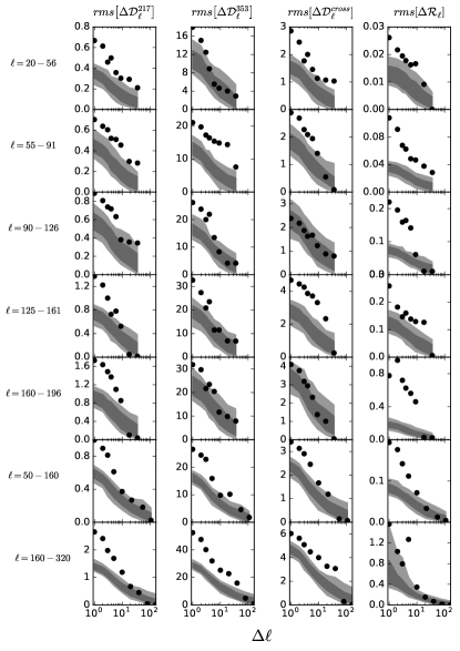
Figure 9: Root-mean-square (rms) of the difference $\Delta\mathcal{D}_{\ell}^{BB}$ and $\Delta\mathcal{R}_{\ell}^{BB}$ between the two independent cross spectra of the four HM_iDS_j data splits. The left three columns show $\Delta\mathcal{D}_{\ell}^{BB}$ in $\mu\mathrm{K}^{2}$ for $217\times 217$, $353\times 353$, and $217\times 353$. The right column shows $\Delta\mathcal{R}_{\ell}^{BB}$. Each row shows the rms computed in the indicated broad multipole bin. The $x$-axis of each panel indicates the fine binning of the raw spectra from which the rms values are calculated in the broad bins. The binning ranges from $\Delta\ell=1$ to the full bin width. The dark and light gray regions enclose $68\%$ and $95\%$ of the corresponding signal+noise simulations.

Figure 7 shows the bias on $\mathcal{R}_{\ell}^{BB}$ in each LR region from a correlated systematic of the magnitude of the uncorrelated systematic measured in the LR72 region. We note again that the excess power in the HM map difference null test does not appear to change in amplitude in smaller sky fractions.

To assess the level of correlated systematics in the HM and DS splits, which will not contaminate the map difference null tests, we perform a difference-of-bandpowers null test on $\mathcal{D}_{\ell}^{BB}$ and $\mathcal{R}_{\ell}^{BB}$ computed from the HM_iDS_j splits. Each of these four splits contains 1/4th of the total nominal mission data and is independent of the others. (For example, HM₁DS₂ is the quarter of the data that belongs to half-mission one and detector-set two.) We compute bandpowers and $\mathcal{R}_{\ell}^{BB}$ from what should be the two maximally uncontaminated cross spectra: HM₁DS₂ $\times$ HM₂DS₁ and HM₁DS₁ $\times$ HM₂DS₂. We then take the difference of bandpowers, $\Delta\mathcal{D}_{\ell}^{BB}$, and the difference of the correlation ratios, $\Delta\mathcal{R}_{\ell}^{BB}$ and compare them to the corresponding differences calculated from signal+noise simulations. The simulations are constructed from a fixed signal realization and 100 noise realizations constructed from the four $QU$ covariance maps of the HM_iDS_j splits.

The top and middle panels of Figure 8 show the two independently measured $\mathcal{R}_{\ell}^{BB}$ in bins of $\Delta\ell=3$ along with the 100 signal+noise simulations for reference. The bottom panel shows the difference, $\Delta\mathcal{R}_{\ell}^{BB}$ . (The simulation realizations are omitted in the bottom panel for clarity but, similarly to the top and middle panels, they show no outlying realizations.) Deviation of $\Delta\mathcal{R}_{\ell}^{BB}$ from zero in the bottom panel is evidence for correlated systematic contamination between the HM and DS split halves. The outlier points in the top and bottom panel are real. However, only 100 simulation realizations are plotted, and because of the high side tail of the likelihood distribution ($\mathcal{R}_{\ell}^{BB}$ is a ratio whose denominator can be close to zero due to noise fluctuations) the likelihood of these fluctuations is probably underestimated by the size of the error bars. The known uncorrelated systematics act to increase the effective noise in this null test, which we do not account for. Nevertheless, the excess uncorrelated power is $\lesssim 20\%$ of the total noise power and thus cannot explain the observed discrepancies.

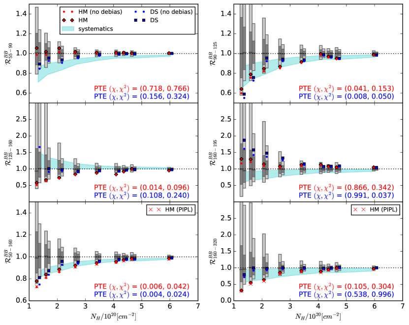
Figure 10: $\mathcal{R}_{\ell}^{BB}$ in the 9 LR regions, plotted as a function of neutral hydrogen column density, $N_{\textsc{HI}}$. Each panel is a different multipole bin. The red diamonds and and blue squares show $\mathcal{R}_{\ell}^{BB}$ calculated from the HM and DS splits, respectively. The corresponding red and blue dots show $\mathcal{R}_{\ell}^{BB}$ without accounting for noise bias. The vertical bars indicate the regions enclosing $68\%$ and $95\%$ of the signal+noise simulations ($16-84$ and $2.5-97.5$ percentiles, respectively) and the dark gray horizontal lines show the median of the simulations. The red x’s in the bottom two panels show the corresponding PIPL points, taken from the appendix, which should be the same as the “HM (no debias)” points. In each panel there are four statistics listed: the $\chi$ and $\chi^{2}$ PTE for the HM and DS splits, calculated as the number of simulations having $\chi$ ($\chi^{2}$) less (greater) than the observed value. A low/high $\chi$ PTE indicates data that is coherently low/high. A low/high $\chi^{2}$ PTE indicates data that has too much/little scatter. The PTEs do not account for systematic uncertainty. The cyan shaded region indicates the region between the pessimistic and optimistic estimates of the systematic bias on $\mathcal{R}_{\ell}^{BB}$, computed as the expectation for $\mathcal{R}_{\ell}^{BB}$ in the presence of a systematic upward bias on $\mathcal{D}_{\ell}^{BB}$ given by Eq. 6 and the $\Delta\ell=3$ (pessimistic) and $\Delta\ell=$ full width/2 (optimistic) data in Figure 9.

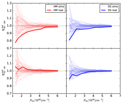
Figure 11: $\mathcal{R}_{\ell}^{BB}$ in the 9 LR regions plotted as a function of neutral hydrogen column density, $N_{\textsc{HI}}$. The left and right columns are the HM and DS splits, respectively. The top and bottom rows are the $\ell=50-160$ bin and $\ell=55-90$ bin, respectively. The thick line shows the real data and is the same as the noise debiased points in the corresponding panels of Figure 10. The thin lines show the first 50 signal+noise realizations. The only component held fixed between LR regions in a single simulation realization is the $QU$ covariance generated noise map.

Figure 9 shows the root-mean-square (rms) of $\Delta\mathcal{R}_{\ell}^{BB}$ and $\Delta\mathcal{D}_{\ell}^{BB}$ (not shown) calculated in 7 different $\ell$ bins. Also plotted are the regions enclosing $68\%$ and $95\%$ of the rms values from simulation. The rms is calculated in each $\ell$ bin from more finely binned data with fine bin width $\Delta\ell$ ranging from 1 to the full bin width, purposefully chosen in some bins to be $\Delta\ell=36$, which has many divisors, instead of $\Delta\ell=35$, which does not. (For instance, Figure 8 shows $\Delta\mathcal{R}_{\ell}^{BB}$ in bins of $\Delta\ell=3$, and the corresponding $rms[\mathcal{R}_{\ell}^{BB}]$ is plotted as the $\Delta\ell=3$ points in the right hand column of Figure 9.) When $\Delta\ell$ is equal to the full bin width, the rms is simply the absolute value of the difference of two points.

We find strong disagreement between the observed and simulated rms values in finely binned spectra. For the full bin width, we find general agreement, except for in the $\ell=20-56$ and $\ell=55-91$ bin. The behavior of the observed rms indicates a systematic that at least partially averages down when binning in $\ell$. We can see this in Figure 8: apparent correlated structure in $\Delta\mathcal{R}_{\ell}^{BB}$ will average to zero in broad $\ell$ bins, resulting in agreement with simulations. It is unknown whether the total correlated systematics will also average down – the bandpower difference null test uncovers systematics that are correlated within each of the two pairs of HM_iDS_j and yet produce a different bias in the two cross spectra. Systematics that produce the same bias in each cross spectrum will not produce null test failures.

We therefore adopt $\Delta\ell=\mathrm{full~{}width}/2$ as an optimistic estimate of the systematic contamination due to instrumental systematics and $\Delta\ell=3$ as a pessimistic case. We then compute the expected bias on $\mathcal{D}_{\ell}$ as one half the observed minus the mean simulated rms:

$$\mathcal{D}_{\ell}^{s,syst}=\frac{1}{2}\left(rms\left[\Delta\mathcal{D}_{\ell}^{s,obs}\right]-\left<rms\left[\Delta\mathcal{D}_{\ell}^{s,sim}\right]\right>\right)$$ (6)

where $<>$ is the mean over simulations; $s=217$, $353$, or $cross=217\times 353$; and the factor $1/2$ assumes that the magnitude of the null test failure is twice the contamination in each cross spectrum individually. We set $\mathcal{D}_{\ell}^{syst}=0$ if it is $<0$. We then use these estimates of the bias in the next section to estimate the bias on $\mathcal{R}_{\ell}^{BB}$ in each LR region.

VI Significance of measurements

VI.1 Trends with sky fraction

Figure 10 shows $\mathcal{R}_{\ell}^{BB}$ in 6 separate $\ell$ bins, plotted as a function of the mean neutral hydrogen column density, $N_{\textsc{HI}}$, in each LR region as reported in PIPL. The HM data in the bottom two panels are directly comparable to $\mathcal{R}_{\ell}^{BB}$ reported in PIPL, and we find very good agreement. (We note that this agreement is true of the $\mathcal{R}_{\ell}^{BB}$ values shown in the histograms plotted in the appendix of PIPL. The $\mathcal{R}^{BB}_{50-160}$ points plotted in Figure 3 of PIPL appear inconsistent with both the current results and the appendix of PIPL.) The HM and DS splits are both plotted. Vertical bars indicate the regions enclosing $68\%$ and $95\%$ of the signal+noise simulations. Lastly, we plot the region between the “optimistic” and “pessimistic” systematic bias predictions discussed in the previous section and defined in Eq. 6.

To gauge the significance of any trends in Figure 10, we compute two statistics from both the real data and each simulation realization: the inverse variance weighted $\chi$ and $\chi^{2}$, defined as

$$\chi^{n}=\sum_{\mathrm{LR}}\left[(\mathcal{R}_{\ell}^{BB}-1)/\sigma_{\mathcal{R}_{\ell}^{BB}}\right]^{n}.$$ (7)

where $\sigma_{\mathcal{R}_{\ell}^{BB}}$ is the width of the $68\%$ confidence intervals shown in Figure 10. We then compute the probability to exceed (PTE) of these statistics. The $\chi$ PTE is defined as the fraction of simulations having $\chi$ less than the observed value, so that low/high PTEs indicate $\mathcal{R}_{\ell}^{BB}$ which is coherently low/high across LR regions. The $\chi^{2}$ PTE is defined as the fraction of simulations having $\chi^{2}$ greater than the observed value, so that a low PTE indicates data with too much scatter under the no decorrelation hypothesis.

Without accounting for instrumental systematics, the strongest disagreement with simulations comes from the $\ell=50-160$ DS split, with PTE${}_{\chi}=0.4\%$. The HM and DS split appear qualitatively consistent in this bin. Examining the $\ell=50-160$ sub-bins, however, we find, different results. Neither the $\ell=55-90$ bin, which has similar signal-to-noise to the full $\ell=50-160$ bin, nor the $\ell=125-160$ bin show strong evidence for decorrelation. In these two bins, apparent trends in either the DS or HM splits are not seen in the other split. The $\ell=90-125$ bin shows the largest downward deviation of $\mathcal{R}_{\ell}^{BB}$ from $1$ and has qualitative consistency between HM and DS.

The marginally low $\mathcal{R}_{\ell}^{BB}$ in the $\ell=50-160$ and $\ell=90-125$ bins are, however, fully consistent with the estimate of bias from instrumental systematics. Furthermore, the $\ell=160-195$ bin has DS PTE${}_{\chi}=0.991$, which is marginal evidence for the unphysical $\mathcal{R}_{\ell}^{BB}>1$. There is also an apparent trend to higher $\mathcal{R}_{\ell}^{BB}$ with lower $N_{\textsc{HI}}$ in this bin. This upward bias is possible if systematics correlate between 217 and 353, a possibility Figure 9 shows some evidence for. The “optimistic” systematics line in the $\ell=125-160$ panel of Figure 10 shows a positive bias because the corresponding $\Delta\ell=18$ $rms[\mathcal{D}_{\ell}]$ values in Figure 9 show no disagreement with simulations in $217\times 217$ or $353\times 353$ but a significant positive bias in $217\times 353$. This bin does show an upward fluctuation of $\mathcal{R}_{\ell}^{BB}$ in LR16 prior to noise debiasing. (After noise debiasing, $217\times 217$ becomes negative and $\mathcal{R}_{\ell}^{BB}$ becomes undefined.) We note, however, that in the $\ell=160-195$ bin, Figure 9 shows no evidence for problems with the $217\times 353$ cross spectrum.

Figure 11 shows the $\mathcal{R}_{50-160}^{BB}$ and $\mathcal{R}_{55-90}^{BB}$ data from Figure 10 plotted as thick lines and the first 50 realizations of the signal+noise simulations plotted as thin lines. Clear trends are visible in the simulations indicating significant correlation between LR regions. The PTEs listed in Figure 10 would be much more significant were it not for these correlations. The simulations are the $QU$ covariance noise realizations plus a Gaussian dust + CMB signal realization. Only the noise realization is common between the LR regions in a given realization. As in PIPL, the dust and CMB realizations change. We therefore conclude that the noise common to the nested LR regions is responsible for the correlations. This result is perhaps unsurprising given that $\mathcal{R}_{\ell}^{BB}$ is measured largely without sample variance. In simulations substituting the fixed PySM dust + CMB realization for the varying Gaussian dust + CMB realizations, we observe nearly identical correlations between LR regions. We also observe nearly identical correlations when we substitute in the FFP8 noise simulations for the $QU$ covariance noise realizations.

To see the correlations more clearly, Figure 12 shows the correlation coefficient matrix for $\mathcal{R}_{\ell}^{BB}$ between multipole bins and LR regions. In each bin, there are large correlations between LR regions except for 63N and 63S, which are non-overlapping. These correlations ensure that strong trends in $\mathcal{R}_{\ell}^{BB}$ as a function of $N_{\textsc{HI}}$ are expected even with no decorrelation. Measurements of $\mathcal{R}_{\ell}^{BB}$ in different LR regions may therefore not be regarded as approximately statistically independent, as advocated in PIPL. We do note that non-overlapping $\ell$ bins appear to be negligibly correlated, as expected.

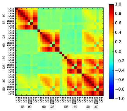
Figure 12: $\mathcal{R}_{\ell}^{BB}$ correlation coefficient between multipole bins and LR regions.

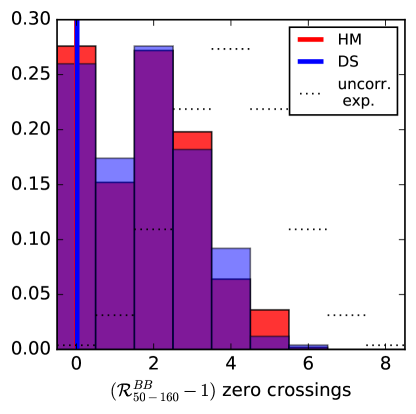
Figure 13: Number of zero crossings of $[\mathcal{R}^{BB}_{50-160}(N_{\textsc{HI}})-1]$ calculated from HM and DS splits (red and blue) and shown in the top left panel of Figure 10. The vertical lines are the observed values and the histograms are the distribution from the signal+noise simulations. The dotted histogram is the expectation for 9 uncorrelated random numbers distributed about 1 computed from the binomial distribution.

We also compute the number of zero crossings of $\mathcal{R}_{\ell}^{BB}(N_{\textsc{HI}})-1$ in the $\ell=50-160$ bin, which we show in Figure 13. The HM and DS data both have no zero crossings. If measurements of $\mathcal{R}_{\ell}^{BB}$ in different LR regions were uncorrelated, these results would be highly unlikely without significant dust decorrelation. This is evident from the dotted line histogram, which is the number of zero crossings predicted by the binomial distribution under the hypothesis that $\mathcal{R}_{\ell}>1$ and $\mathcal{R}_{\ell}<1$ are equally likely. We find, however, that in the simulations, which account for correlations between LR regions, observing no zero crossings is in fact one of the most likely outcomes.

VI.2 Maximum Likelihood $\mathcal{R}_{\ell}^{BB}$

Table 1 lists the maximum likelihood (ML) values of the noise debiased $\mathcal{R}_{\ell}^{BB}$ in each LR region and in different $\ell$ bins. (We also list the $\ell=50-160$ non-noise-debiased values for comparison.) We quote statistical uncertainties as empirically determined from the simulations. We adjust the simulations by adding or subtracting a constant value to each realization’s $217\times 353$ binned $\mathcal{D}_{\ell}$’s such that the mean decorrelation of the signal-only simulations equals the observed value. We leave the $217\times 217$ and $353\times 353$ $\mathcal{D}_{\ell}$’s alone under the assumption that small levels of decorrelation suppress power in the cross spectrum without significantly affecting the auto spectra. We then recompute $\mathcal{R}_{\ell}^{BB}$ of each realization and adopt this as the ML distribution. The statistical uncertainties, $\sigma_{\mathcal{R}_{\ell}^{BB}}$, quoted in Table 1 are defined such that $\mathcal{R}_{\ell}^{BB}\pm 2\sigma_{\mathcal{R}_{\ell}^{BB}}$ encloses $95\%$ of the adjusted simulations ($2.5-97.5$ percentiles). We also include data for the $\ell=20-55$ bin in LR72 and LR63. The dust amplitude is strong enough in these region that the known low-$\ell$ Planck systematics appear to produce only a small bias on $\mathcal{R}_{\ell}$. The systematic uncertainty quoted is the mean of the systematics region shown in Figure 10.

Because of the significant systematic uncertainty in every bin and every LR region, we advocate that the ML values listed in Table 1 only be interpreted in light of the systematic uncertainty. The absence of evidence for decorrelation in the $\ell=55-90$ bin therefore places strong constraints on the maximum possible level of decorrelation at the peak of the expected inflationary $B$-mode signal. For instance, taken at face value, dust model 2 of PySM is consistent with $\mathcal{R}_{90-125}^{BB}$ and $\mathcal{R}_{125-160}^{BB}$ measured in LR63 (see Figure 5), but the model appears strongly ruled out by $\mathcal{R}_{55-90}^{BB}$. Also apparently inconsistent is the flat decorrelation of $\mathcal{R}^{BB}_{50-160}=0.95$ assumed by PIPL to predict an expected bias on $r$.

Table 2 lists the corresponding $\mathcal{R}_{\ell}^{BB}$ PTE values, defined as the fraction of simulations having $\mathcal{R}_{\ell}^{BB}$ less than the observed value. The PTEs do not account for systematic uncertainty.

VII Conclusions

In this paper we have revisited the the evidence for decorrelation in the polarized dust signal in Planck data. We have made several improvements in our analysis over the Planck analysis. Our conclusions can be summarized as follows:

• The destriping procedure correlates noise between data splits, a small but statistically relevant bias that cross-correlation power spectrum estimation must correct for to avoid artificially lowering $\mathcal{R}_{\ell}$ measurements.

• The data split difference maps contain excess power that is not present in the FFP8 simulations, thus indicating the presence of uncorrelated systematics. We find that if contamination were present at this level in the cross spectra it would push $\mathcal{R}_{\ell}$ measurements far below the observed values. By using quarter data splits, we have estimated the order of magnitude of correlated systematics, which will bias $\mathcal{R}_{\ell}$. Since we find evidence for these systematics and cannot exclude that they will average down to negligible levels in broad bins, we conclude that $\mathcal{R}_{\ell}$ measurements should only be interpreted in light of the systematic uncertainties shown in Figure 10 and quoted in Table 1.

• Even taking the $\mathcal{R}_{\ell}$ measurements at face value, at a fixed angular scale, the results from nested sky cuts are heavily correlated. Once these correlations are taken into account, the evidence for deviation from unity weakens significantly.

We have employed two statistics to quantify the discrepancy from the null hypothesis $\mathcal{R}_{\ell}^{BB}=1$ everywhere. The $\chi^{2}$ statistic calculates the average discrepancy with unity correlation while the $\chi$ statistic measures coherent shifts upwards or downwards. Although both statistics are generated using diagonal errors (of very strongly correlated covariance matrix), they are compared to simulations so that PTE values are valid (in the absence of systematics). Statistical evidence in the absence of systematics is weak, $2-3$ sigma. However, since we demonstrate the presence of an unknown systematic that can affect results at the level of the measurement accuracy, we must conservatively conclude that there is no statistically compelling evidence for decorrelation in the Planck data. Additional multifrequency data will be required to place stronger constraints on decorrelation.

Table 1: Noise debiased $\mathcal{R}_{\ell}^{BB}$ in different multipole bins and different LR regions measured with the HM and DS splits. The undebiased $\ell=50-160$ bin is also listed for comparison to the noise debiased values. The quoted statistical uncertainties are one half of the region enclosing $95\%$ of the adjusted signal+noise simulations. The systematic uncertainties are the mean of the optimistic and pessimistic systematics estimates shown in Figure 10.

	LR16	LR24	LR33	LR42	LR53	LR63N	LR63	LR63S	LR72
$f_{\rm sky}^{\rm eff}$ [%]	16	24	33	42	53	33	63	30	72
$\ell$ range	Maximum Likelihood $\mathcal{R}_{\ell}^{BB}(ML\begin{subarray}{c}+stat./syst.\\ -stat./syst.\end{subarray})$ ( HM DS )
50–160 (no d.b.)	$0.725\begin{subarray}{c}+0.20/0.16\\ -0.10/0.00\end{subarray}$ $0.748\begin{subarray}{c}+0.12/0.16\\ -0.08/0.00\end{subarray}$	$0.808\begin{subarray}{c}+0.10/0.12\\ -0.07/0.00\end{subarray}$ $0.837\begin{subarray}{c}+.064/.124\\ -.048/.000\end{subarray}$	$0.860\begin{subarray}{c}+.075/.100\\ -.053/.000\end{subarray}$ $0.929\begin{subarray}{c}+.043/.100\\ -.036/.000\end{subarray}$	$0.905\begin{subarray}{c}+.038/.065\\ -.033/.000\end{subarray}$ $0.937\begin{subarray}{c}+.023/.065\\ -.020/.000\end{subarray}$	$0.933\begin{subarray}{c}+.024/.043\\ -.021/.000\end{subarray}$ $0.952\begin{subarray}{c}+.014/.043\\ -.013/.000\end{subarray}$	$0.945\begin{subarray}{c}+.022/.028\\ -.018/.000\end{subarray}$ $0.968\begin{subarray}{c}+.012/.028\\ -.012/.000\end{subarray}$	$0.963\begin{subarray}{c}+.015/.028\\ -.012/.000\end{subarray}$ $0.972\begin{subarray}{c}+.008/.028\\ -.008/.000\end{subarray}$	$0.980\begin{subarray}{c}+.020/.028\\ -.016/.000\end{subarray}$ $0.974\begin{subarray}{c}+.011/.028\\ -.010/.000\end{subarray}$	$0.980\begin{subarray}{c}+.008/.018\\ -.007/.000\end{subarray}$ $0.985\begin{subarray}{c}+.004/.018\\ -.004/.000\end{subarray}$
50–160	$0.779\begin{subarray}{c}+0.21/0.16\\ -0.10/0.00\end{subarray}$ $0.811\begin{subarray}{c}+0.13/0.16\\ -0.08/0.00\end{subarray}$	$0.840\begin{subarray}{c}+0.11/0.12\\ -0.07/0.00\end{subarray}$ $0.872\begin{subarray}{c}+.066/.124\\ -.049/.000\end{subarray}$	$0.886\begin{subarray}{c}+.077/.100\\ -.054/.000\end{subarray}$ $0.958\begin{subarray}{c}+.044/.100\\ -.037/.000\end{subarray}$	$0.921\begin{subarray}{c}+.039/.065\\ -.033/.000\end{subarray}$ $0.954\begin{subarray}{c}+.024/.065\\ -.021/.000\end{subarray}$	$0.943\begin{subarray}{c}+.024/.043\\ -.021/.000\end{subarray}$ $0.962\begin{subarray}{c}+.014/.043\\ -.013/.000\end{subarray}$	$0.955\begin{subarray}{c}+.022/.028\\ -.018/.000\end{subarray}$ $0.978\begin{subarray}{c}+.012/.028\\ -.012/.000\end{subarray}$	$0.971\begin{subarray}{c}+.015/.028\\ -.012/.000\end{subarray}$ $0.980\begin{subarray}{c}+.008/.028\\ -.008/.000\end{subarray}$	$0.986\begin{subarray}{c}+.020/.028\\ -.016/.000\end{subarray}$ $0.980\begin{subarray}{c}+.011/.028\\ -.010/.000\end{subarray}$	$0.985\begin{subarray}{c}+.008/.018\\ -.007/.000\end{subarray}$ $0.990\begin{subarray}{c}+.004/.018\\ -.004/.000\end{subarray}$
20–55	…	…	…	…	…	$1.001\begin{subarray}{c}+.004/.008\\ -.004/.000\end{subarray}$ $1.005\begin{subarray}{c}+.003/.008\\ -.003/.000\end{subarray}$	$0.994\begin{subarray}{c}+.003/.008\\ -.003/.000\end{subarray}$ $1.003\begin{subarray}{c}+.002/.008\\ -.002/.000\end{subarray}$	$0.987\begin{subarray}{c}+.004/.008\\ -.004/.000\end{subarray}$ $1.001\begin{subarray}{c}+.003/.008\\ -.003/.000\end{subarray}$	$0.996\begin{subarray}{c}+.002/.005\\ -.002/.000\end{subarray}$ $1.001\begin{subarray}{c}+.001/.005\\ -.001/.000\end{subarray}$
55–90	$1.055\begin{subarray}{c}+0.25/0.21\\ -0.11/0.00\end{subarray}$ $0.895\begin{subarray}{c}+0.11/0.21\\ -0.07/0.00\end{subarray}$	$1.019\begin{subarray}{c}+0.11/0.16\\ -0.07/0.00\end{subarray}$ $0.954\begin{subarray}{c}+.059/.157\\ -.047/.000\end{subarray}$	$1.054\begin{subarray}{c}+.063/.125\\ -.049/.000\end{subarray}$ $0.935\begin{subarray}{c}+.037/.125\\ -.030/.000\end{subarray}$	$1.017\begin{subarray}{c}+.031/.080\\ -.027/.000\end{subarray}$ $0.967\begin{subarray}{c}+.019/.080\\ -.019/.000\end{subarray}$	$1.010\begin{subarray}{c}+.019/.052\\ -.016/.000\end{subarray}$ $0.988\begin{subarray}{c}+.012/.052\\ -.011/.000\end{subarray}$	$1.011\begin{subarray}{c}+.018/.034\\ -.015/.000\end{subarray}$ $0.997\begin{subarray}{c}+.011/.034\\ -.009/.000\end{subarray}$	$1.009\begin{subarray}{c}+.011/.034\\ -.010/.000\end{subarray}$ $1.000\begin{subarray}{c}+.006/.034\\ -.007/.000\end{subarray}$	$1.005\begin{subarray}{c}+.015/.034\\ -.014/.000\end{subarray}$ $0.998\begin{subarray}{c}+.009/.034\\ -.008/.000\end{subarray}$	$1.005\begin{subarray}{c}+.006/.021\\ -.005/.000\end{subarray}$ $1.001\begin{subarray}{c}+.004/.021\\ -.004/.000\end{subarray}$
90–125	$0.641\begin{subarray}{c}+0.39/0.24\\ -0.19/0.00\end{subarray}$ $0.590\begin{subarray}{c}+0.26/0.24\\ -0.11/0.00\end{subarray}$	$0.789\begin{subarray}{c}+0.28/0.18\\ -0.12/0.00\end{subarray}$ $0.757\begin{subarray}{c}+0.12/0.18\\ -0.07/0.00\end{subarray}$	$0.847\begin{subarray}{c}+0.15/0.14\\ -0.09/0.00\end{subarray}$ $0.954\begin{subarray}{c}+.093/.144\\ -.068/.000\end{subarray}$	$0.868\begin{subarray}{c}+.064/.093\\ -.055/.000\end{subarray}$ $0.941\begin{subarray}{c}+.045/.093\\ -.039/.000\end{subarray}$	$0.915\begin{subarray}{c}+.041/.061\\ -.034/.000\end{subarray}$ $0.934\begin{subarray}{c}+.024/.061\\ -.022/.000\end{subarray}$	$0.996\begin{subarray}{c}+.041/.040\\ -.029/.000\end{subarray}$ $0.988\begin{subarray}{c}+.024/.040\\ -.020/.000\end{subarray}$	$0.970\begin{subarray}{c}+.025/.040\\ -.022/.000\end{subarray}$ $0.967\begin{subarray}{c}+.015/.040\\ -.015/.000\end{subarray}$	$0.951\begin{subarray}{c}+.030/.040\\ -.028/.000\end{subarray}$ $0.951\begin{subarray}{c}+.020/.040\\ -.019/.000\end{subarray}$	$0.988\begin{subarray}{c}+.014/.025\\ -.013/.000\end{subarray}$ $0.984\begin{subarray}{c}+.008/.025\\ -.008/.000\end{subarray}$
125–160	$0.580\begin{subarray}{c}+0.83/0.00\\ -0.27/-0.27\end{subarray}$ …	$0.666\begin{subarray}{c}+0.67/0.00\\ -0.17/-0.18\end{subarray}$ $1.009\begin{subarray}{c}+0.33/0.00\\ -0.15/-0.18\end{subarray}$	$0.732\begin{subarray}{c}+0.32/0.00\\ -0.12/-0.14\end{subarray}$ $0.976\begin{subarray}{c}+0.16/0.00\\ -0.10/-0.14\end{subarray}$	$0.836\begin{subarray}{c}+0.14/0.00\\ -0.08/-0.08\end{subarray}$ $0.929\begin{subarray}{c}+.077/.000\\ -.058/-.080\end{subarray}$	$0.880\begin{subarray}{c}+.078/.000\\ -.053/-.049\end{subarray}$ $0.944\begin{subarray}{c}+.045/.000\\ -.034/-.049\end{subarray}$	$0.835\begin{subarray}{c}+.072/.000\\ -.048/-.031\end{subarray}$ $0.934\begin{subarray}{c}+.036/.000\\ -.029/-.031\end{subarray}$	$0.919\begin{subarray}{c}+.048/.000\\ -.034/-.031\end{subarray}$ $0.965\begin{subarray}{c}+.028/.000\\ -.021/-.031\end{subarray}$	$1.004\begin{subarray}{c}+.066/.000\\ -.046/-.031\end{subarray}$ $0.984\begin{subarray}{c}+.034/.000\\ -.030/-.031\end{subarray}$	$0.952\begin{subarray}{c}+.024/.000\\ -.020/-.019\end{subarray}$ $0.979\begin{subarray}{c}+.015/.000\\ -.012/-.019\end{subarray}$

Table 2: PTE statistic defined as the fraction of signal+noise simulations having $\mathcal{R}_{\ell}^{BB}$ less than the observed value. PTEs do not account for systematic uncertainty.

	LR16	LR24	LR33	LR42	LR53	LR63N	LR63	LR63S	LR72
$f_{\rm sky}^{\rm eff}$ [%]	16	24	33	42	53	33	63	30	72
	PTEBB ( HM DS )
50–160 (no d.b.)	0.020 0.000	0.016 0.002	0.010 0.052	0.004 0.002	0.002 0.000	0.000 0.004	0.002 0.000	0.146 0.016	0.006 0.000
50–160	0.044 0.022	0.036 0.008	0.038 0.190	0.014 0.024	0.004 0.000	0.006 0.044	0.012 0.010	0.230 0.034	0.032 0.014
20–55	…	…	…	…	…	0.584 0.938	0.024 0.912	0.000 0.632	0.018 0.894
55–90	0.612 0.076	0.566 0.164	0.804 0.022	0.690 0.052	0.668 0.148	0.700 0.400	0.746 0.488	0.640 0.396	0.748 0.624
90–125	0.066 0.002	0.074 0.000	0.074 0.288	0.022 0.076	0.010 0.002	0.436 0.288	0.086 0.012	0.052 0.008	0.188 0.026
125–160	0.118 …	0.061 0.499	0.038 0.414	0.034 0.150	0.024 0.084	0.000 0.024	0.018 0.068	0.560 0.290	0.018 0.056

References

Polnarev (1985)
A. G. Polnarev,
Soviet Ast. 29,
607 (1985).
Seljak (1997)
U. Seljak,
ApJ 482, 6
(1997), eprint astro-ph/9608131.
Kamionkowski
et al. (1997)
M. Kamionkowski,
A. Kosowsky,
and
A. Stebbins,
Physical Review Letters 78,
2058 (1997), eprint astro-ph/9609132.
Seljak and Zaldarriaga (1997)
U. Seljak and
M. Zaldarriaga,
Physical Review Letters 78,
2054 (1997), eprint astro-ph/9609169.
Planck Collaboration
et al. (2017)
Planck Collaboration,
N. Aghanim,
M. Ashdown,
J. Aumont,
C. Baccigalupi,
M. Ballardini,
A. J. Banday,
R. B. Barreiro,
N. Bartolo,
S. Basak,
et al., A&A 599,
A51 (2017), eprint 1606.07335.
Tassis and Pavlidou (2015)
K. Tassis and
V. Pavlidou,
MNRAS 451,
L90 (2015), eprint 1410.8136.
Planck Collaboration
et al. (2016a)
Planck Collaboration,
N. Aghanim,
M. I. R. Alves,
D. Arzoumanian,
J. Aumont,
C. Baccigalupi,
M. Ballardini,
A. J. Banday,
R. B. Barreiro,
N. Bartolo,
et al., A&A 596,
A105 (2016a),
eprint 1604.01029.
Planck Collaboration
et al. (2014a)
Planck Collaboration,
A. Abergel,
P. A. R. Ade,
N. Aghanim,
M. I. R. Alves,
G. Aniano,
C. Armitage-Caplan,
M. Arnaud,
M. Ashdown,
F. Atrio-Barandela,
et al., A&A 571,
A11 (2014a), eprint 1312.1300.
BICEP2/Keck Collaboration
et al. (2015)
BICEP2/Keck Collaboration,
Planck Collaboration,
P. A. R. Ade,
N. Aghanim,
Z. Ahmed,
R. W. Aikin,
K. D. Alexander,
M. Arnaud,
J. Aumont,
C. Baccigalupi,
et al., Physical Review Letters
114, 101301 (2015),
eprint 1502.00612.
Abazajian et al. (2016)
K. N. Abazajian,
P. Adshead,
Z. Ahmed,
S. W. Allen,
D. Alonso,
K. S. Arnold,
C. Baccigalupi,
J. G. Bartlett,
N. Battaglia,
B. A. Benson,
et al., ArXiv e-prints
(2016), eprint 1610.02743.
Planck Collaboration
et al. (2016b)
Planck Collaboration,
R. Adam,
P. A. R. Ade,
N. Aghanim,
M. Arnaud,
M. Ashdown,
J. Aumont,
C. Baccigalupi,
A. J. Banday,
R. B. Barreiro,
et al., A&A 594,
A8 (2016b), eprint 1502.01587.
Górski et al. (2005)
K. M. Górski,
E. Hivon,
A. J. Banday,
B. D. Wandelt,
F. K. Hansen,
M. Reinecke,
and
M. Bartelmann,
ApJ 622, 759
(2005), eprint arXiv:astro-ph/0409513.
Planck Collaboration
et al. (2016c)
Planck Collaboration,
R. Adam,
P. A. R. Ade,
N. Aghanim,
M. Arnaud,
J. Aumont,
C. Baccigalupi,
A. J. Banday,
R. B. Barreiro,
J. G. Bartlett,
et al., A&A 586,
A133 (2016c), eprint 1409.5738.
Planck Collaboration
et al. (2014b)
Planck Collaboration,
A. Abergel,
P. A. R. Ade,
N. Aghanim,
M. I. R. Alves,
G. Aniano,
M. Arnaud,
M. Ashdown,
J. Aumont,
C. Baccigalupi,
et al., A&A 566,
A55 (2014b), eprint 1312.5446.
Planck Collaboration
et al. (2015)
Planck Collaboration,
P. A. R. Ade,
M. I. R. Alves,
G. Aniano,
C. Armitage-Caplan,
M. Arnaud,
F. Atrio-Barandela,
J. Aumont,
C. Baccigalupi,
and et al.,
A&A 576, A107
(2015), eprint 1405.0874.
Planck Collaboration
et al. (2014c)
Planck Collaboration,
P. A. R. Ade,
N. Aghanim,
C. Armitage-Caplan,
M. Arnaud,
M. Ashdown,
F. Atrio-Barandela,
J. Aumont,
C. Baccigalupi,
A. J. Banday,
et al., A&A 571,
A16 (2014c), eprint 1303.5076.
Zaldarriaga and Seljak (1998)
M. Zaldarriaga
and U. Seljak,
Phys. Rev. D 58, 023003
(1998), eprint astro-ph/9803150.
Delabrouille
et al. (2013)
J. Delabrouille,
M. Betoule,
J.-B. Melin,
M.-A. Miville-Deschênes,
J. Gonzalez-Nuevo,
M. Le Jeune,
G. Castex,
G. de Zotti,
S. Basak,
M. Ashdown,
et al., A&A 553,
A96 (2013), eprint 1207.3675.
Thorne et al. (2017)
B. Thorne,
J. Dunkley,
D. Alonso, and
S. Næss,
MNRAS 469,
2821 (2017), eprint 1608.02841.
Planck Collaboration
et al. (2016d)
Planck Collaboration,
P. A. R. Ade,
N. Aghanim,
M. Arnaud,
M. Ashdown,
J. Aumont,
C. Baccigalupi,
A. J. Banday,
R. B. Barreiro,
J. G. Bartlett,
et al., A&A 594,
A12 (2016d), eprint 1509.06348.
Tristram et al. (2005)
M. Tristram,
J. F.
Macías-Pérez,
C. Renault,
and D. Santos,
MNRAS 358,
833 (2005), eprint astro-ph/0405575.
Chon et al. (2004)
G. Chon,
A. Challinor,
S. Prunet,
E. Hivon, and
I. Szapudi,
MNRAS 350,
914 (2004), eprint astro-ph/0303414.
Planck Collaboration
et al. (2016e)
Planck Collaboration,
N. Aghanim,
M. Ashdown,
J. Aumont,
C. Baccigalupi,
and et al.,
A&A 596, A107
(2016e), eprint 1605.02985.