Bose-Einstein condensation in a mixture of interacting Bose and Fermi particles

Abstract

A self-consistent field model for a mixture of Bose and Fermi particles is formulated. There is explored in detail the case of a delta-like interaction, for which the thermodynamic functions are obtained, and Bose-Einstein condensation of interacting particles in the presence of the admixture of fermions is studied. It is shown that the admixture of Fermi particles leads to reducing of the temperature of Bose-Einstein condensation and smoothing of features of thermodynamic quantities at the transition temperature. As in the case of a pure Bose system, in the state of a mixture with condensate the dependence of the thermodynamic potential on the interaction constant between Bose particles has a nonanalytic character, so that it proves impossible to develop the perturbation theory in the magnitude of interaction of Bose particles.
Key words: Bose-Einstein condensation, interparticle interaction, mixtures of Bose and Fermi particles, heat capacity, compressibility

I Introduction

The phenomenon of Bose-Einstein condensation Bose ; Einstein was used by F. London London and Tisza Tisza to explain the phenomenon of superfluidity of liquid helium discovered by Kapitsa Kapitsa and Allen Allen . Yet the model of an ideal gas is too simple to explain properties of dense systems in which the interparticle interaction plays a substantial role, the fact that was pointed out by Landau Landau1 . But, as was demonstrated in experiments on neutron scattering in the superfluid ⁴He Woods ; BKKP , Bose-Einstein condensate exists also in the presence of the interparticle interaction. A new splash of interest to the phenomenon of superfluidity and its relationship to condensation is associated with the discovery about 20 years ago of Bose-Einstein condensation in atomic gases of alkali metals confined in magnetic PitStr ; Pethick and laser traps Pit1 .

In the middle of last century there appeared a possibility of obtaining the isotope ³He in significant quantities, which enabled to start a systematic study of the properties of the quantum systems consisting of bosons and fermions –  ³He – ⁴He solutions Eselson . Landau and Pomeranchuk considered Landau3 on a qualitative level the behavior of the admixture of ³He in the superfluid ⁴He at a low concentration of fermions and showed that the admixture particles do not participate in the superfluid motion. In work by Bardeen, Baym, and Pines BBP it was shown how the form of the effective pair potential of interaction between the admixture quasiparticles can be reconstructed based on the comparison to experimental data. A review of theoretical approaches for description of the properties of ³He – ⁴He solutions and a discussion of the problem of superfluidity therein are given in works Bashkin ; Kagan .

Presently, along with a research on condensation of Bose atoms in magnetic and laser traps, there is a growing interest in studying in such traps of the properties of gases which atoms obey the Fermi statistics Turlapov , and of their mixtures. Theoretically a mixture of bosons and fermions at zero temperature in external field was considered in Molmer . A study of the properties of mixtures of Fermi and Bose particles from different perspectives was performed in relatively recent papers Watanabe ; Adhikari ; Maruyama ; Noda . Note, however, that the analysis of influence of the Fermi admixture on the character in itself of the phase transition into the state with Bose-Einstein condensate has actually received little attention.

In work P1 it was proposed a relatively simple model of Bose-Einstein condensation of interacting particles, in which the transition into the state of lowest energy with a macroscopic number of particles is accounted for in a similar way as is done within the Bose-Einstein model of an ideal gas Einstein . There is a number of difficulties in the theory of Bose-Einstein condensation of an ideal gas, in particular connected with the fact that the description of condensation requires to fix the chemical potential which is considered as an independent thermodynamic variable above the transition temperature. Besides that, below the condensation temperature the pressure proves to be a function of only temperature and does not depend on the density. As a consequence the isobaric heat capacity P2 and the isothermal compressibility become infinite, in contradiction with general principles of thermodynamics according to which the heat capacities have to tend to zero as temperature approaches zero LL . A direct indication of the limitation of the model of Bose-Einstein condensation in an ideal gas is that the fluctuation of the number of particles in the phase with condensate becomes infinite LL . Accounting for the interaction between particles enables to eliminate these difficulties P1 and ensure the fulfillment of the correct thermodynamic relations in the state with condensate as well.

In this paper, on the basis of the model of condensation of interacting particles, which was proposed in P1 , we consider the influence of Fermi particles on Bose-Einstein condensation, with the number of admixture particles not being assumed small. At first, the self-consistent field equations for a mixture of interacting bosons and fermions in the absence of Bose-Einstein condensate and for arbitrary pair interaction potentials are formulated in general form. The case of a delta-like interaction between particles is explored in detail and formulas for the thermodynamic potential, equation of state, entropy, heat capacities, isothermal and adiabatic compressibilities are obtained. The transition into the state with condensate is described in a similar way as it was done for a pure Bose system in P1 , at that the chemical potentials of both components of a mixture remain “good” thermodynamic variables and the calculated thermodynamic quantities in the phase with condensate satisfy all general requirements. The conditions of stability of the spatially uniform states are considered. The results of some specific calculations of the temperature dependencies of pressure, heat capacities and compressibilities at different concentrations of Fermi particles are presented. It is shown that adding the Fermi admixture leads to reducing of the condensation temperature and smoothing of features of thermodynamic quantities at this temperature. It should be noted that this model is applicable for description of mixtures of sufficiently dilute gases, and what concerns the properties of ³He – ⁴He solutions one can hope only for their qualitative description.

II Self-consistent field equations for a normal fermion-boson system

Let us consider a system of volume $V$, which is a mixture of a large number $N_{F}$ of fermions with spin $s=1/2$ and mass $m_{F}$ and a large number of spinless bosons $N_{B}$ with mass $m_{B}$. In the second-quantized representation the system is described by the field operators: the fermion $\Psi(q)$ where $q\equiv({\bf r},\sigma)$, $\sigma=1,2$ is the fermion spin index, and the boson one $\Phi({\bf r})$. The field operators satisfy respectively the standard anticommutation and commutation relations LL2 . The Hamiltonian of the fermion-boson system has the form

$$\begin{array}[]{l}\displaystyle{H=H_{F}+H_{B}+H_{F\!B},}\end{array}$$ (1)

where

$$\begin{array}[]{l}\displaystyle{H_{F}=\int\!\!dqdq^{\prime}\Psi^{+}(q)H_{F}(q,q^{\prime})\Psi(q^{\prime})\,+\vspace{2mm}}\\ \displaystyle{\hskip 19.91692pt+\frac{1}{2}\int\!\!dqdq^{\prime}\Psi^{+}(q)\Psi^{+}(q^{\prime})U_{F}({\bf r},{\bf r}^{\prime})\Psi(q^{\prime})\Psi(q),}\end{array}$$ (2)

$$\begin{array}[]{l}\displaystyle{H_{B}=\int\!\!d{\bf r}d{\bf r}^{\prime}\Phi^{+}({\bf r})H_{B}({\bf r},{\bf r}^{\prime})\Phi({\bf r}^{\prime})\,+\vspace{2mm}}\\ \displaystyle{\hskip 19.91692pt+\frac{1}{2}\int\!\!d{\bf r}d{\bf r}^{\prime}\Phi^{+}({\bf r})\Phi^{+}({\bf r}^{\prime})U_{B}({\bf r},{\bf r}^{\prime})\Phi({\bf r}^{\prime})\Phi({\bf r})}\end{array}$$ (3)

– the Hamiltonians of Fermi and Bose particles with taking into account their pair interaction,

$$\begin{array}[]{l}\displaystyle{H_{F\!B}=\int\!\!dqd{\bf r}^{\prime}\Psi^{+}(q)\Phi^{+}({\bf r}^{\prime})U_{F\!B}({\bf r},{\bf r}^{\prime})\Phi({\bf r}^{\prime})\Psi(q)}\end{array}$$ (4)

– the Hamiltonian of the pair interaction between bosons and fermions. Here

$$\begin{array}[]{l}\displaystyle{H_{F}(q,q^{\prime})=-\frac{\hbar^{2}}{2m_{F}}\Delta\,\delta(q-q^{\prime})-\mu_{F}\delta(q-q^{\prime})\,+\vspace{1mm}}\\ \displaystyle{\hskip 136.57323pt+\,U_{F}({\bf r})\delta(q-q^{\prime}),\vspace{2mm}}\\ \displaystyle{H_{B}({\bf r},{\bf r}^{\prime})=-\frac{\hbar^{2}}{2m_{B}}\Delta\,\delta({\bf r}-{\bf r}^{\prime})-\mu_{B}\delta({\bf r}-{\bf r}^{\prime})\,+\vspace{1mm}}\\ \displaystyle{\hskip 136.57323pt+\,U_{B}({\bf r})\delta({\bf r}-{\bf r}^{\prime}),}\end{array}$$ (5)

$\mu_{F},\mu_{B}$ – the chemical potentials of the Fermi and Bose systems, $U_{F}({\bf r},{\bf r}^{\prime})$, $U_{B}({\bf r},{\bf r}^{\prime})$, $U_{F\!B}({\bf r},{\bf r}^{\prime})$ – the energies of interaction of Fermi, Bose particles and between Fermi and Bose particles, $U_{F}({\bf r})$, $U_{B}({\bf r})$ – the energies of interaction with external fields. The operators of the number of fermions and bosons are given by the formulas:

$$\begin{array}[]{l}\displaystyle{N_{F}=\sum_{\sigma}\!\int\!\Psi^{+}(q)\Psi(q)d{\bf r},\quad N_{B}=\int\!\Phi^{+}({\bf r})\Phi({\bf r})d{\bf r}.}\end{array}$$ (6)

Let us derive the self-consistent field equations for a mixture in the absence of Bose-Einstein condensate in a formulation that was developed earlier for Fermi and Bose systems in works P3 ; P4 ; P5 . For this purpose, the many-particle Hamiltonian (1) is divided into the self-consistent $H_{0}$ and the correlation $H_{C}$ parts, so that

$$\begin{array}[]{l}\displaystyle{H=H_{0}+H_{C}.}\end{array}$$ (7)

The self-consistent Hamiltonian is chosen quadratic in the field operators in the form

$$\begin{array}[]{l}\displaystyle{H_{0}=\int\!\!dqdq^{\prime}\Psi^{+}(q)\big{[}H_{F}(q,q^{\prime})+W_{F}(q,q^{\prime})\big{]}\Psi(q^{\prime})\,+\vspace{2mm}}\\ \displaystyle{\hskip 17.07164pt+\int\!\!d{\bf r}d{\bf r}^{\prime}\Phi^{+}({\bf r})\big{[}H_{B}({\bf r},{\bf r}^{\prime})+W_{B}({\bf r},{\bf r}^{\prime})\big{]}\Phi({\bf r}^{\prime})+E_{0}.}\end{array}$$ (8)

Here there enter the self-consistent fields $W_{F}(q,q^{\prime})$, $W_{B}({\bf r},{\bf r}^{\prime})$ and the non-operator energy $E_{0}$, which have to be determined later. The correlation Hamiltonian contains all terms which do not enter into the self-consistent Hamiltonian:

$$\begin{array}[]{l}\displaystyle{H_{C}=\frac{1}{2}\int\!\!dqdq^{\prime}\Psi^{+}(q)\Psi^{+}(q^{\prime})U_{F}({\bf r},{\bf r}^{\prime})\Psi(q^{\prime})\Psi(q)\,+\vspace{2mm}}\\ \displaystyle{\hskip 19.91692pt+\frac{1}{2}\int\!\!d{\bf r}d{\bf r}^{\prime}\Phi^{+}({\bf r})\Phi^{+}({\bf r}^{\prime})U_{B}({\bf r},{\bf r}^{\prime})\Phi({\bf r}^{\prime})\Phi({\bf r})\,+\vspace{2mm}}\\ \displaystyle{\hskip 19.91692pt+\int\!\!dqd{\bf r}^{\prime}\Psi^{+}(q)\Phi^{+}({\bf r}^{\prime})U_{F\!B}({\bf r},{\bf r}^{\prime})\Phi({\bf r}^{\prime})\Psi(q)\,-\vspace{2mm}}\\ \displaystyle{\hskip 19.91692pt-\int\!\!dqdq^{\prime}\Psi^{+}(q)W_{F}(q,q^{\prime})\Psi(q^{\prime})\,-\vspace{2mm}}\\ \displaystyle{\hskip 19.91692pt-\int\!\!d{\bf r}d{\bf r}^{\prime}\Phi^{+}({\bf r})W_{B}({\bf r},{\bf r}^{\prime})\Phi({\bf r}^{\prime})-E_{0}.}\end{array}$$ (9)

It should be stressed that the decomposition of the full Hamiltonian into the self-consistent (8) and the correlation (9) parts does not change its form. The self-consistent Hamiltonian (8) can be written in the form similar to Hamiltonian of free particles. To this end, let us introduce the quasiparticle operators of fermions $\gamma_{j}^{+},\gamma_{j}$ and bosons $\eta_{i}^{+},\eta_{i}$ which are connected with the field operators by the relations

$$\begin{array}[]{ll}\displaystyle{\Psi(q)=\sum_{j}\phi_{j}(q)\,\gamma_{j},\quad\Psi^{+}(q)=\sum_{j}\phi_{j}^{*}(q)\,\gamma_{j}^{+},}\end{array}$$ (10)

$$\begin{array}[]{ll}\displaystyle{\Phi({\bf r})=\sum_{i}\varphi_{i}({\bf r})\,\eta_{i},\quad\Phi^{+}({\bf r})=\sum_{i}\varphi_{i}^{*}({\bf r})\,\eta_{i}^{+}.}\end{array}$$ (11)

The one-particle functions in (10), (11) are supposed to obey the conditions of orthonormality and completeness:

$$\begin{array}[]{ll}\displaystyle{\int\!\!dq\phi_{j}^{*}(q)\phi_{j^{\prime}}(q)=\delta_{jj^{\prime}},\quad\sum_{j}\phi_{j}^{*}(q)\phi_{j}(q^{\prime})=\delta(q-q^{\prime}),\vspace{2mm}}\\ \displaystyle{\int\!\!d{\bf r}\varphi_{i}^{*}({\bf r})\varphi_{i^{\prime}}({\bf r})=\delta_{ii^{\prime}},\quad\sum_{i}\varphi_{i}^{*}({\bf r})\varphi_{i}({\bf r}^{\prime})=\delta({\bf r}-{\bf r}^{\prime}),}\end{array}$$ (12)

so that the transformations (10) and (11) are canonical and the quasiparticle operators $\gamma_{j}^{+},\gamma_{j}$ and $\eta_{i}^{+},\eta_{i}$ satisfy the anticommutation relations for fermions and the commutation relations for bosons LL2 . The one-particle functions in (10) and (11) are subject to the equations of self-consistency

$$\begin{array}[]{l}\displaystyle{\int\!\!dq^{\prime}\big{[}H_{F}(q,q^{\prime})+W_{F}(q,q^{\prime})\big{]}\phi_{j}(q^{\prime})=\varepsilon_{Fj}\phi_{j}(q),}\end{array}$$ (13)

$$\begin{array}[]{l}\displaystyle{\int\!\!d{\bf r}^{\prime}\big{[}H_{B}({\bf r},{\bf r}^{\prime})+W_{B}({\bf r},{\bf r}^{\prime})\big{]}\varphi_{i}({\bf r}^{\prime})=\varepsilon_{Bi}\varphi_{i}({\bf r}).}\end{array}$$ (14)

It follows from (13),(14) that in terms of the quasiparticle operators the self-consistent Hamiltonian has the form

$$\begin{array}[]{l}\displaystyle{H_{0}=\sum_{j}\varepsilon_{Fj}\gamma_{j}^{+}\gamma_{j}+\sum_{i}\varepsilon_{Bi}\eta_{i}^{+}\eta_{i}\,+E_{0}.}\end{array}$$ (15)

The quantities $\varepsilon_{Fj},\,\varepsilon_{Bi}$ have the meaning of the energies of Fermi and Bose quasiparticles. Thus, the Hamiltonian (15) is a sum of the Fermi $H_{0F}=\sum_{j}\varepsilon_{Fj}\gamma_{j}^{+}\gamma_{j}$ and the Bose $H_{0B}=\sum_{i}\varepsilon_{Bi}\eta_{i}^{+}\eta_{i}$ Hamiltonians, so that $H_{0}=H_{0F}+H_{0B}+E_{0}$. Note that the Fermi and Bose Hamiltonians commutate.

Let us define the statistical operator

$$\begin{array}[]{ll}\displaystyle{\hat{\rho}_{0}=\exp\beta(\Omega-H_{0}),}\end{array}$$ (16)

where $\beta=1/T$, the constant $\Omega=-T\ln\!\big{[}\textrm{Sp}\exp(-\beta H_{0})\big{]}$ is determined from the normality condition $\textrm{Sp}\hat{\rho}_{0}=1$ and has the meaning of the thermodynamic potential of the system in the self-consistent field model:

$$\begin{array}[]{ll}\displaystyle{\Omega=E_{0}-T\ln\textrm{Sp}\Big{[}e^{-\beta H_{0F}}e^{-\beta H_{0B}}\Big{]}=\vspace{2mm}}\\ \displaystyle{\hskip 8.53581pt=E_{0}-T\sum_{j}\ln\left(1+e^{-\beta\varepsilon_{Fj}}\right)+T\sum_{i}\ln\left(1-e^{-\beta\varepsilon_{Bi}}\right).}\end{array}$$ (17)

The average of an arbitrary operator $A$ in the self-consistent field approximation is defined by the relation

$$\begin{array}[]{ll}\displaystyle{\langle A\rangle\equiv\textrm{Sp}(\hat{\rho}_{0}A).}\end{array}$$ (18)

The energy $E_{0}$ is found from the requirement of maximal proximity of the approximating self-consistent Hamiltonian to the exact Hamiltonian. Qualitatively this condition can be formulated as the requirement of the quantity $I=\big{|}\big{\langle}H-H_{0}\big{\rangle}\big{|}$ being minimal. Hence it follows the usual condition of the mean field theory

$$\begin{array}[]{ll}\displaystyle{\big{\langle}H\big{\rangle}=\big{\langle}H_{0}\big{\rangle}.}\end{array}$$ (19)

Therefore

$$\begin{array}[]{l}\displaystyle{E_{0}=\frac{1}{2}\int\!\!dqdq^{\prime}U_{F}({\bf r},{\bf r}^{\prime})\big{\langle}\Psi^{+}(q)\Psi^{+}(q^{\prime})\Psi(q^{\prime})\Psi(q)\big{\rangle}\,+\vspace{2mm}}\\ \displaystyle{\hskip 19.91692pt+\frac{1}{2}\int\!\!d{\bf r}d{\bf r}^{\prime}U_{B}({\bf r},{\bf r}^{\prime})\big{\langle}\Phi^{+}({\bf r})\Phi^{+}({\bf r}^{\prime})\Phi({\bf r}^{\prime})\Phi({\bf r})\big{\rangle}\,+\vspace{2mm}}\\ \displaystyle{\hskip 19.91692pt+\int\!\!dqd{\bf r}^{\prime}U_{F\!B}({\bf r},{\bf r}^{\prime})\big{\langle}\Psi^{+}(q)\Phi^{+}({\bf r}^{\prime})\Phi({\bf r}^{\prime})\Psi(q)\big{\rangle}\,-\vspace{2mm}}\\ \displaystyle{\hskip 19.91692pt-\int\!\!dqdq^{\prime}W_{F}(q,q^{\prime})\big{\langle}\Psi^{+}(q)\Psi(q^{\prime})\big{\rangle}\,-\vspace{2mm}}\\ \displaystyle{\hskip 19.91692pt-\int\!\!d{\bf r}d{\bf r}^{\prime}W_{B}({\bf r},{\bf r}^{\prime})\big{\langle}\Phi^{+}({\bf r})\Phi({\bf r}^{\prime})\big{\rangle}.}\end{array}$$ (20)

Let us define the one-particle density matrices by the relations:

$$\begin{array}[]{ll}\displaystyle{\rho_{F}(q,q^{\prime})=\big{\langle}\Psi^{+}\!(q^{\prime})\Psi(q)\big{\rangle}=\sum_{j}\phi_{j}(q)\phi_{j}^{*}\!(q^{\prime})f_{Fj},\vspace{2mm}}\\ \displaystyle{\rho_{B}({\bf r},{\bf r}^{\prime})=\big{\langle}\Phi^{+}\!({\bf r}^{\prime})\Phi({\bf r})\big{\rangle}=\sum_{i}\varphi_{i}({\bf r})\varphi_{i}^{*}\!({\bf r}^{\prime})f_{Bi}.}\end{array}$$ (21)

It is taken into account here that $\langle\gamma_{j}^{+}\gamma_{j^{\prime}}\rangle=f_{Fj}\delta_{j^{\prime}j}$ and $\langle\eta_{i}^{+}\eta_{i^{\prime}}\rangle=f_{Bi}\delta_{i^{\prime}i}$, and the Fermi and Bose distribution functions have the usual form

$$\begin{array}[]{ll}\displaystyle{f_{Fj}=f(\varepsilon_{Fj})=\big{(}\!\exp\beta\varepsilon_{Fj}+1\big{)}^{-1},\vspace{3.5mm}}\\ \displaystyle{f_{Bi}=f(\varepsilon_{Bi})=\big{(}\!\exp\beta\varepsilon_{Bi}-1\big{)}^{-1}.}\end{array}$$ (22)

Thus

$$\begin{array}[]{l}\displaystyle{E_{0}=\frac{1}{2}\int\!\!dqdq^{\prime}U_{F}({\bf r},{\bf r}^{\prime})\times\vspace{0mm}}\\ \displaystyle{\hskip 56.9055pt\times\big{[}\rho_{F}(q,q)\rho_{F}(q^{\prime},q^{\prime})-\rho_{F}(q^{\prime},q)\rho_{F}(q,q^{\prime})\big{]}\,+\vspace{2mm}}\\ \displaystyle{\hskip 19.91692pt+\frac{1}{2}\int\!\!d{\bf r}d{\bf r}^{\prime}U_{B}({\bf r},{\bf r}^{\prime})\times\vspace{0mm}}\\ \displaystyle{\hskip 56.9055pt\times\big{[}\rho_{B}({\bf r},{\bf r})\rho_{B}({\bf r}^{\prime},{\bf r}^{\prime})+\rho_{B}({\bf r}^{\prime},{\bf r})\rho_{B}({\bf r},{\bf r}^{\prime})\big{]}\,+\vspace{2mm}}\\ \displaystyle{\hskip 19.91692pt+\int\!\!dqd{\bf r}^{\prime}U_{F\!B}({\bf r},{\bf r}^{\prime})\rho_{F}(q,q)\rho_{B}({\bf r}^{\prime},{\bf r}^{\prime})\,-\vspace{2mm}}\\ \displaystyle{\hskip 19.91692pt-\int\!\!dqdq^{\prime}W_{F}(q,q^{\prime})\rho_{F}(q^{\prime},q)\,-\vspace{2mm}}\\ \displaystyle{\hskip 19.91692pt-\int\!\!d{\bf r}d{\bf r}^{\prime}W_{B}({\bf r},{\bf r}^{\prime})\rho_{B}({\bf r}^{\prime},{\bf r}).}\end{array}$$ (23)

The variation of the thermodynamic potential $\Omega=-T\ln\!\Big{[}\!\sum_{n}\!\big{\langle}n\big{|}e^{-\beta H_{0}}\big{|}n\big{\rangle}\Big{]}$ is equal to the averaged variation of Hamiltonian (8):

$$\begin{array}[]{ll}\displaystyle{\delta\Omega=\frac{\sum_{n}\!\big{\langle}n\big{|}e^{-\beta H_{0}}\delta H_{0}\big{|}n\big{\rangle}}{\sum_{n}\!\big{\langle}n\big{|}e^{-\beta H_{0}}\big{|}n\big{\rangle}}=\big{\langle}\delta H_{0}\big{\rangle}.}\end{array}$$ (24)

From the requirement that the variations of the thermodynamic potential with respect to the density matrices (21) vanish $\delta\Omega\big{/}\delta\rho_{F}(q,q^{\prime})=0$, $\delta\Omega\big{/}\delta\rho_{B}({\bf r},{\bf r}^{\prime})=0$, we obtain the form of the self-consistent potentials:

$$\begin{array}[]{ll}\displaystyle{W_{F}(q,q^{\prime})=-U_{F}({\bf r},{\bf r}^{\prime})\rho_{F}(q,q^{\prime})\,+\vspace{2mm}}\\ \displaystyle{\hskip 14.22636pt+\,\delta(q-q^{\prime})\Bigg{[}\int\!\!dq^{\prime\prime}U_{F}({\bf r},{\bf r}^{\prime\prime})\rho_{F}(q^{\prime\prime},q^{\prime\prime})\,+\vspace{0mm}}\\ \displaystyle{\hskip 79.66771pt+\int\!\!d{\bf r}^{\prime\prime}U_{F\!B}({\bf r},{\bf r}^{\prime\prime})\rho_{B}({\bf r}^{\prime\prime},{\bf r}^{\prime\prime})\Bigg{]},}\end{array}$$ (25)

$$\begin{array}[]{ll}\displaystyle{W_{B}({\bf r},{\bf r}^{\prime})=U_{B}({\bf r},{\bf r}^{\prime})\rho_{B}({\bf r},{\bf r}^{\prime})\,+\vspace{2mm}}\\ \displaystyle{\hskip 14.22636pt+\,\delta({\bf r}-{\bf r}^{\prime})\Bigg{[}\int\!\!d{\bf r}^{\prime\prime}U_{B}({\bf r},{\bf r}^{\prime\prime})\rho_{B}({\bf r}^{\prime\prime},{\bf r}^{\prime\prime})\,+\vspace{0mm}}\\ \displaystyle{\hskip 79.66771pt+\int\!\!dq^{\prime\prime}U_{F\!B}({\bf r},{\bf r}^{\prime\prime})\rho_{F}(q^{\prime\prime},q^{\prime\prime})\Bigg{]}.}\end{array}$$ (26)

Substitution of these expressions into (23) gives

$$\begin{array}[]{l}\displaystyle{E_{0}=-\frac{1}{2}\int\!\!dqdq^{\prime}U_{F}({\bf r},{\bf r}^{\prime})\times\vspace{0mm}}\\ \displaystyle{\hskip 56.9055pt\times\big{[}\rho_{F}(q,q)\rho_{F}(q^{\prime},q^{\prime})-\rho_{F}(q^{\prime},q)\rho_{F}(q,q^{\prime})\big{]}\,-\vspace{2mm}}\\ \displaystyle{\hskip 25.60747pt-\frac{1}{2}\int\!\!d{\bf r}d{\bf r}^{\prime}U_{B}({\bf r},{\bf r}^{\prime})\times\vspace{0mm}}\\ \displaystyle{\hskip 56.9055pt\times\big{[}\rho_{B}({\bf r},{\bf r})\rho_{B}({\bf r}^{\prime},{\bf r}^{\prime})+\rho_{B}({\bf r}^{\prime},{\bf r})\rho_{B}({\bf r},{\bf r}^{\prime})\big{]}\,-\vspace{2mm}}\\ \displaystyle{\hskip 25.60747pt-\int\!\!dqd{\bf r}^{\prime}U_{F\!B}({\bf r},{\bf r}^{\prime})\rho_{F}(q,q)\rho_{B}({\bf r}^{\prime},{\bf r}^{\prime}).}\end{array}$$ (27)

The thermodynamic potential is a function of the temperature $T$ and chemical potentials $\mu_{F}$, $\mu_{B}$, as well as a functional of the one-particle density matrices $\rho_{F}(q,q^{\prime})=\rho_{F}(q,q^{\prime};T,\mu_{F},\mu_{B})$, $\rho_{B}({\bf r},{\bf r}^{\prime})=\rho_{B}({\bf r},{\bf r}^{\prime};T,\mu_{F},\mu_{B})$ which also depend on these quantities. But since the self-consistent potentials (25),(26) were determined from the conditions $\delta\Omega\big{/}\delta\rho_{F}(q,q^{\prime})=0$ and $\delta\Omega\big{/}\delta\rho_{B}({\bf r},{\bf r}^{\prime})=0$, then when taking the derivatives of the thermodynamic potential with respect to temperature and chemical potentials one should take into account only the explicit dependence of $\Omega$ on $T$, $\mu_{F}$, $\mu_{B}$. This ensures the fulfilment of all thermodynamic relations within the self-consistent field model. The equations (13), (14) together with the formulas for the self-consistent fields (25), (26) describe the properties of a mixture of Bose and Fermi particles in the normal state within the self-consistent field model. This model can be chosen as the main approximation, and based on it there can be developed the quantum field perturbation theory where the correlation Hamiltonian (9) serves a perturbation P4 ; P5 . In this work we confine ourselves to consideration of a mixture only in the self-consistent field model.

III Spatially uniform state with point interaction

Let us consider the spatially uniform nonmagnetic system in the absence of external fields. The interaction potentials will be assumed to have a delta-like form

$$\begin{array}[]{ccc}\displaystyle{U_{F}({\bf r}-{\bf r}^{\prime})=g_{F}\delta({\bf r}-{\bf r}^{\prime}),\quad U_{B}({\bf r}-{\bf r}^{\prime})=g_{B}\delta({\bf r}-{\bf r}^{\prime}),\vspace{4mm}}\\ \displaystyle{U_{F\!B}({\bf r}-{\bf r}^{\prime})=g_{F\!B}\delta({\bf r}-{\bf r}^{\prime}).}\end{array}$$ (28)

In this case the dispersion laws of quasiparticles remain the same as in an ideal gas

$$\begin{array}[]{l}\displaystyle{\varepsilon_{Fk}=\frac{\hbar^{2}k^{2}}{2m_{F}}-\mu_{F*},\quad\varepsilon_{Bk}=\frac{\hbar^{2}k^{2}}{2m_{B}}-\mu_{B*},}\end{array}$$ (29)

but the chemical potentials are replaced by the effective chemical potentials

$$\begin{array}[]{l}\displaystyle{\mu_{F*}=\mu_{F}-\frac{1}{2}g_{F}n_{F}-g_{F\!B}n_{B},\vspace{4mm}}\\ \displaystyle{\mu_{B*}=\mu_{B}-2g_{B}n_{B}-g_{F\!B}n_{F}.}\end{array}$$ (30)

The appearance of the coefficients 1/2 before $g_{F}$ and 2 before $g_{B}$ in (30) is conditioned by taking into account the exchange interaction. The dispersion laws of quasiparticles in an interacting system change, if the nonlocal character of the interaction between particles is being taken into account. In this case the masses of free particles are replaced by their effective masses PS .

Similar to the case of the ideal quantum gases, all thermodynamic functions can be expressed through the standard tabulated functions

$$\begin{array}[]{l}\displaystyle{\Phi_{s}^{(\pm)}(t)=\frac{1}{\Gamma(s)}\int_{0}^{\!\infty}\frac{z^{s-1}\,dz}{e^{z-t}\pm 1},}\end{array}$$ (31)

where the plus sign refers to the Fermi particles and the minus sign to the Bose particles, $\Gamma(s)$ is the gamma function. The functions $\Phi_{s}^{(-)}(t)$ are defined for $t\leq 0$, and for $t>0$ the integrals $\Phi_{s}^{(-)}(t)$ diverge. We will need functions (31) with a half-integer index $s\geq 1/2$. At $t=0$ functions (31) are expressed through the Riemann zeta function $\zeta(s)$: $\Phi_{s}^{(+)}(0)=(1-2^{1-s})\zeta(s)$ and $\Phi_{s}^{(-)}(0)=\zeta(s)$ if $s>1$, and at $t\rightarrow-0$   $\Phi_{1/2}^{(-)}(t)\approx\sqrt{-\pi/t}$. Note that in the case $s>1$ there is a useful relation $d\Phi_{s}^{(\pm)}(t)\big{/}dt=\Phi_{s-1}^{(\pm)}(t)$. The functions $\Phi_{s}^{(\pm)}(t)$ monotonically increase with increasing $t$, and at $t\rightarrow-\infty$ there holds for them the asymptotics $\Phi_{s}^{(\pm)}(t)\approx e^{t}$.

The numbers of fermions and bosons, as functions of chemical potentials, are given by the formulas:

$$\begin{array}[]{ll}\displaystyle{N_{F}=\frac{2V}{\Lambda_{F}^{3}}\Phi_{3/2}^{(+)}(t_{F}),\quad N_{B}=\frac{V}{\Lambda_{B}^{3}}\Phi_{3/2}^{(-)}(t_{B}),}\end{array}$$ (32)

where the parameters $t_{F}=\beta\mu_{F*}$, $t_{B}=\beta\mu_{B*}$ are defined, and

$$\begin{array}[]{ll}\displaystyle{\Lambda_{F}\equiv\big{(}2\pi\hbar^{2}\big{/}m_{F}T\big{)}^{1/2},\quad\Lambda_{B}\equiv\big{(}2\pi\hbar^{2}\big{/}m_{B}T\big{)}^{1/2}}\end{array}$$ (33)

are the de Broglie thermal wavelengths. Pay attention that, in contrast to the case of ideal gases, the effective chemical potentials themselves (30) are connected with the number densities of fermions and bosons, so that (32) is a coupled system of nonlinear equations.

The thermodynamic potential is given by expression

$$\begin{array}[]{ll}\displaystyle{\Omega=E_{0}-\frac{2TV}{\Lambda_{F}^{3}}\Phi_{5/2}^{(+)}(t_{F})-\frac{TV}{\Lambda_{B}^{3}}\Phi_{5/2}^{(-)}(t_{B}).}\end{array}$$ (34)

Here $E_{0}$ is obtained from the formula (27):

$$\begin{array}[]{l}\displaystyle{\frac{E_{0}}{V}=-g_{F}\frac{n_{F}^{2}}{4}-g_{B}n_{B}^{2}-g_{F\!B}n_{F}n_{B}.}\end{array}$$ (35)

Therefore

$$\begin{array}[]{ll}\displaystyle{\Omega=-V\Bigg{[}g_{F}\frac{n_{F}^{2}}{4}+g_{B}n_{B}^{2}+g_{F\!B}n_{F}n_{B}\,+\vspace{1mm}}\\ \displaystyle{\hskip 71.13188pt+\frac{2T}{\Lambda_{F}^{3}}\Phi_{5/2}^{(+)}(t_{F})+\frac{T}{\Lambda_{B}^{3}}\Phi_{5/2}^{(-)}(t_{B})\Bigg{]}.}\end{array}$$ (36)

The thermodynamic potential should be considered as a function of the chemical potentials $\mu_{F}$, $\mu_{B}$ and temperature $T$, since according to (32)

$$\begin{array}[]{ll}\displaystyle{n_{F}=\frac{2}{\Lambda_{F}^{3}}\Phi_{3/2}^{(+)}(t_{F}),\quad n_{B}=\frac{1}{\Lambda_{B}^{3}}\Phi_{3/2}^{(-)}(t_{B}).}\end{array}$$ (37)

The system of equations (37) determines the densities as functions of the chemical potentials and temperature: $n_{F}=n_{F}(T,\mu_{F},\mu_{B})$ and $n_{B}=n_{B}(T,\mu_{F},\mu_{B})$.

Since the pressure $p=-\Omega\big{/}V$, it follows from (36):

$$\begin{array}[]{ll}\displaystyle{p=g_{F}\frac{n_{F}^{2}}{4}+g_{B}n_{B}^{2}+g_{F\!B}n_{F}n_{B}\,+\vspace{1mm}}\\ \displaystyle{\hskip 56.9055pt+\frac{2T}{\Lambda_{F}^{3}}\Phi_{5/2}^{(+)}(t_{F})+\frac{T}{\Lambda_{B}^{3}}\Phi_{5/2}^{(-)}(t_{B}).}\end{array}$$ (38)

The total energy is given by the formula

$$\begin{array}[]{ll}\displaystyle{E=E_{0}+2\sum_{k}(\varepsilon_{Fk}+\mu_{F})f_{Fk}+\sum_{k}(\varepsilon_{Bk}+\mu_{B})f_{Bk},}\end{array}$$ (39)

so that

$$\begin{array}[]{ll}\displaystyle{\frac{E}{V}=g_{F}\frac{n_{F}^{2}}{4}+g_{B}n_{B}^{2}+g_{F\!B}n_{F}n_{B}\,+\vspace{1mm}}\\ \displaystyle{\hskip 56.9055pt+\,3\frac{T}{\Lambda_{F}^{3}}\Phi_{5/2}^{(+)}(t_{F})+\frac{3}{2}\frac{T}{\Lambda_{B}^{3}}\Phi_{5/2}^{(-)}(t_{B}).}\end{array}$$ (40)

The entropy can be obtained both by the combinatorial way

$$\begin{array}[]{ll}\displaystyle{S=-2\sum_{k}\!\big{[}f_{Fk}\ln f_{Fk}+(1-f_{Fk})\ln(1-f_{Fk})\big{]}\,-\vspace{1mm}}\\ \displaystyle{\hskip 19.91692pt-\sum_{k}\!\big{[}f_{Bk}\ln f_{Bk}-(1+f_{Bk})\ln(1+f_{Bk})\big{]},}\end{array}$$ (41)

and by means of the thermodynamic relation $S=-(\partial\Omega/\partial T)_{\mu_{F},\mu_{B}}$:

$$\begin{array}[]{ll}\displaystyle{S=\frac{2V}{\Lambda_{F}^{3}}\Bigg{[}\frac{5}{2}\Phi_{5/2}^{(+)}(t_{F})-t_{F}\Phi_{3/2}^{(+)}(t_{F})\Bigg{]}+\vspace{2mm}}\\ \displaystyle{\hskip 62.59605pt+\frac{V}{\Lambda_{B}^{3}}\Bigg{[}\frac{5}{2}\Phi_{5/2}^{(-)}(t_{B})-t_{B}\Phi_{3/2}^{(-)}(t_{B})\Bigg{]}.}\end{array}$$ (42)

Sometimes, instead of the number densities of particles of each sort, it is more convenient to use the total density and concentration. Let there is a total number of particles $N=N_{F}+N_{B}$ in the volume $V$, then the total density $n=N/V=n_{F}+n_{B}$. Let us define the concentrations of the Fermi and Bose particles:

$$\begin{array}[]{ll}\displaystyle{x_{F}\equiv\frac{N_{F}}{N}=\frac{n_{F}}{n},\quad x_{B}\equiv\frac{N_{B}}{N}=\frac{n_{B}}{n}.}\end{array}$$ (43)

In the following we will consider the Fermi component as an admixture, setting $x_{F}\equiv x$ and $x_{B}\equiv 1-x$. Then

$$\begin{array}[]{cc}\displaystyle{N_{F}=Nx,\quad N_{B}=N(1-x),\vspace{2mm}}\\ \displaystyle{n_{F}=nx,\quad n_{B}=n(1-x).}\end{array}$$ (44)

One can use also the mass concentrations:

$$\begin{array}[]{cc}\displaystyle{M=M_{F}+M_{B}=m_{F}N_{F}+m_{B}N_{B},\vspace{2mm}}\\ \displaystyle{c_{F}\equiv c\equiv\frac{M_{F}}{M}=\frac{m_{F}x}{m_{F}x+m_{B}(1-x)},\vspace{2mm}}\\ \displaystyle{c_{B}\equiv 1-c\equiv\frac{M_{B}}{M}=\frac{m_{B}(1-x)}{m_{F}x+m_{B}(1-x)}.}\end{array}$$ (45)

The mass densities are given by the formulas: $\rho\equiv M/V=n\big{[}m_{F}c+m_{B}(1-c)\big{]}$, $\rho_{F}\equiv M_{F}/V=c\rho$, $\rho_{B}\equiv M_{B}/V=(1-c)\rho$.

IV Thermodynamics of a mixture in the absence of Bose-Einstein condensate

In a system of noninteracting Bose particles at some temperature $T_{C}$ the condensation in the momentum space takes place Einstein . In P1 it was proposed a relatively simple generalization of the model with taking into account the interaction between particles in a pure Bose system. The phenomenon of Bose-Einstein condensation will also take place in a mixture of fermions and bosons. At first, in this section, we consider thermodynamics of a mixture of Fermi and Bose particles interacting according to (28), in the spatially uniform case at $T>T_{C}$, when the condensate is absent. At high temperatures the effective chemical potentials (30) are negative and they increase with decreasing temperature. At the temperature when the effective chemical potential of Fermi particles becomes zero the system does not have any peculiarities, and under the condition $\mu_{B*}=0$ the condensation occurs in a mixture in the subsystem of Bose particles. The temperature of Bose-Einstein condensation $T_{C}$ like in a Bose gas is determined by the density of Bose particles:

$$\begin{array}[]{ll}\displaystyle{n_{B}=\frac{\Phi_{3/2}^{(-)}(0)}{\big{[}\Lambda_{B}(T_{C})\big{]}^{3}}=n(1-x).}\end{array}$$ (46)

At the fixed total density the condensation temperature decreases with increasing the concentration of the admixture of Fermi particles. Note that in ³He  – ⁴He solutions the temperature of the superfluid transition also decreases with increasing the concentration of the admixture of Fermi particles Eselson . The thermodynamic potential, densities, pressure, energy and entropy in the case under consideration are determined by the formulas (36) – (38), (40) and (42). The parameters entering into these formulas in the phase without condensate vary in the intervals $-\infty<t_{B}\leq 0$ and $-\infty<t_{F}<t_{F0}$, where $t_{F0}$ is determined by the equation

$$\begin{array}[]{ll}\displaystyle{\frac{n_{F}}{2n_{B}}\left(\frac{m_{B}}{m_{F}}\right)^{\!3/2}=\frac{\Phi_{3/2}^{(+)}(t_{F0})}{\Phi_{3/2}^{(-)}(0)}.}\end{array}$$ (47)

Let us derive the heat capacities of a solution. To this aim we have to calculate the differentials of the entropy, numbers of Fermi and Bose particles, and also pressure:

$$\begin{array}[]{cc}\displaystyle{dS=S\frac{dV}{V}+\frac{3}{2}S\frac{dT}{T}+\frac{2V}{\Lambda_{F}^{3}}\!\left(\frac{3}{2}\,\Phi_{3/2}^{(+)}-t_{F}\Phi_{1/2}^{(+)}\right)\!dt_{F}\,+\vspace{2mm}}\\ \displaystyle{\hskip 96.73936pt+\,\frac{V}{\Lambda_{B}^{3}}\!\left(\frac{3}{2}\,\Phi_{3/2}^{(-)}-t_{B}\Phi_{1/2}^{(-)}\right)\!dt_{B},}\end{array}$$ (48)

$$\begin{array}[]{cc}\displaystyle{dN_{F}=N_{F}\frac{dV}{V}+\frac{3}{2}N_{F}\frac{dT}{T}+\frac{2V}{\Lambda_{F}^{3}}\Phi_{1/2}^{(+)}\,dt_{F},\vspace{3mm}}\\ \displaystyle{dN_{B}=N_{B}\frac{dV}{V}+\frac{3}{2}N_{B}\frac{dT}{T}+\frac{V}{\Lambda_{B}^{3}}\Phi_{1/2}^{(-)}\,dt_{B},}\end{array}$$ (49)

$$\begin{array}[]{lllll}\displaystyle{dp=\!\left[5\frac{\Phi_{5/2}^{(+)}}{\Lambda_{F}^{3}}+\frac{5}{2}\frac{\Phi_{5/2}^{(-)}}{\Lambda_{B}^{3}}\right]\!dT\,+\vspace{2mm}}\\ \displaystyle{\hskip 14.22636pt+\frac{2T}{\Lambda_{F}^{3}}\Phi_{3/2}^{(+)}dt_{F}+\frac{T}{\Lambda_{B}^{3}}\Phi_{3/2}^{(-)}dt_{B}\,+\vspace{2mm}}\\ \displaystyle{\hskip 14.22636pt+\left(g_{F}\frac{n_{F}}{2}+g_{F\!B}n_{B}\right)n_{F}\frac{dN_{F}}{N_{F}}\,+\vspace{2mm}}\\ \displaystyle{\hskip 14.22636pt+\big{(}2g_{B}n_{B}+g_{F\!B}n_{F}\big{)}\,n_{B}\frac{dN_{B}}{N_{B}}\,-\vspace{2mm}}\\ \displaystyle{\hskip 14.22636pt-\,2\left(g_{F}\frac{n_{F}^{2}}{4}+g_{B}n_{B}^{2}+g_{F\!B}n_{F}n_{B}\right)\!\frac{dV}{V}.}\end{array}$$ (50)

Then at arbitrary conditions the heat capacity can be written in the form:

$$\begin{array}[]{lll}\displaystyle{C=T\frac{dS}{dT}=\vspace{2mm}}\\ \displaystyle{\hskip 5.69054pt=\!\frac{3}{2}S+\frac{ST}{V}\frac{dV}{dT}+\frac{2VT}{\Lambda_{F}^{3}}\!\left(\frac{3}{2}\,\Phi_{3/2}^{(+)}-t_{F}\Phi_{1/2}^{(+)}\right)\!\frac{dt_{F}}{dT}\,+\vspace{2mm}}\\ \displaystyle{\hskip 85.35826pt+\frac{VT}{\Lambda_{B}^{3}}\!\left(\frac{3}{2}\,\Phi_{3/2}^{(-)}-t_{B}\Phi_{1/2}^{(-)}\right)\!\frac{dt_{B}}{dT}.}\end{array}$$ (51)

As was remarked above, we consider the system with a fixed number of particles of each sort in the volume $V$. In other words, the concentration $x$ is assumed to be fixed. From the assumed condition of constancy of the numbers of particles ($dN_{F}=dN_{B}=0$) we get the relations:

$$\begin{array}[]{cc}\displaystyle{\frac{1}{V}\frac{dV}{dT}=-\frac{3}{2}\beta-\!\frac{\Phi_{1/2}^{(+)}}{\Phi_{3/2}^{(+)}}\frac{dt_{F}}{dt},\,\,\,\frac{1}{V}\frac{dV}{dT}=-\frac{3}{2}\beta-\!\frac{\Phi_{1/2}^{(-)}}{\Phi_{3/2}^{(-)}}\frac{dt_{B}}{dt}.}\end{array}$$ (52)

From here it follows:

$$\begin{array}[]{ll}\displaystyle{\frac{\Phi_{1/2}^{(+)}}{\Phi_{3/2}^{(+)}}\frac{dt_{F}}{dt}=\frac{\Phi_{1/2}^{(-)}}{\Phi_{3/2}^{(-)}}\frac{dt_{B}}{dt}\equiv-\eta,\,\,\,\frac{1}{V}\frac{dV}{dT}=-\frac{3}{2}\beta+\eta.}\end{array}$$ (53)

Using (53), we obtain formulas at $x=const$ for the heat capacity at a constant volume:

$$\begin{array}[]{ll}\displaystyle{\frac{C_{V,x}}{N}=\frac{15}{4}\Bigg{\{}x\Bigg{[}\frac{\Phi_{5/2}^{(+)}(t_{F})}{\Phi_{3/2}^{(+)}(t_{F})}-\frac{3}{5}\frac{\Phi_{3/2}^{(+)}(t_{F})}{\Phi_{1/2}^{(+)}(t_{F})}\Bigg{]}\,+\vspace{2mm}}\\ \displaystyle{\hskip 42.67912pt+\,(1-x)\Bigg{[}\frac{\Phi_{5/2}^{(-)}(t_{B})}{\Phi_{3/2}^{(-)}(t_{B})}-\frac{3}{5}\frac{\Phi_{3/2}^{(-)}(t_{B})}{\Phi_{1/2}^{(-)}(t_{B})}\Bigg{]}\!\Bigg{\}}}\end{array}$$ (54)

and the heat capacity at a constant pressure:

$$\begin{array}[]{lll}\displaystyle{\frac{C_{p,x}}{N}=\frac{25}{4}\Bigg{\{}x\Bigg{[}\frac{\Phi_{5/2}^{(+)}(t_{F})}{\Phi_{3/2}^{(+)}(t_{F})}-\frac{3}{5}\frac{\Phi_{3/2}^{(+)}(t_{F})}{\Phi_{1/2}^{(+)}(t_{F})}\Bigg{]}\,+\vspace{2mm}}\\ \displaystyle{\hskip 42.67912pt+\,(1-x)\Bigg{[}\frac{\Phi_{5/2}^{(-)}(t_{B})}{\Phi_{3/2}^{(-)}(t_{B})}-\frac{3}{5}\frac{\Phi_{3/2}^{(-)}(t_{B})}{\Phi_{1/2}^{(-)}(t_{B})}\Bigg{]}\!\Bigg{\}}\times\vspace{2mm}}\\ \displaystyle{\hskip 19.91692pt\times\frac{\displaystyle{\Bigg{[}\frac{6}{5}\frac{G}{nT}+x\frac{\Phi_{5/2}^{(+)}(t_{F})}{\Phi_{3/2}^{(+)}(t_{F})}+(1-x)\frac{\Phi_{5/2}^{(-)}(t_{B})}{\Phi_{3/2}^{(-)}(t_{B})}\Bigg{]}}}{\displaystyle{\Bigg{[}\frac{2G}{nT}+x\frac{\Phi_{3/2}^{(+)}(t_{F})}{\Phi_{1/2}^{(+)}(t_{F})}+(1-x)\frac{\Phi_{3/2}^{(-)}(t_{B})}{\Phi_{1/2}^{(-)}(t_{B})}\Bigg{]}}}}.\end{array}$$ (55)

The parameter $\eta$ introduced in (53) is determined by the formula

$$\begin{array}[]{ll}\displaystyle{\eta=\frac{\displaystyle{\Bigg{(}3\beta G+5\frac{\Phi_{5/2}^{(+)}}{\Lambda_{F}^{3}}+\frac{5}{2}\frac{\Phi_{5/2}^{(-)}}{\Lambda_{B}^{3}}\Bigg{)}}}{\displaystyle{\Bigg{(}2G+\frac{2T}{\Lambda_{F}^{3}}\frac{\Phi_{3/2}^{(+)\,2}}{\Phi_{1/2}^{(+)}}+\frac{T}{\Lambda_{B}^{3}}\frac{\Phi_{3/2}^{(-)\,2}}{\Phi_{1/2}^{(-)}}\Bigg{)}}}.}\end{array}$$ (56)

The designation is used

$$\begin{array}[]{ll}\displaystyle{G=g_{F}\big{(}n_{F}^{2}\big{/}4\big{)}+g_{B}n_{B}^{2}+\,g_{F\!B}n_{F}n_{B}=\vspace{2mm}}\\ \displaystyle{\hskip 11.38109pt=n^{2}\Big{[}g_{F}\big{(}x^{2}\big{/}4\big{)}+g_{B}(1-x)^{2}+g_{F\!B}\,x(1-x)\Big{]}.}\end{array}$$

The difference of the feat capacities (55), (54)

$$\begin{array}[]{lll}\displaystyle{\frac{C_{p,x}-C_{V,x}}{N}=\vspace{2mm}}\\ \displaystyle{=\frac{25}{4}\Bigg{\{}x\Bigg{[}\frac{\Phi_{5/2}^{(+)}(t_{F})}{\Phi_{3/2}^{(+)}(t_{F})}-\frac{3}{5}\frac{\Phi_{3/2}^{(+)}(t_{F})}{\Phi_{1/2}^{(+)}(t_{F})}\big{]}\,+\vspace{2mm}}\\ \displaystyle{\hskip 34.1433pt+\,(1-x)\Bigg{[}\frac{\Phi_{5/2}^{(-)}(t_{B})}{\Phi_{3/2}^{(-)}(t_{B})}-\frac{3}{5}\frac{\Phi_{3/2}^{(-)}(t_{B})}{\Phi_{1/2}^{(-)}(t_{B})}\Bigg{]}\!\Bigg{\}}^{2}\times\vspace{2mm}}\\ \displaystyle{\hskip 5.69054pt\times\frac{1}{\displaystyle{\Bigg{[}\frac{2G}{nT}+x\frac{\Phi_{3/2}^{(+)}(t_{F})}{\Phi_{1/2}^{(+)}(t_{F})}+(1-x)\frac{\Phi_{3/2}^{(-)}(t_{B})}{\Phi_{1/2}^{(-)}(t_{B})}\Bigg{]}}}}\end{array}$$ (57)

should be positive in accordance with the requirement of thermodynamic stability. The conditions of stability are analyzed below. In an ideal Bose gas the heat capacity at a constant pressure tends to infinity when approaching to the condensation temperature from the side of higher temperatures, and in the phase with condensate it proves to be infinite, since at $T<T_{C}$ in an ideal gas the pressure does not depend on the density P2 . When the interaction between Bose particles is taken into account the heat capacity at a constant pressure at the transition temperature and below it (see further section V) proves to be finite.

One more important characteristic of systems of interacting particles is their compressibility. The isothermic compressibility at a constant concentration $\gamma_{T,x}=n^{-1}(\partial n/\partial p)_{T,x}$, considering the conditions $dN_{F}=dN_{B}=dT=0$, is given by the formula

$$\begin{array}[]{ll}\displaystyle{\gamma_{T,x}=\frac{1}{\displaystyle{nT\Bigg{[}\frac{2G}{nT}+x\frac{\Phi_{3/2}^{(+)}(t_{F})}{\Phi_{1/2}^{(+)}(t_{F})}+(1-x)\frac{\Phi_{3/2}^{(-)}(t_{B})}{\Phi_{1/2}^{(-)}(t_{B})}\Bigg{]}}}.}\end{array}$$ (58)

The adiabatic compressibility $\gamma_{\sigma,x}=n^{-1}(\partial n/\partial p)_{\sigma,x}$, where $\sigma=S\big{/}N$ is the entropy per one particle of a solution, is obtained from the condition of constancy of the entropy which is equivalent to the requirements $t_{F}=const$, $t_{B}=const$ or $dt_{F}=dt_{B}=0$, that gives

$$\begin{array}[]{ll}\displaystyle{\gamma_{\sigma,x}=\frac{1}{\displaystyle{nT\Bigg{[}\frac{2G}{nT}+\frac{5}{3}\,x\frac{\Phi_{5/2}^{(+)}(t_{F})}{\Phi_{3/2}^{(+)}(t_{F})}+\frac{5}{3}(1-x)\frac{\Phi_{5/2}^{(-)}(t_{B})}{\Phi_{3/2}^{(-)}(t_{B})}\Bigg{]}}}.}\end{array}$$ (59)

The relation proves to be satisfied

$$\begin{array}[]{ll}\displaystyle{\frac{\gamma_{T,x}}{\gamma_{\sigma,x}}=\frac{C_{p,x}}{C_{V,x}}=\vspace{2mm}}\\ \displaystyle{\hskip 5.69054pt=\frac{\displaystyle{\Bigg{[}\frac{2G}{nT}+\frac{5}{3}\,x\frac{\Phi_{5/2}^{(+)}(t_{F})}{\Phi_{3/2}^{(+)}(t_{F})}+\frac{5}{3}(1-x)\frac{\Phi_{5/2}^{(-)}(t_{B})}{\Phi_{3/2}^{(-)}(t_{B})}\Bigg{]}}}{\displaystyle{\Bigg{[}\frac{2G}{nT}+x\frac{\Phi_{3/2}^{(+)}(t_{F})}{\Phi_{1/2}^{(+)}(t_{F})}+(1-x)\frac{\Phi_{3/2}^{(-)}(t_{B})}{\Phi_{1/2}^{(-)}(t_{B})}\Bigg{]}}}.}\end{array}$$ (60)

Let us also give the formula for the square of speed of sound $u_{\sigma,x}^{2}=1\big{/}[(m_{F}n_{F}+m_{B}n_{B})\gamma_{\sigma,x}]$ :

$$\begin{array}[]{ll}\displaystyle{u_{\sigma,x}^{2}=T\frac{\displaystyle{\Bigg{[}\frac{2G}{nT}+\frac{5}{3}\,x\frac{\Phi_{5/2}^{(+)}(t_{F})}{\Phi_{3/2}^{(+)}(t_{F})}+\frac{5}{3}(1-x)\frac{\Phi_{5/2}^{(-)}(t_{B})}{\Phi_{3/2}^{(-)}(t_{B})}\Bigg{]}}}{\displaystyle{\big{[}xm_{F}+(1-x)m_{B}\big{]}}}.}\end{array}$$ (61)

V Thermodynamics of a mixture with Bose-Einstein condensate

Bose-Einstein condensation in a system of interacting particles is accompanied by the breaking of the phase symmetry of a state, which manifests itself in the appearance of the anomalous quasiaverages $\langle\Phi({\bf r})\rangle$, $\langle\Phi^{+}({\bf r})\rangle$ and $\langle\Phi({\bf r})\Phi({\bf r}^{\prime})\rangle$, $\langle\Phi^{+}({\bf r})\Phi^{+}({\bf r}^{\prime})\rangle$. The theoretical description of a system with taking into account the breaking of the phase symmetry becomes considerably complicated P3 ; P5 . The model of condensation of interacting particles proposed in P1 accounts for Bose-Einstein condensation to the extent that it takes place in an ideal gas, where the macroscopic occupation of the ground state is taken into consideration but the appearance of the quasiaverages $\langle\Phi({\bf r})\rangle$, $\langle\Phi^{+}({\bf r})\rangle$ associated with the one-particle condensate is disregarded. Although in this approach one neglects the effects caused by the existence of the anomalous quasiaverages, nevertheless, accounting for the interaction enables to eliminate those difficulties which exist in the model of an ideal gas P1 , and to make the model more realistic. In this paper the phenomenon of condensation will be considered in the same way as is done in P1 for a pure Bose system.

Below the temperature of transition of the subsystem of Bose particles into the phase with condensate $T<T_{C}$ the formulas of thermodynamic of a mixture are obtained if one sets $t_{F}=\beta\mu_{F*}$, $t_{B}=0$ in the above formulas relating to the case $T>T_{C}$. Thus, the effective chemical potential of the Bose subsystem proves to be fixed and equal to zero, and at that $t_{F0}<t_{F}<\infty$. The actual chemical potential of Bose particles remains a “good” thermodynamic variable, being different from zero, and is determined by the formula

$$\begin{array}[]{ll}\displaystyle{\mu_{B}=2g_{B}n_{B}+g_{F\!B}n_{F}.}\end{array}$$ (62)

The thermodynamic potential in the phase with condensate as a function of the chemical potentials and temperature is given by the formula

$$\begin{array}[]{ll}\displaystyle{\Omega=-V\Bigg{[}\frac{\big{(}g_{F}g_{B}-g_{F\!B}^{2}\big{)}}{4g_{B}}\,n_{F}^{2}+\frac{\mu_{B}^{2}}{4g_{B}}\,+\vspace{1mm}}\\ \displaystyle{\hskip 79.66771pt+\frac{2T}{\Lambda_{F}^{3}}\Phi_{5/2}^{(+)}(t_{F})+\frac{T}{\Lambda_{B}^{3}}\Phi_{5/2}^{(-)}(0)\Bigg{]}.}\end{array}$$ (63)

It is easy to make sure that all necessary thermodynamic relations are fulfilled in the phase with condensate: $N_{F}=-(\partial\Omega/\partial\mu_{F})_{V,T,\mu_{B}}$, $N_{B}=-(\partial\Omega/\partial\mu_{B})_{V,T,\mu_{F}}$, $S=-(\partial\Omega/\partial T)_{V,\mu_{F},\mu_{B}}$. As seen, in the phase with condensate in the thermodynamic potential the constant of interaction of Bose particles stands in the denominator, so that $\Omega$ is not an analytic function of the quantity $g_{B}$. This indicates impossibility of using the perturbation theory in the interaction constant $g_{B}$ in the phase with condensate. The temperature dependence of the density of particles in the condensate is the same as in a pure Bose system

$$\begin{array}[]{ll}\displaystyle{n_{0}(T)=n_{B}\!\left[1-\left(\frac{T}{T_{C}}\right)^{\!3/2}\right],}\end{array}$$ (64)

where the condensation temperature is determined by the formula (46) and depends on the concentration of the admixture of Fermi particles. The number density of overcondensate Bose particles decreases with temperature $\displaystyle{n_{B}^{\prime}(T)=\frac{1}{\Lambda_{B}^{3}}\Phi_{3/2}^{(-)}(0)}$.

The pressure is given by the formula

$$\begin{array}[]{ll}\displaystyle{p=G+\frac{2T}{\Lambda_{F}^{3}}\Phi_{5/2}^{(+)}(t_{F})+\frac{T}{\Lambda_{B}^{3}}\Phi_{5/2}^{(-)}(0).}\end{array}$$ (65)

The formula for the entropy remains the same as for the mixture of ideal gases

$$\begin{array}[]{ll}\displaystyle{S=\frac{2V}{\Lambda_{F}^{3}}\Bigg{[}\frac{5}{2}\Phi_{5/2}^{(+)}(t_{F})-t_{F}\Phi_{3/2}^{(+)}(t_{F})\Bigg{]}+\frac{V}{\Lambda_{B}^{3}}\frac{5}{2}\Phi_{5/2}^{(-)}(0).}\end{array}$$ (66)

The heat capacities at constant volume and pressure, as well as at a fixed concentration, have the form

$$\begin{array}[]{ll}\displaystyle{\frac{C_{V,x}}{N}=\frac{15}{4}\Bigg{\{}x\Bigg{[}\frac{\Phi_{5/2}^{(+)}(t_{F})}{\Phi_{3/2}^{(+)}(t_{F})}-\frac{3}{5}\frac{\Phi_{3/2}^{(+)}(t_{F})}{\Phi_{1/2}^{(+)}(t_{F})}\Bigg{]}\,+\vspace{2mm}}\\ \displaystyle{\hskip 79.66771pt+\,(1-x)\left(\frac{T}{T_{C}}\right)^{\!\!3/2}\frac{\Phi_{5/2}^{(-)}(0)}{\Phi_{3/2}^{(-)}(0)}\!\Bigg{\}},}\end{array}$$ (67)

$$\begin{array}[]{ll}\displaystyle{\frac{C_{p,x}}{N}=\frac{25}{4}\Bigg{\{}x\Bigg{[}\frac{\Phi_{5/2}^{(+)}(t_{F})}{\Phi_{3/2}^{(+)}(t_{F})}-\frac{3}{5}\frac{\Phi_{3/2}^{(+)}(t_{F})}{\Phi_{1/2}^{(+)}(t_{F})}\Bigg{]}\,+\vspace{2mm}}\\ \displaystyle{\hskip 108.12047pt+\,(1-x)\left(\frac{T}{T_{C}}\right)^{\!\!3/2}\frac{\Phi_{5/2}^{(-)}(0)}{\Phi_{3/2}^{(-)}(0)}\!\Bigg{\}}\times\vspace{2mm}}\\ \displaystyle{\hskip 14.22636pt\times\frac{\displaystyle{\Bigg{[}\frac{6}{5}\frac{G}{nT}+x\frac{\Phi_{5/2}^{(+)}(t_{F})}{\Phi_{3/2}^{(+)}(t_{F})}+(1-x)\left(\frac{T}{T_{C}}\right)^{\!\!3/2}\frac{\Phi_{5/2}^{(-)}(0)}{\Phi_{3/2}^{(-)}(0)}\Bigg{]}}}{\displaystyle{\Bigg{[}\frac{2G}{nT}+x\frac{\Phi_{3/2}^{(+)}(t_{F})}{\Phi_{1/2}^{(+)}(t_{F})}\Bigg{]}}}},\end{array}$$ (68)

and their difference :

$$\begin{array}[]{ll}\displaystyle{\frac{C_{p,x}-C_{V,x}}{N}=\vspace{2mm}}\\ \displaystyle{=\frac{25}{4}\Bigg{\{}x\Bigg{[}\frac{\Phi_{5/2}^{(+)}(t_{F})}{\Phi_{3/2}^{(+)}(t_{F})}-\frac{3}{5}\frac{\Phi_{3/2}^{(+)}(t_{F})}{\Phi_{1/2}^{(+)}(t_{F})}\Bigg{]}\,+\vspace{2mm}}\\ \displaystyle{+\,(1-x)\!\left(\frac{T}{T_{C}}\right)^{\!\!3/2}\!\frac{\Phi_{5/2}^{(-)}(0)}{\Phi_{3/2}^{(-)}(0)}\!\Bigg{\}}^{2}\!\frac{1}{\displaystyle{\Bigg{[}\frac{2G}{nT}+x\frac{\Phi_{3/2}^{(+)}(t_{F})}{\Phi_{1/2}^{(+)}(t_{F})}\Bigg{]}}}.}\end{array}$$ (69)

The isothermic and adiabatic compressibilities are given by the formulas:

$$\begin{array}[]{ll}\displaystyle{\gamma_{T,x}=\frac{1}{\displaystyle{nT\Bigg{[}\frac{2G}{nT}+x\frac{\Phi_{3/2}^{(+)}(t_{F})}{\Phi_{1/2}^{(+)}(t_{F})}\Bigg{]}}},}\end{array}$$ (70)

$$\begin{array}[]{ll}\displaystyle{\gamma_{\sigma,x}=\vspace{2mm}}\\ \displaystyle{=\!\frac{1}{\displaystyle{nT\Bigg{[}\frac{2G}{nT}+\!\frac{5}{3}\,x\frac{\Phi_{5/2}^{(+)}(t_{F})}{\Phi_{3/2}^{(+)}(t_{F})}+\!\frac{5}{3}(1-x)\!\left(\frac{T}{T_{C}}\right)^{\!\!3/2}\!\frac{\Phi_{5/2}^{(-)}(0)}{\Phi_{3/2}^{(-)}(0)}\Bigg{]}}},}\end{array}$$ (71)

and the square of speed of first sound by the formula

$$\begin{array}[]{ll}\displaystyle{u_{\sigma,x}^{2}=\vspace{2mm}}\\ \displaystyle{=T\frac{\displaystyle{\Bigg{[}\frac{2G}{nT}+\frac{5}{3}\,x\frac{\Phi_{5/2}^{(+)}(t_{F})}{\Phi_{3/2}^{(+)}(t_{F})}+\frac{5}{3}(1-x)\!\left(\frac{T}{T_{C}}\right)^{\!\!3/2}\!\frac{\Phi_{5/2}^{(-)}(0)}{\Phi_{3/2}^{(-)}(0)}\Bigg{]}}}{\displaystyle{\big{[}xm_{F}+(1-x)m_{B}\big{]}}}.}\end{array}$$ (72)

VI Thermodynamic stability of a mixture of Fermi and Bose particles

Now let us analyze the conditions of thermodynamic stability of the spatially uniform state of solutions. As known LL , in a thermodynamically stable system the inequalities hold $C_{p}>C_{V}>0$, so that the difference of the heat capacities $C_{p}-C_{V}>0$ should be positive. In the formulas (57) and (69) obtained above the numerator on the right side is always positive, and the sign of the denominator is significantly determined by the character of interparticle interactions or, in the model being used, by the signs of the scattering lengths of the mixture components and can have a different sign. The requirements of thermodynamic stability are satisfied, if at $T>T_{C}$ the function

$$\begin{array}[]{ll}\displaystyle{F_{>}\equiv\frac{2G}{nT}+x\frac{\Phi_{3/2}^{(+)}(t_{F})}{\Phi_{1/2}^{(+)}(t_{F})}+(1-x)\frac{\Phi_{3/2}^{(-)}(t_{B})}{\Phi_{1/2}^{(-)}(t_{B})}>0}\end{array}$$ (73)

is positive, and at $T<T_{C}$ the following one is positive

$$\begin{array}[]{ll}\displaystyle{F_{<}\equiv\frac{2G}{nT}+x\frac{\Phi_{3/2}^{(+)}(t_{F})}{\Phi_{1/2}^{(+)}(t_{F})}>0.}\end{array}$$ (74)

With the help of the formulas (38), (50), (65) it is easy to make sure that the inequalities (73) and (74) are equivalent to the known thermodynamic inequality $(\partial p/\partial V)_{T,x}<0$ LL . The relations (73) and (74) can be represented in the form

$$\begin{array}[]{ll}\displaystyle{\frac{1}{2}\Bigg{[}g_{F}+\frac{T\Lambda_{F}^{3}}{\Phi_{1/2}^{(+)}(t_{F})}\Bigg{]}n_{F}^{2}\,+\Bigg{[}2g_{B}+\frac{T\Lambda_{B}^{3}}{\Phi_{1/2}^{(-)}(t_{B})}\Bigg{]}n_{B}^{2}+\vspace{2mm}}\\ \displaystyle{\hskip 133.72795pt+\,2g_{F\!B}n_{F}n_{B}>0,}\end{array}$$ (75)

$$\begin{array}[]{ll}\displaystyle{\frac{1}{2}\Bigg{[}g_{F}+\!\frac{T\Lambda_{F}^{3}}{\Phi_{1/2}^{(+)}(t_{F})}\Bigg{]}n_{F}^{2}+2g_{B}n_{B}^{2}+2g_{F\!B}n_{F}n_{B}>0.}\end{array}$$ (76)

The conditions of positive definiteness of the quadratic forms (75), (76) are: at $T>T_{C}$

$$\begin{array}[]{ll}\displaystyle{\Bigg{[}g_{B}+\frac{T\Lambda_{B}^{3}}{2\Phi_{1/2}^{(-)}(t_{B})}\Bigg{]}\!\Bigg{[}g_{F}+\frac{T\Lambda_{F}^{3}}{\Phi_{1/2}^{(+)}(t_{F})}\Bigg{]}-g_{F\!B}^{2}>0,\vspace{2mm}}\\ \displaystyle{g_{B}+\frac{T\Lambda_{B}^{3}}{2\Phi_{1/2}^{(-)}(t_{B})}>0\quad{\textit{or}}\quad g_{F}+\frac{T\Lambda_{F}^{3}}{\Phi_{1/2}^{(+)}(t_{F})}>0,}\end{array}$$ (77)

and at $T<T_{C}$

$$\begin{array}[]{ll}\displaystyle{g_{B}\Bigg{[}g_{F}+\frac{T\Lambda_{F}^{3}}{\Phi_{1/2}^{(+)}(t_{F})}\Bigg{]}-g_{F\!B}^{2}>0,\vspace{2mm}}\\ \displaystyle{g_{B}>0\quad{\textit{or}}\quad g_{F}+\frac{T\Lambda_{F}^{3}}{\Phi_{1/2}^{(+)}(t_{F})}>0.}\end{array}$$ (78)

In the analysis of stability and in specific calculations of thermodynamic quantities it is convenient to pass to the dimensionless form of their representation. Let us introduce some characteristic length $l_{0}$, which can be defined by reasons of convenience depending on the value of the density of a considered system. Also, let us define the characteristic temperature

$$\begin{array}[]{ll}\displaystyle{T_{*}\equiv\frac{2\pi\hbar^{2}}{m_{B}l_{0}^{2}}\frac{1}{\big{[}\Phi_{3/2}^{(-)}(0)\big{]}^{2/3}}.}\end{array}$$ (79)

The dimensionless density and temperature are defined by the formulas: $\tilde{n}=nl_{0}^{3}$, $\tilde{T}=T\big{/}T_{*}$. The introduction of the characteristic temperature by the formula (79) allows to write the dimensionless temperature of Bose-Einstein condensation in the form $\tilde{T}_{C}=\tilde{T}_{C0}(1-x)^{2/3}$, where $\tilde{T}_{C0}=\tilde{n}^{2/3}$ is the dimensionless condensation temperature of a pure Bose system. The interaction constants can be expressed through the scattering lengths $a_{F},\,a_{B},\,a_{F\!B}$, which in the Born approximation are determined by the formulas:

$$\begin{array}[]{ll}\displaystyle{g_{F}=\frac{4\pi\hbar^{2}}{m_{F}}a_{F},\quad g_{B}=\frac{4\pi\hbar^{2}}{m_{B}}a_{B},\quad g_{F\!B}=\frac{2\pi\hbar^{2}}{m_{F\!B}}a_{F\!B},}\end{array}$$ (80)

where $m_{F\!B}=m_{B}m_{F}\big{/}(m_{B}+m_{F})$ is the reduced mass. Everywhere it is assumed that the repulsion $a_{B}>0$ dominates between Bose particles, that ensures the stability of the pure subsystem of Bose particles. It is also convenient to introduce the ratios of the scattering lengths $\alpha_{F}\equiv a_{F}/a_{B}$, $\alpha_{F\!B}\equiv a_{F\!B}/a_{B}$ and the ratio of the masses $\tilde{m}\equiv m_{F}/m_{B}$, $m_{F\!B}/m_{B}=\tilde{m}/(1+\tilde{m})$. In these designations $G\big{/}nT\equiv\big{(}\tilde{n}\big{/}\tilde{T}\big{)}Z(x)$, where

$$\begin{array}[]{ll}\displaystyle{Z(x)\equiv 2\tilde{a}_{B}\big{[}\Phi_{3/2}^{(-)}(0)\big{]}^{2/3}\times\vspace{1mm}}\\ \displaystyle{\times\Bigg{[}(1-x)^{2}+\frac{\alpha_{F}}{\tilde{m}}\frac{x^{2}}{4}+\frac{\alpha_{F\!B}}{2}\big{(}1+\tilde{m}^{-1}\big{)}\,x(1-x)\Bigg{]}}\end{array}$$ (81)

and $\tilde{a}_{B}=a_{B}/l_{0}$. When using the introduced designations the condition of stability of the phase without condensate (73) takes the form

$$\begin{array}[]{ll}\displaystyle{F_{>}(\tilde{n},\tilde{T},x;t_{F},t_{B})\equiv\vspace{2mm}}\\ \displaystyle{\hskip 2.84526pt\equiv\frac{2\tilde{n}}{\tilde{T}}Z(x)+x\frac{\Phi_{3/2}^{(+)}(t_{F})}{\Phi_{1/2}^{(+)}(t_{F})}+(1-x)\frac{\Phi_{3/2}^{(-)}(t_{B})}{\Phi_{1/2}^{(-)}(t_{B})}>0,}\end{array}$$ (82)

and the relations following from (37) should be taken into account

$$\begin{array}[]{ll}\displaystyle{x=2\tilde{m}^{3/2}\frac{\tilde{T}^{3/2}}{\tilde{n}}\frac{\Phi_{3/2}^{(+)}(t_{F})}{\Phi_{3/2}^{(-)}(0)},\,\,\,\,\,1-x=\frac{\tilde{T}^{3/2}}{\tilde{n}}\frac{\Phi_{3/2}^{(-)}(t_{B})}{\Phi_{3/2}^{(-)}(0)}.}\end{array}$$ (83)

In the phase with condensate

$$\begin{array}[]{ll}\displaystyle{F_{<}(\tilde{n},\tilde{T},x;t_{F})\equiv\frac{2\tilde{n}}{\tilde{T}}Z(x)+x\frac{\Phi_{3/2}^{(+)}(t_{F})}{\Phi_{1/2}^{(+)}(t_{F})}>0,}\end{array}$$ (84)

where the first formula in (83) should be taken into account. On the right side of the relations (82),(84) only the function $Z(x)$ can be negative. According to data given in Jamieson , the scattering lengths for ³He – ³He and ³He – ⁴He are negative, and the scattering length for ⁴He – ⁴He is positive. In specific calculations we assume $a_{B}=20\,\textrm{{\AA}}$, $a_{F}=-10\,\textrm{{\AA}}$, $a_{F\!B}=-10\,\textrm{{\AA}}$. The characteristic length is assumed to be $l_{0}=n_{0}^{-1/3}=10^{-6}\,\textrm{cm}=100\,\textrm{{\AA}}$, which corresponds to the density $n_{0}=10^{18}\,\textrm{cm}^{-3}$. The ratio of the masses $\tilde{m}\equiv m_{F}/m_{B}=3/4$. The concentration $x_{c}$ is determined by the condition $Z(x_{c})=0$ and at chosen parameters $x_{c}=0.56$. The concentration $x_{0}$ separates the regions of the uniform and nonuniform states at zero temperature and is determined by the equation $\displaystyle{Z(x_{0})+\frac{x_{0}^{5/3}}{4\tilde{m}}\Bigg{[}\!\frac{\pi\zeta^{2}(3/2)}{3\tilde{n}}\!\Bigg{]}^{\!1/3}}=0$. This same equation determines the density $\tilde{n}_{0}$ at a fixed concentration (Fig. 2). In Figs. 1 – 3 there are shown the region of the spatially uniform state and the region of nonuniformity in different coordinates.

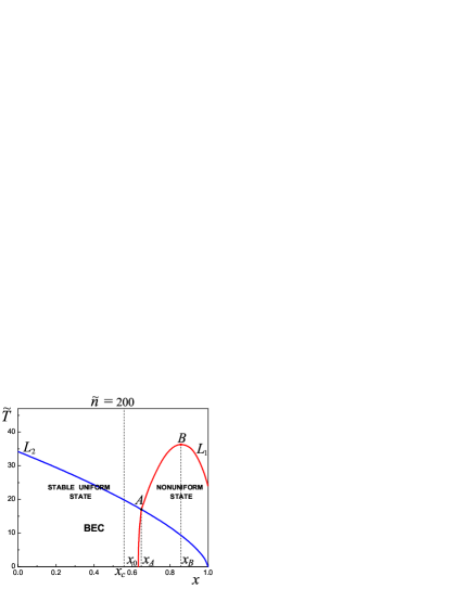
Figure 1: The diagram of stability of a mixture in the coordinates temperature – concentration at $\tilde{n}=200$:
$L_{1}$ – the boundary of the region of the stable uniform state,
$L_{2}$ – the condensation line $\tilde{T}_{C}(x)\equiv\tilde{n}^{2/3}(1-x)^{2/3}$, $x_{0}=0.63$, $A=(x_{A}=0.65,\tilde{T}_{A}=17.0)$ – the intersection point of $L_{1},L_{2}$, $B=(x_{B}=0.86,\tilde{T}_{B}=36.3)$ – the maximum point of $L_{1}$.

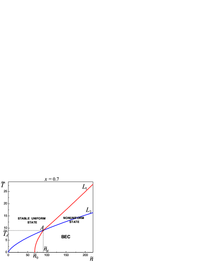
Figure 2: The diagram of stability of a mixture in the coordinates temperature – density at $x=0.7$:
$L_{1}$ – the boundary of the region of the stable uniform state,
$L_{2}$ – the condensation line $\tilde{T}_{C}(\tilde{n})\equiv\tilde{n}^{2/3}(1-x)^{2/3}$, $\tilde{n}_{0}=68.5$, $A=(\tilde{n}_{A}=90.5,\tilde{T}_{A}=9.03)$ – the intersection point of $L_{1},L_{2}$.

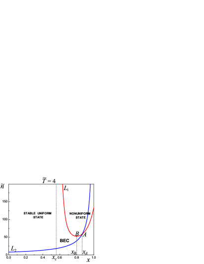
Figure 3: The diagram of stability of a mixture in the coordinates density – concentration at $\tilde{T}=4.0$:
$L_{1}$ – the boundary of the region of the stable uniform state,
$L_{2}$ – the condensation line $\tilde{n}_{C}(x)=\tilde{T}^{3/2}\!\big{/}(1-x)$,
$A=(x_{A}=0.86,\tilde{n}_{A}=58.5)$ – the intersection point of $L_{1},L_{2}$,
$B=(x_{B}=0.80,\tilde{n}_{B}=52.7)$ – the minimum point of $L_{1}$.

In Fig. 1 is shown the diagram of stability of a mixture in the coordinates $(x,\tilde{T})$. At the concentrations lower than $x_{0}$ the spatially uniform state proves to be stable at all temperatures. At $x_{0}<x<x_{A}$ the uniform state without condensate is stable at all temperatures, and the state with condensate is stable only just below the condensation line and becomes unstable with decreasing temperature. At $x>x_{A}$ there is the region of stability of the state without condensate (above the line $L_{1}$ in Fig. 1), and the state with condensate is always unstable. With decreasing the density the region of instability diminishes and the point $x_{0}$ shifts to the right. Thus, at $\tilde{n}=100$ the concentration $x_{0}=0.67$.

In Fig. 2 is shown the diagram of stability in the coordinates $(\tilde{n},\tilde{T})$. At the low densities $\tilde{n}<\tilde{n}_{0}$ the spatially uniform state is stable at all temperatures. At $\tilde{n}_{0}<\tilde{n}<\tilde{n}_{A}$ the uniform state without condensate is also stable, and the state with condensate is stable just below the condensation line and loses stability with decreasing temperature. At $\tilde{n}>\tilde{n}_{A}$ the state with condensate is always unstable, and the state without condensate is stable at high temperatures (above the line $L_{1}$ in Fig. 2).

In Fig. 3 is shown the diagram of stability in the coordinates $(x,\tilde{n})$. At low concentrations $x<x_{c}$ the spatially uniform state is stable at all densities. At $x_{c}<x<x_{A}$ the state without condensate is stable, and the spatially uniform state loses stability with increasing the density. At $x>x_{A}$ the state with condensate is unstable and there is only the region of stability of the state without condensate at low densities (below the line $L_{1}$ in Fig. 3).

Thus, the stability of the spatially uniform state of a mixture improves with decreasing the density and the concentration and with increasing the temperature. At densities and concentrations lower than some critical values, which are determined by the magnitude of interactions, the system becomes stable at all temperatures.

In the particular case of zero temperature the stability of a Fermi-Bose mixture was analyzed in work Viverit .

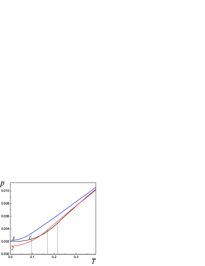
Figure 4: The dependencies of the total pressure $\tilde{p}=p/p_{*}$ $(p_{*}\equiv 4\pi\hbar^{2}\!\big{/}m_{B}l_{0}^{5})$ on the temperature $\tilde{T}$ at the density $\tilde{n}=0.1$ $(n=10^{17}\,\textrm{cm}^{-3})$ and various values of concentration $x$: (1) the pure Bose system $x=0$, $\tilde{T}_{C}=0.22$; (2) $x=0.3$, $\tilde{T}_{C}=0.17$; (3) $x=0.7$, $\tilde{T}_{C}=0.10$. The vertical dashed lines denote the condensation temperature.

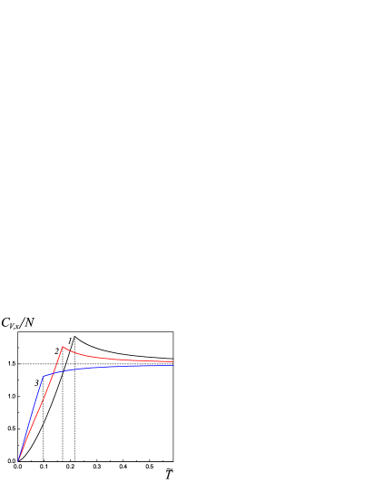
Figure 5: The temperature dependencies of the heat capacity at a constant volume at $\tilde{n}=0.1$ $(n=10^{17}\,\textrm{cm}^{-3})$ and various concentrations: (1) the pure Bose system $x=0$, $\tilde{T}_{C}=0.22$; (2) $x=0.3$, $\tilde{T}_{C}=0.17$; (3) $x=0.7$, $\tilde{T}_{C}=0.10$. The vertical dashed lines denote the condensation temperature.

Figure 6: The temperature dependencies of the heat capacity at a constant pressure at $\tilde{n}=0.1$ $(n=10^{17}\,\textrm{cm}^{-3})$ and various concentrations: (1) the pure Bose system $x=0$, $\tilde{T}_{C}=0.22$; (2) $x=0.3$, $\tilde{T}_{C}=0.17$; (3) $x=0.7$, $\tilde{T}_{C}=0.10$. The vertical dashed lines denote the condensation temperature.

VII Temperature dependencies of pressure, heat capacities and compressibilities

In this section we present the results of some numerical calculations based on the general formulas obtained in the previous sections for the equation of state, temperature dependencies of heat capacities, compressibilities and also the speed of sound. Being of the most interest, the behavior of thermodynamic quantities near the temperature of transition into the state with condensate can be analyzed if we take advantage of the expansions

$$\begin{array}[]{cc}\displaystyle{\Phi_{1/2}^{(-)}(t)\approx\!\sqrt{-\pi/t}+\zeta(1/2),\,\,\,\Phi_{3/2}^{(-)}(t)\approx\zeta(3/2)-2\sqrt{-\pi t},\vspace{4mm}}\\ \displaystyle{\Phi_{5/2}^{(-)}(t)\approx\zeta(5/2)+\zeta(3/2)\,t,}\end{array}$$ (85)

being valid for $|t|\ll 1$.

In Fig. 4 are presented the graphs of dependencies of the total pressure on temperature at a constant density and some concentrations. The pressure monotonically increases with increasing temperature. At the point of Bose-Einstein transition both the pressure and its first derivative remain continuous. Only the second derivative undergoes a jump $\Delta\big{(}\partial^{2}p\big{/}\partial T^{2}\big{)}\equiv\big{(}\partial^{2}p\big{/}\partial T^{2}\big{)}_{T_{C}+0}-\big{(}\partial^{2}p\big{/}\partial T^{2}\big{)}_{T_{C}-0}$ :

$$\begin{array}[]{ll}\displaystyle{\Delta\!\left(\!\frac{\partial^{2}p}{\partial T^{2}}\!\right)=-\frac{9}{8\pi}\frac{\big{[}\zeta(3/2)\big{]}^{3}}{T_{C}\big{[}\Lambda_{B}(T_{C})\big{]}^{3}}=\vspace{2mm}}\\ \displaystyle{\hskip 42.67912pt=-\frac{9}{8\pi}\big{[}\zeta(3/2)\big{]}^{3}\left(\frac{m_{B}}{2\pi\hbar^{2}}\right)^{\!3/2}T_{C}^{1/2}.}\end{array}$$ (86)

Since the condensation temperature decreases with increasing the concentration, then the value of the jump $\Delta\big{(}\partial^{2}p\big{/}\partial T^{2})$ decreases respectively. Note that the pressure of a mixture at $x=0.3$ (curve 2 in Fig. 4) at zero temperature proves to be lower than the pressure of a pure Bose system, which is conditioned by the attraction between fermions and between fermions and bosons.

The numerical calculation of the temperature dependencies of the heat capacities is presented in Figs. 5 and 6. In Fig. 5 are shown the temperature dependencies of the heat capacity per one particle at a constant volume for some values of the concentration. In a pure Bose system and at low concentrations the capacity at the condensation temperature has a sharp maximum (curves 1, 2), and at greater concentrations (curve 3) the maximum is absent but there remains the break. The form of the temperature dependencies of the isobaric heat capacity $C_{p,x}(\tilde{T})\big{/}N$, shown in Fig. 6, is qualitatively similar to the dependencies $C_{V,x}(\tilde{T})\big{/}N$, but the peaks at the condensation temperature at low concentrations prove to be more sharp.

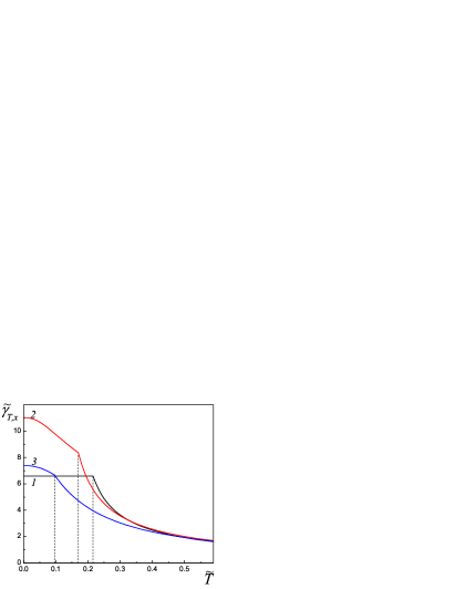
Figure 7: The temperature dependencies of the isothermal compressibility $\tilde{\gamma}_{T,x}=\gamma_{T,x}nT_{*}$ at $\tilde{n}=0.1$ $(n=10^{17}\,\textrm{cm}^{-3})$ and various concentrations: (1) the pure Bose system $x=0$, $\tilde{T}_{C}=0.22$; (2) $x=0.3$, $\tilde{T}_{C}=0.17$; (3) $x=0.7$, $\tilde{T}_{C}=0.10$. The vertical dashed lines denote the condensation temperature.

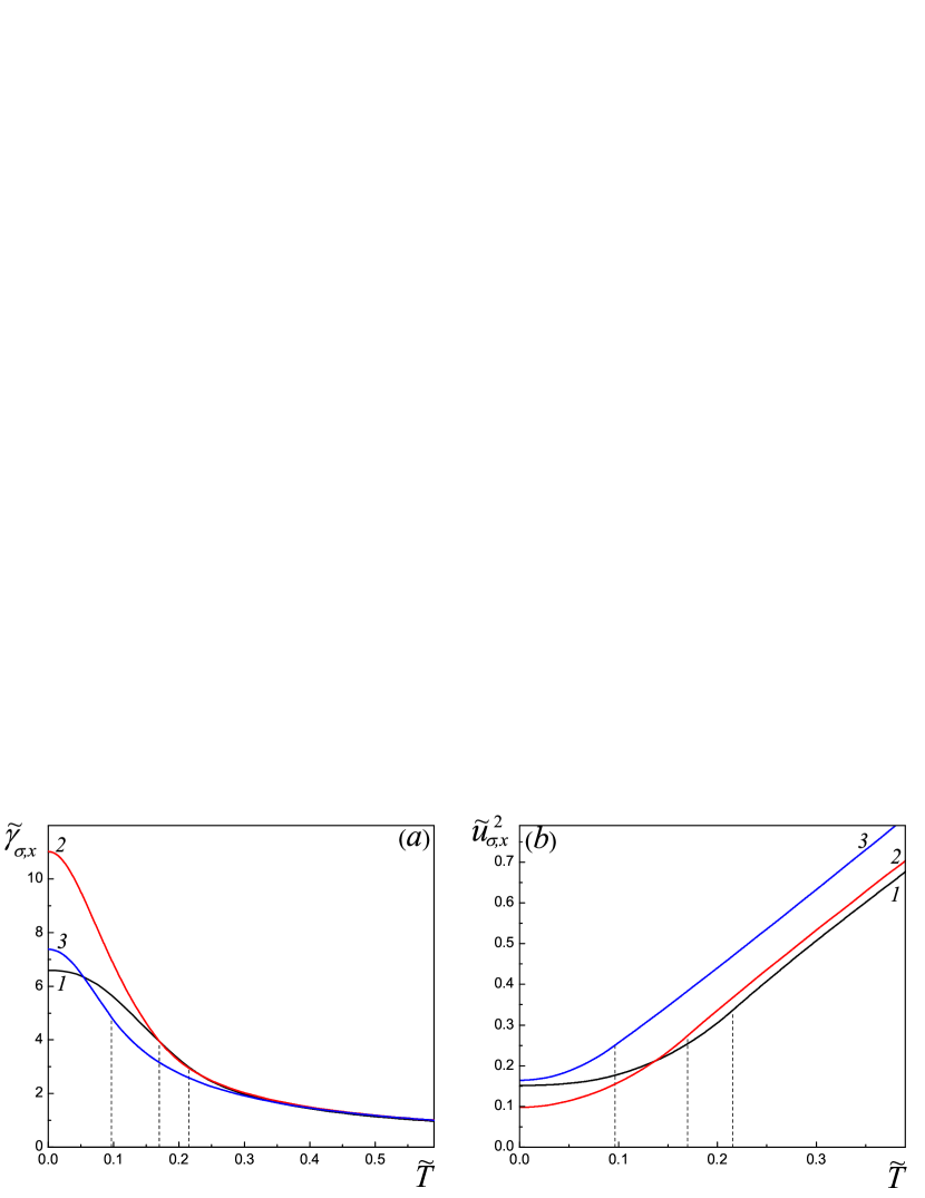
Figure 8: The temperature dependencies of (a) the adiabatic compressibility $\tilde{\gamma}_{\sigma,x}=\gamma_{\sigma,x}nT_{*}$ and (b) the square of speed of sound $\tilde{u}_{\sigma,x}^{2}=u_{\sigma,x}^{2}(m_{B}/T_{*})$ at $\tilde{n}=0.1$ $(n=10^{17}\,\textrm{cm}^{-3})$ and various concentrations: (1) the pure Bose system $x=0$, $\tilde{T}_{C}=0.22$; (2) $x=0.3$, $\tilde{T}_{C}=0.17$; (3) $x=0.7$, $\tilde{T}_{C}=0.10$. The vertical dashed lines denote the condensation temperature.

The decrease of the magnitudes of the heat capacity peaks at the condensation temperature as the concentration of fermions increases is qualitatively similar to what is observed in ³He – ⁴He solutions (see Eselson , ch. 2). Both heat capacities are continuous at the condensation temperature, but their derivatives at the transition from the high-temperature to the low-temperature phase undergo a jump $\Delta\big{(}\partial C\big{/}\partial T\big{)}\equiv\big{(}\partial C\big{/}\partial T\big{)}_{T_{C}+0}-\big{(}\partial C\big{/}\partial T\big{)}_{T_{C}-0}$ :

$$\vspace{04mm}\begin{array}[]{ll}\displaystyle{\Delta\!\left(\!\frac{\partial C_{V,x}}{\partial T}\!\right)=-(1-x)\frac{27}{16\pi}\zeta^{2}(3/2)\frac{N}{T_{C}}\,,\vspace{5mm}}\\ \displaystyle{\Delta\!\left(\!\frac{\partial C_{p,x}}{\partial T}\!\right)=-(1-x)\frac{27}{16\pi}\zeta^{2}(3/2)\frac{N}{T_{C}}\times\vspace{2mm}}\\ \displaystyle{\hskip 11.38109pt\times\!\left[\frac{\displaystyle{1+\frac{5}{6}\frac{nT_{C}}{G}x\frac{\Phi_{5/2}^{(+)}(t_{F0})}{\Phi_{3/2}^{(+)}(t_{F0})}+\!\frac{5}{6}\frac{nT_{C}}{G}(1-x)\frac{\zeta(5/2)}{\zeta(3/2)}}}{\displaystyle{1+\frac{nT_{C}}{2G}x\frac{\Phi_{3/2}^{(+)}(t_{F0})}{\Phi_{1/2}^{(+)}(t_{F0})}}}\right]^{2}\!.}\end{array}\vspace{00mm}$$ (87)

At $x=0$ these formulas, naturally, turn into the formulas of work P1 . In the limit of strong interaction $G\big{/}nT_{C}\gg 1$ the jumps of derivatives for both heat capacities (87) coincide. In the opposite limit of weak interaction $G\big{/}nT_{C}\ll 1$ the jump of the isobaric heat capacity proves to be independent of the interaction constants:

$$\begin{array}[]{ll}\displaystyle{\Delta\!\left(\!\frac{\partial C_{p,x}}{\partial T}\!\right)=-\frac{(1-x)}{x^{2}}\frac{27}{16\pi}\zeta^{2}(3/2)\frac{N}{T_{C}}\times\vspace{2mm}}\\ \displaystyle{\hskip 11.38109pt\times\!\left[\frac{5}{3}\frac{\Phi_{1/2}^{(+)}(t_{F0})}{\Phi_{3/2}^{(+)}(t_{F0})}\Bigg{(}\displaystyle{x\frac{\Phi_{5/2}^{(+)}(t_{F0})}{\Phi_{3/2}^{(+)}(t_{F0})}+(1-x)\frac{\zeta(5/2)}{\zeta(3/2)}}\Bigg{)}\right]^{2}\!.}\end{array}\vspace{06mm}$$ (88)

In this respect a mixture of Fermi and Bose particles differs from a pure Bose system, where at $G\rightarrow 0$ the heat capacity $C_{p}$ and the jump $\Delta\big{(}\partial C_{p}\big{/}\partial T\big{)}$ tend to infinity.

In Figs. 7 and 8 are shown the temperature dependencies of the isothermal and adiabatic compressibilities and the square of speed of sound. In a pure Bose system of interacting particles below the condensation temperature the isothermal compressibility proves to be independent of temperature (curve 1 in Fig. 7) P1 . The presence of the admixture of Fermi particles leads to the appearance of dependence of the isothermal compressibility on temperature in the state with condensate as well (curve 2, 3 in Fig. 7). At the condensation temperature the derivative with respect to temperature of the isothermal compressibility undergoes a jump:

$$\begin{array}[]{ll}\displaystyle{\Delta\!\left(\!\frac{\partial\gamma_{T,x}}{\partial T}\!\right)\!\!=\!-\frac{3n(1\!-x)\zeta^{2}\!(3/2)}{16\pi G^{2}}\Bigg{[}1\!+x\frac{nT_{C}}{2G}\frac{\Phi_{3/2}^{(+)}(t_{F0})}{\Phi_{1/2}^{(+)}(t_{F0})}\Bigg{]}^{\!-2}\!.}\end{array}\vspace{02mm}$$ (89)

The adiabatic compressibility and the speed of sound, as well as their first derivatives are continuous at the condensation temperatures (Fig. $8a,b$).

VIII Conclusion

In the paper, in general form for the pair potentials of the interparticle interaction, there are formulated the self-consistent field equations and obtained the thermodynamic relations for a mixture of Bose and Fermi particles. The case of a delta-like interaction between particles is studied in detail. Formulas for the thermodynamic potential, entropy, pressure, heat capacities at constant volume and pressure, isothermal and adiabatic compressibilities, speed of sound are obtained both above the temperature of Bose-Einstein condensation and in the state with condensate. The results of numerical calculations of these quantities as functions of temperature at different concentrations are presented. It is shown that with increasing the concentration of the admixture of Fermi particles, the temperature of Bose-Einstein condensation decreases and the features of thermodynamic quantities at the transition temperature, in particular of the heat capacity, become less pronounced. As in the case of a pure Bose system P1 , in the phase with condensate the dependence of thermodynamic quantities on the interaction constant between Bose particles proves to be nonanalytic, so that developing the perturbation theory in the interaction constant proves to be impossible here.

References

(1)
S.N. Bose, Plancks gesetz und lichtquanten hypothese, Z. Phys.
26 (1), 178 – 181 (1924).
doi: 10.1007/BF01327326
(2)
A. Einstein, Quantum theory of the monatomic ideal gas,
Sitzungsberichte der Preussischen Akademie der Wissenschaften,
Physikalisch-mathematische Klasse, 261 – 267, 1924; 3 – 14,
1925 [A. Einstein, A collection of scientific
works, Vol. 3, Nauka, Moscow, 481 – 511 (1966)]. doi: 10.1002/3527608958.ch27, 10.1002/3527608958.ch28
(3)
F. London, The - phenomenon of liquid helium and the
Bose-Einstein degeneracy, Nature 141, 643 (1938).
doi: 10.1038/141643a0
(4)
L. Tisza, Transport phenomena in helium II, Nature 141, 913 (1938). doi: 10.1038/141913a0
(5)
P.L. Kapitsa, Viscosity of liquid helium below the -point,
Nature 141, 74 (1938).
doi: 10.1038/141074a0
(6)
J.F. Allen, H. Jones, New phenomena connected with heat flow in
helium II, Nature 141, 234 (1938).
doi: 10.1038/141243a0
(7)
L. Landau, Theory of the superfluidity of helium II, J. Phys. USSR 5 (1), 71 (1941) [JETP 11, 592 (1941); paper 44 in: L. Landau, A collection of works, Vol. 1, Nauka, Moscow (1969)]. doi: 10.1103/PhysRev.60.356
(8)
A.D.B. Woods and R.A. Cowley, Structure and excitations of liquid helium, Rep. Progr. Phys. 36 (9), 1135 (1973).
doi: 10.1088/0034-4885/36/9/002
(14)
L. Landau, I. Pomeranchuk, On the motion of extraneous particles in helium II, DAN SSSR 59, 669 (1948) [paper 62 in: L. Landau, A collection of works, Vol. 2, Nauka, Moscow (1969)].
(15)
J. Bardeen, G. Baym, D. Pines, Effective interaction of 3He atoms in dilute solutions of 3He in 4He at low temperatures, Phys. Rev. 156, 207 (1967).
doi: 10.1103/PhysRev.156.207
(17)
M.Yu. Kagan, Fermi-gas approach to the problem of superfluidity in three- and two- dimensional solutions of 3He in 4He, Phys. Usp. 37, 69 (1994). doi: 10.3367/UFNr.0164.199401c.0077
(18)
A.V. Turlapov, Fermi gas of atoms, JETP Letters 95 (2), 96 (2012). doi: 10.1134/S0021364012020105
(19)
K.Mølmer, Bose condensates and Fermi gases at zero temperature,
Phys. Rev. Lett. 80, 1804 (1998).
doi: 10.1103/PhysRevLett.80.1804
(20)
T. Watanabe, T. Suzuki, P. Schuck, Bose-Fermi pair correlations in attractively interacting Bose-Fermi atomic mixtures, Phys. Rev. A 78, 033601 (2008).
doi: 10.1103/PhysRevA.78.033601
(21)
S.K. Adhikari, L. Salasnich, Superfluid Bose-Fermi mixture from weak coupling to unitarity, Phys. Rev. A 78, 043616 (2008).
doi: 10.1103/PhysRevA.78.043616
(22)
T. Maruyama, H. Yabu, Quadrupole oscillations in Bose-Fermi mixtures of ultracold atomic
gases made of Yb atoms in the time-dependent Gross-Pitaevskii and Vlasov equations, Phys. Rev. A 80, 043615 (2009).
doi: 10.1103/PhysRevA.80.043615
(23)
K. Noda, R. Peters, N. Kawakami, T. Pruschke, Many-body effects in a Bose-Fermi mixture, Phys. Rev. A 85, 043628 (2012).
doi: 10.1103/PhysRevA.85.043628
(24)
Y.M. Poluektov, A simple model of Bose-Einstein condensation of interacting particles, J. Low Temp. Phys. 186 (5–6), 347 (2017). doi: 10.1007/s10909-016-1715-5
(25)
Yu.M. Poluektov, Isobaric heat capacity of an ideal Bose gas, Russ. Phys. J. 44 (6), 627 (2001). doi: 10.1023/A:1012599929812
(28)
Yu.M. Poluektov, Self-consistent field model for spatially inhomogeneous Bose systems, Low Temp. Phys. 28 (6), 429 (2002). doi: 10.1063/1.1491184
(29)
Yu.M. Poluektov, On the quantum-field description of many-particle Fermi systems with spontaneously broken symmetry, Ukr. J. Phys. 50 (11), 1303 (2005); arXiv:1303.4913[cond-mat.stat-mech].
(30)
Yu.M. Poluektov, On the quantum-field description of many-particle Bose systems with spontaneously broken symmetry, Ukr. J. Phys. 52 (6), 579 (2007); arXiv:1306.2103[cond-mat.stat-mech].
(31)
Yu.M. Poluektov, A.A. Soroka, The equation of state and the quasiparticle mass
in the degenerate Fermi system with an effective interaction,
East Eur. J. Phys. 2 (3), 40 (2015); arXiv:1511.07682v1[cond-mat.stat-mech].
(32)
M.J. Jamieson, A. Dalgarno, M. Kimura, Scattering lengths and effective ranges
for He-He and spin-polarized H-H and D-D scattering,
Phys. Rev. A 51 (3), 2626 (1995). doi: 10.1103/PhysRevA.51.2626
(33)
L. Viverit, C.J. Pethick, H. Smith, Zero-temperature phase diagram of binary boson-fermion mixtures, Phys. Rev. A 61, 053605 (2000).
doi: 10.1103/Phys RevA.61.053605