Rates of multi-partite entanglement transformations and applications in quantum networks

Abstract

The theory of the asymptotic manipulation of pure bipartite quantum systems can be considered completely understood: The rates at which bipartite entangled states can be asymptotically transformed into each other are fully determined by a single number each, the respective entanglement entropy. In the multi-partite setting, similar questions of the optimally achievable rates of transforming one pure state into another are notoriously open. This seems particularly unfortunate in the light of the revived interest in such questions due to the perspective of experimentally realizing multi-partite quantum networks. In this work, we report substantial progress by deriving surprisingly simple upper and lower bounds on the rates that can be achieved in asymptotic multi-partite entanglement transformations. These bounds are based on ideas of entanglement combing and state merging. We identify cases where the bounds coincide and hence provide the exact rates. As an example, we bound rates at which resource states for the cryptographic scheme of quantum secret sharing can be distilled from arbitrary pure tripartite quantum states, providing further scope for quantum internet applications beyond point-to-point.

Entanglement is the feature of quantum mechanics that renders it distinctly different from a classical theory Horodecki et al. (2009). It is at the heart of quantum information science and technology as a resource that is used to accomplish task (and is increasingly also seen as an important concept in condensed-matter physics). Given its significance in protocols of quantum information, it hardly surprises that already early in the development of the field, questions were asked how one form of entanglement could be transformed into another. It was one of the early main results of the field of quantum information theory to show that all pure bipartite states could be asymptotically reversibly transformed to maximally entangled states with local operations and classical communication (LOCC) at a rate that is determined by a single number Bennett et al. (1996): the entanglement entropy, the von-Neumann entropy of each reduced state. This insight makes the resource character of bipartite entanglement most manifest: The entanglement content is given simply by its content of maximally entangled states, and each form can be transformed reversibly into another and back.

The situation in the multi-partite setting is significantly more intricate, however Walter et al. (2016); Bennett et al. (2000); de Vicente et al. (2017). The rates that can be achieved when aiming at asymptotically transforming one multi-partite state into another with LOCC are far from clear. It is not even understood what the “ingredients” of multi-partite entanglement theory are Bennett et al. (2000); Ishizaka and Plenio (2005), so the basic units of multi-partite entanglement from which any other pure state can be asymptotically reversibly prepared. This state of affairs is unfortunate, and even more so since multi-partite states come again more into the focus of attention in the light of the observation that elements of the vision of a quantum network – or the “quantum internet” Kimble (2008) – may become an experimental reality in the not too far future. It is not that multi-partite entanglement ceases to have a resource character: For example, Greenberger-Horne-Zeilinger (GHZ) states are known to constitute a resource for quantum secret sharing Hillery et al. (1999); Cleve et al. (1999), the probably best known multi-partite cryptographic primitive. Progress on stochastic conversion for several copies of multi-partite states was made recently Vrana and Christandl (2015, 2017). However, given a collection of arbitrary pure states, it is not known at what rate such states could be asymptotically distilled under LOCC.

In this work, we report surprisingly substantial progress on the old question of the rate at which GHZ and other multi-partite states can be asymptotically distilled from arbitrary pure states. Surprising, in that much of the technical substance can be delegated to the powerful machinery of entanglement combing Yang and Eisert (2009), putting it here into a fresh context, which in turn can be seen to derive from quantum state merging Horodecki et al. (2005, 2007), assisted entanglement distillation DiVincenzo et al. (1999); Smolin et al. (2005), and time-sharing, meaning, using resource states in different roles in the asymptotic protocol. The basic insight underlying the analysis is that entanglement combing provides a reference, a helpful normal form rooted in the better understood theory of bipartite entanglement, that can be used in order to assess rates of asymptotic multi-partite state conversion. Basically, putting entanglement combing to good work, therefore, we are in the position to make significant progress on the question of entanglement transformation rates in a general setting.

Multi-partite state conversion. We consider the problem of converting an $n$-partite state $\rho$ into $\sigma$ via $n$-partite LOCC. In particular, we are interested in the optimally achievable asymptotic rate for this procedure, which can be formally defined as

$$R(\rho\rightarrow\sigma)=\sup\left\{r:\lim_{k\rightarrow\infty}\left(\inf_{\Lambda}\left\|\Lambda\left(\rho^{\otimes k}\right)-\sigma^{\otimes\left\lfloor rk\right\rfloor}\right\|_{1}\right)=0\right\}.$$ (1)

Here, $\Lambda$ reflects an $n$-partite LOCC operation and $||M||_{1}=\mathrm{Tr}\sqrt{M^{\dagger}M}$ denotes the trace norm. This problem has a known solution in the bipartite case $n=2$ for conversion between arbitrary pure states $\psi^{AB}\rightarrow\phi^{AB}$, rooted in Shannon theory. The corresponding rate in this case can be written as Bennett et al. (1996)

$$R(\psi^{AB}\rightarrow\phi^{AB})=\frac{S(\psi^{A})}{S(\phi^{A})},$$ (2)

where $S(\rho)=-\mathrm{Tr}(\rho\log_{2}\rho)$ is the von Neumann entropy. Moreover, $\psi^{AB}$ indicates that the state is shared between parties referred to as Alice and Bob, while $\psi^{A}$ reflects the reduced state of Alice.

This simple picture ceases to hold in any setting beyond the bipartite one. Indeed, significantly less is known in the multi-partite setting for $n\geq 3$ Walter et al. (2016). Needless to say, the bipartite solution (2) readily gives upper bounds on the rates in multi-partite settings. For example, for conversion between tripartite pure states $\psi^{ABC}\rightarrow\phi^{ABC}$, it must be true that

$$R(\psi^{ABC}\rightarrow\phi^{ABC})\leq\min\left\{\frac{S(\psi^{A})}{S(\phi^{A})},\frac{S(\psi^{B})}{S(\phi^{C})},\frac{S(\psi^{C})}{S(\phi^{C})}\right\}.$$ (3)

This follows from the fact that any tripartite LOCC protocol is also bipartite with respect to any of the bipartitions. If the desired final state $\phi^{ABC}$ is the GHZ state with state vector $\ket{\mathrm{GHZ}}=(\ket{000}+\ket{111})/\sqrt{2}$, the bound in Eq. (3) is known to be achievable whenever one of the reduced states $\psi^{AB}$, $\psi^{BC}$ or $\psi^{AC}$ is separable Smolin et al. (2005).

We also note that for some states the bound in Eq. (3) is a strict inequality. This can be seen by considering the scenario where each of the parties holds two qubits respectively. Consider now the transformation

$$\begin{split}\ket{\mathrm{GHZ}}^{A_{1}B_{1}C_{1}}\otimes&\ket{\mathrm{GHZ}}^{A_{2}B_{2}C_{2}}\rightarrow\\ &\ket{\Phi^{+}}^{A_{1}B_{1}}\otimes\ket{\Phi^{+}}^{A_{2}C_{1}}\otimes\ket{\Phi^{+}}^{B_{2}C_{2}},\end{split}$$ (4)

i.e., the parties aim to transform two GHZ states into Bell states $\ket{\Phi^{+}}=(\ket{00}+\ket{11})/\sqrt{2}$ which are equally distributed among all the parties. It is straightforward to check that in this case the bound in Eq. (3) becomes $R\leq 1$. However, the bound is not achievable, as the aforementioned transformation cannot be performed with unit rate Linden et al. (2005).

Lower bound on conversion rates for three parties. The above discussion suggests that the bound in Eq. (3) is a very rough estimate for general transformations and is saturated only for very specific sets of states, having zero volume in the set of all pure states. Quite surprisingly, we will see below that this is not the case: there exist large families of tripartite pure states which saturate the bound (3). This will follow from a very general and surprisingly simple lower bound on conversion rate, which will be presented below in Theorem 2.

The methods developed here build upon the machinery of entanglement combing, which was introduced and studied for general $n$-partite scenarios in Ref. Yang and Eisert (2009). In the specific tripartite setting, entanglement combing aims to transform the initial state $\psi^{ABC}$ into a state of the form $\mu^{A_{1}B}\otimes\nu^{A_{2}C}$ with pure bipartite states $\mu$ and $\nu$. The following Lemma restates the results from Ref. Yang and Eisert (2009) in a form which will be suitable for the purpose of this work.

Lemma 1 (Conditions from tripartite entanglement combing).

The transformation

$$\psi^{ABC}\rightarrow\mu^{A_{1}B}\otimes\nu^{A_{2}C}$$ (5)

is possible via asymptotic LOCC if and only if

$$E(\mu^{A_{1}B})+E(\nu^{A_{2}C}) \leq S(\psi^{A}),$$ (6a)

$$E(\mu^{A_{1}B}) \leq S(\psi^{B}),$$ (6b)

$$E(\nu^{A_{2}C}) \leq S(\psi^{C}).$$ (6c)

We refer to Appendix A for the proof of the Lemma. Using this result, we are now in position to present a tight lower bound on the transformation rate between tripartite pure states.

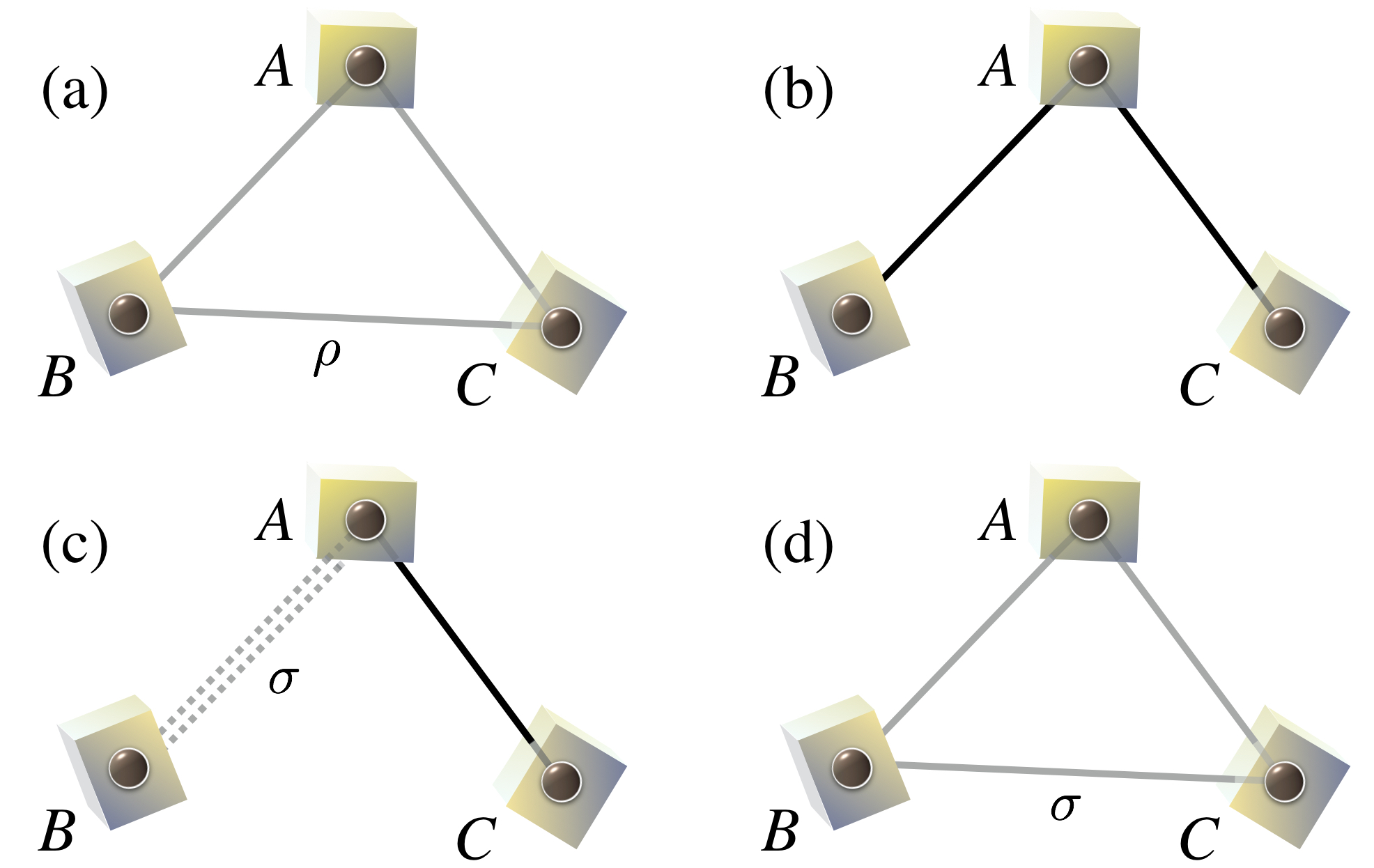
Figure 1: Conversion of a multi-partite resource state $\rho$ (a) into the desired final state $\sigma$ (d). The conversion is achieved via entanglement combing, i.e., via transforming the initial state $\rho$ into singlets [black solid lines in (b)]. One of the singlets is then converted into the desired final state $\sigma$ [gray dotted lines in (c)]. The remaining singlets [black solid line in (c)] are then used for teleporting the parts of $\sigma$ to the remaining parties.

Theorem 2 (Lower bound for state transformations).

For tripartite pure states $\psi^{ABC}$ and $\phi^{ABC}$, the LOCC conversion rate is bounded from below as

$$R(\psi^{ABC}\rightarrow\phi^{ABC})\geq\min\left\{\frac{S(\psi^{A})}{S(\phi^{B})+S(\phi^{C})},\frac{S(\psi^{B})}{S(\phi^{B})},\frac{S(\psi^{C})}{S(\phi^{C})}\right\}.$$ (7)

Proof.

We prove this bound by presenting an explicit protocol achieving the bound, which is also summarized in Fig. 1. In the first step, the parties apply entanglement combing $\psi^{ABC}\rightarrow\mu^{A_{1}B}\otimes\nu^{A_{2}C}$ in such a way that the following equalities are fulfilled for some $r\geq 0$,

$$E(\mu^{A_{1}B})=rS(\phi^{B}),\,\,\,\,\,\,\,\,E(\nu^{A_{2}C})=rS(\phi^{C}).$$ (8)

The significance of this specific choice will become clear in a moment. In the next step, Alice and Charlie apply LOCC for transforming the state $\nu^{A_{2}C}$ into the desired final state $\phi^{A_{2}A_{3}C}$. Since this is a bipartite LOCC protocol, the rate for this process is given by $E(\nu^{A_{2}C})/S(\phi^{C})$. Note that due to Eqs. (8), this rate is equal to $r$.

In a next step, Alice applies what is called Schumacher compression Schumacher (1995) to her register $A_{3}$. The overall compression rate per copy of the initial state $\psi^{ABC}$ is given as

$$\tilde{r}=rS(\phi^{A_{3}})=rS(\phi^{B}),$$ (9)

where in the last equality we used the fact that $S(\phi^{A_{3}})=S(\phi^{B})$. Due to Eqs. (8), this rate interestingly coincides with the entanglement of the state $\mu^{A_{1}B}$,

$$\tilde{r}=E(\mu^{A_{1}B}).$$ (10)

In a final step, Alice and Bob distill the states $\mu^{A_{1}B}$ into maximally entangled bipartite singlets, and use them to teleport Bennett et al. (1993); Pirandola et al. (2015) the (compressed) particle $A_{3}$ to Bob. Due to Eq. (10), Alice and Bob share exactly the right amount of entanglement for this procedure, i.e., the process is possible with rate one and no entanglement is left over. In summary, the overall protocol transforms the state $\psi^{ABC}$ into $\phi^{ABC}$ at rate $r$.

For completing the proof, we will now show that $r$ can be chosen such that

$$r=\min\left\{\frac{S(\psi^{A})}{S(\phi^{B})+S(\phi^{C})},\frac{S(\psi^{B})}{S(\phi^{B})},\frac{S(\psi^{C})}{S(\phi^{C})}\right\}.$$ (11)

This can be seen directly by inserting Eqs. (8) into Eqs. (6). In particular, the rate $r$ can attain any value which is simultaneously compatible with inequalities

$$r\leq\frac{S(\psi^{A})}{S(\phi^{B})+S(\phi^{C})},\,\,\,r\leq\frac{S(\psi^{B})}{S(\phi^{B})},\,\,\,r\leq\frac{S(\psi^{C})}{S(\phi^{C})}.$$ (12)

This completes the proof of the theorem. ∎

We stress some important aspects and implications of this theorem. Whenever the minimum in Eq. (7) is attained on the second or third entry, the lower bound coincides with the upper bound in Eq. (3). This means that in all these instances the conversion problem is completely solved, giving rise to the rate

$$R(\psi^{ABC}\rightarrow\phi^{ABC})=\min\left\{\frac{S(\psi^{A})}{S(\phi^{A})},\frac{S(\psi^{B})}{S(\phi^{B})},\frac{S(\psi^{C})}{S(\phi^{C})}\right\}.$$ (13)

Moreover, the bound in Eq. (7) can be immediately generalized by interchanging the roles of the parties, i.e.,

$$\begin{split}R(\psi^{ABC}\rightarrow\phi^{ABC})\geq&\min\left\{\frac{S(\psi^{B})}{S(\phi^{A})+S(\phi^{C})},\frac{S(\psi^{A})}{S(\phi^{A})},\frac{S(\psi^{C})}{S(\phi^{C})}\right\},\end{split}$$ (14)

$$\begin{split}R(\psi^{ABC}\rightarrow\phi^{ABC})\geq&\min\left\{\frac{S(\psi^{C})}{S(\phi^{A})+S(\phi^{B})},\frac{S(\psi^{A})}{S(\phi^{A})},\frac{S(\psi^{B})}{S(\phi^{B})}\right\}.\end{split}$$ (15)

The best bound is obtained by taking the maximum of Eqs. (7), (14) and (15).

Our results also shed new light on reversibility questions for tri-partite state transformations. In general, a transformation $\psi\rightarrow\phi$ is said to be reversible if the conversion rates fulfill the relation

$$R(\psi\rightarrow\phi)={R(\phi\rightarrow\psi)}^{-1}.$$ (16)

Let now $\psi$ and $\phi$ be two states for which the bound in Theorem 2 is tight, e.g., $R(\psi\rightarrow\phi)=S(\psi^{A})/S(\phi^{A})$. Due to Eq. (3) it must be that $S(\psi^{A})/S(\phi^{A})\leq S(\psi^{B})/S(\phi^{B})$ in this case. If this inequality is strict (which will be the generic case), we obtain for the inverse transformation $\phi\rightarrow\psi$

$$R(\phi\rightarrow\psi)\leq\frac{S(\phi^{B})}{S(\psi^{B})}<\frac{S(\phi^{A})}{S(\psi^{A})}={R(\psi\rightarrow\phi)}^{-1},$$ (17)

where the first inequality follows from Eq. (3). These results show that those states which saturate the bound (3) do not allow for reversible transformations in the generic case.

We will now comment on the limits of the approach presented here. In particular, it is important to note that the lower bound in Theorem 2 is not optimal in general. This can be seen in the most simple way by considering the trivial transformation which leaves the state unchanged, i.e., $\psi^{ABC}\rightarrow\psi^{ABC}$. Clearly, this can be achieved with unit rate $R=1$. However, if we apply the lower bound in Theorem 2 to this transformation, we get $R\geq{S(\psi^{A})}/[S(\psi^{B})+S(\psi^{C})]$. Due to subadditivity, it follows that that our lower bound is in general below the achievable unit rate in this case.

Multi-partite pure states. In the discussion so far, we have focused on tripartite pure states. However, the presented tools can readily be applied to more general scenarios involving an arbitrary number of parties. In this more general setup the parties will be called Alice $(A)$ and $N$ Bobs $(B_{i})$ with $1\leq i\leq N$. The aim of the process in this case is the asymptotic conversion of the $N+1$-partite pure state $\psi=\psi^{AB_{1}\ldots B_{N}}$ into the state $\phi=\phi^{AB_{1}\ldots B_{N}}$. The general idea for this procedure follows the same line of reasoning as in the tripartite scenario discussed above. In the first step, entanglement combing is applied to the state $\psi$, i.e., the transformation

$$\psi\rightarrow\mu_{1}^{A_{1}B_{1}}\otimes\mu_{2}^{A_{2}B_{2}}\otimes\cdots\otimes\mu_{N}^{A_{N}B_{N}}$$ (18)

with pure states $\mu_{i}$. In the next step, Alice and the first Bob $B_{1}$ transform their state $\mu_{1}^{A_{1}B_{1}}$ into the desired final state $\phi$ via bipartite LOCC. In the final step, Alice applies Schumacher compression to parts of her state $\phi$, and sends these parts to each of the remaining Bobs $B_{2},\ldots,B_{N}$ by using entanglement obtained in the first step of this protocol. As in the tripartite case, this protocol can be further optimized by interchanging the roles of the parties and applying the time-sharing technique.

Theorem 3 (Lower bound for multi-partite state conversion).

For $N+1$-partite pure states $\psi^{AB_{1}\dots B_{N}}$ and $\phi^{AB_{1}\dots B_{N}}$, the LOCC conversion rate is bounded from below as

$$R(\psi^{AB_{1}\dots B_{N}}\rightarrow\phi^{AB_{1}\dots B_{N}})\geq\min_{X}\left\{\frac{S(\psi^{AX})}{\sum_{B_{i}\notin X}S(\phi^{B_{i}})}\right\},$$ (19)

where $X$ denotes a subsystem of all Bobs.

The theorem is proven in Appendix B. By using similar arguments as below Eq. (3), an upper bound to the conversion rate is found to be

$$R(\psi^{AB_{1}\dots B_{N}}\rightarrow\phi^{AB_{1}\dots B_{N}})\leq\min_{i}\frac{S(\psi^{B_{i}})}{S(\phi^{B_{i}})}.$$ (20)

The bounds in Eqs. (19) and (20) coincide if the following equality holds true for some $1\leq i\leq N$,

$$\frac{S(\psi^{B_{i}})}{S(\phi^{B_{i}})}=\min_{X}\left\{\frac{S(\psi^{AX})}{\sum_{B_{j}\notin X}S(\phi^{B_{j}})}\right\}.$$ (21)

In those instances, Theorem 3 leads to a full solution of the conversion problem, and the corresponding rate is given by

$$R(\psi^{AB_{1}\dots B_{N}}\rightarrow\phi^{AB_{1}\dots B_{N}})=\min_{i}\frac{S(\psi^{B_{i}})}{S(\phi^{B_{i}})}.$$ (22)

Again, as in the tripartite case, the bound of Eq. (19) can be generalized by interchanging the roles of Alice and different Bobs.

Generalization to multi-partite mixed states. We will now show that the ideas which led to lower bounds on conversion rates in the previous sections can also be used in this mixed-state scenario. We will demonstrate this on a specific example, considering the transformation

$$\ket{\mathrm{GHZ}}\!\bra{\mathrm{GHZ}}\rightarrow\sigma,$$ (23)

where $\ket{\mathrm{GHZ}}=(\ket{0}^{\otimes N+1}+\ket{1}^{\otimes N+1})/\sqrt{2}$ denotes an $N+1$-partite GHZ state vector, and $\sigma=\sigma^{AB_{1}\ldots B_{N}}$ is an arbitrary $N+1$-partite mixed state. As we show in Appendix E, by using similar methods as in previous sections, we obtain a lower bound on the transformation rate,

$$R(\ket{\mathrm{GHZ}}\!\bra{\mathrm{GHZ}}\ \rightarrow\sigma)\geq\frac{1}{E_{\mathrm{c}}^{A|B_{1}\ldots B_{N}}(\sigma)+\sum_{j=3}^{N}S(\sigma^{B_{j}})},$$ (24)

where $E_{\mathrm{c}}^{A|B_{1}\ldots B_{N}}$ denotes the entanglement cost Hayden et al. (2001) between Alice and all the other Bobs.

The upper bound (20) for the transformation rate $R$ can be generalized as (see Eq. (146) in Ref. Horodecki et al. (2009))

$$R(\rho\rightarrow\sigma)\leq\min_{\mathcal{P}}\frac{E_{\infty}^{\mathcal{P}|\overline{\mathcal{P}}}(\rho)}{E_{\infty}^{\mathcal{P}|\overline{\mathcal{P}}}(\sigma)}.$$ (25)

Here, $E_{\infty}(\rho)=\lim_{n\rightarrow\infty}E_{\mathrm{r}}(\rho^{\otimes n})/n$ is the regularized relative entropy of entanglement Audenaert et al. (2001); Winter (2016), and $\mathcal{P}|\overline{\mathcal{P}}$ denotes a bipartition of all the $N+1$ subsystems .

Applications in quantum networks. It should be clear that the results established here readily allow to assess how resources for multi-partite protocols can be prepared from multi-partite states given in some form. In particular, GHZ states readily provide a resource for quantum secret sharing Hillery et al. (1999); Cleve et al. (1999) in which a message is split into parts so that no subset of parties is able to access the message, while at the same time the entire set of parties is. It also gives rise to an efficient scheme of quantum secret sharing requiring purely classical communication during the reconstruction phase Broadbent et al. (2009).

The significance in the established results on multi-partite entanglement transformations hence lies in the way they help understanding how multi-partite resources for protocols beyond point-to-point schemes in quantum networks can be prepared and manipulated. We expect this to be particularly important when thinking of applications of transforming resources into the desired form in quantum networks Schoute et al. ; Dahlberg and Wehner (0325); Hahn et al. (2019): Here, multi-partite entanglement is conceived to be created by local processes and bi-partite transmissions involving pairs of nodes, followed by steps of entanglement manipulation, which presumably involve instances of classical routing techniques. Hence, we see this work as a significant contribution to how a quantum internet Kimble (2008) can possibly be conceived.

Conclusions. In this work, we have reported substantial progress on asymptotic state transformation via multipartite local operations and classical communication, tackling an important long-standing problem which to large extent remained open since the early development of quantitative entanglement theory Bennett et al. (2000). Similar techniques may also prove helpful in the study of other quantum resource theories different from entanglement, such as the resource theory of quantum coherence Streltsov et al. (2017) and quantum thermodynamics Lostaglio et al. (2015); Ćwikliński et al. (2015).

Putting notions of entanglement combing into a fresh light, we have been able to derive stringent bounds on multi-partite entanglement transformations. This progress seems particularly relevant in the light of the advent of quantum networks and the quantum internet in which multi-partite features are directly exploited beyond point-to-point architectures. It is the hope that the present work stimulates further progress in the understanding of multi-partite protocols.

Acknowledgements. We acknowledge discussions with Paweł Horodecki and financial support by the Alexander von Humboldt-Foundation, the National Science Center in Poland (POLONEZ UMO-2016/21/P/ST2/04054), the BMBF (Q.com, Q.Link.X), and the ERC (TAQ). This work was further supported by the "Quantum Coherence and Entanglement for Quantum Technology" project, carried out within the First Team programme of the Foundation for Polish Science co-financed by the European Union under the European Regional Development Fund.

Appendix A Proof of Lemma 1

The proof presented below will be based on the protocol known as entanglement combing Yang and Eisert (2009). We will review this protocol for a tripartite state $\psi=\psi^{ABC}$. In this case, entanglement combing transforms the state $\psi^{ABC}$ into $\mu^{A_{1}B}\otimes\nu^{A_{2}C}$ with pure states $\mu$ and $\nu$. Clearly, the transformation is not possible if any of the inequalities (6) is violated. We will now show the converse, i.e., any pair of pure states $\mu^{A_{1}B}$ and $\nu^{A_{2}C}$ which fulfill the inequalities (6) can be obtained from $\psi^{ABC}$ via LOCC in the asymptotic limit. For this, we will distinguish between the following cases.

Case 1: $S(\psi^{A})\geq S(\psi^{B})\geq S(\psi^{C})$. In this case, Bob can send his part of the state $\psi$ to Alice by applying quantum state merging Horodecki et al. (2005, 2007). This procedure is possible by using LOCC operations between Alice and Bob. Additionally, Alice and Bob gain singlets at rate $S(\psi^{A})-S(\psi^{AB})=S(\psi^{A})-S(\psi^{C})$. The overall process thus achieves the transformation (5) with

$$E(\mu^{A_{1}B}) =S(\psi^{A})-S(\psi^{C}),$$ (26)

$$E(\nu^{A_{2}C}) =S(\psi^{C}).$$

Alternatively, Charlie can send his part of the state $\psi$ to Alice, thus gaining singlets at rate $S(\psi^{A})-S(\psi^{B})$. In this way they achieve the transformation (5) with

$$E(\mu^{A_{1}B}) =S(\psi^{B}),$$ (27)

$$E(\nu^{A_{2}C}) =S(\psi^{A})-S(\psi^{B}).$$

In the next step we apply-time sharing, i.e., the first procedure is performed with probability $p$ and the second with probability $(1-p)$. In this way, we see that the transformation (5) is possible for any pair of states $\mu^{A_{1}B}$ and $\nu^{A_{2}C}$ with the property

$$E(\mu^{A_{1}B}) =p\left(S(\psi^{A})-S(\psi^{C})\right)+(1-p)S(\psi^{B}),$$ (28)

$$E(\nu^{A_{2}C}) =pS(\psi^{C})+(1-p)\left(S(\psi^{A})-S(\psi^{B})\right).$$

By using subadditivity of von Neumann entropy it is now straightforward to check that for a suitable choice of $p$, the quantities $E(\mu^{A_{1}B})$ and $E(\nu^{A_{2}C})$ can attain any value compatible with conditions

$$E(\mu^{A_{1}B})+E(\nu^{A_{2}C}) =S(\psi^{A}),$$ (29a)

$$E(\mu^{A_{1}B}) \leq S(\psi^{B}),$$ (29b)

$$E(\nu^{A_{2}C}) \leq S(\psi^{C}).$$ (29c)

This completes the proof of Lemma 1 for Case 1.

Case 2: $S(\psi^{B})\geq S(\psi^{C})\geq S(\psi^{A})$. In this case, Alice, Bob, and Charlie apply assisted entanglement distillation DiVincenzo et al. (1999); Smolin et al. (2005), with Charlie being the assisting party. This procedure achieves the transformation (5) with

$$E(\mu^{A_{1}B}) =\min\left\{S(\psi^{A}),S(\psi^{B})\right\}=S(\psi^{A}),$$ (30)

$$E(\nu^{A_{2}C}) =0.$$

Alternatively, they can apply assisted entanglement distillation with Bob being the assisting party, thus achieving

$$E(\mu^{A_{1}B}) =0,$$ (31)

$$E(\nu^{A_{2}C}) =\min\left\{S(\psi^{A}),S(\psi^{C})\right\}=S(\psi^{A}).$$

By applying time-sharing, we see that we can achieve the transformation (5) with any states $\mu^{A_{1}B}$ and $\nu^{A_{2}C}$ fulfilling

$$E(\mu^{A_{1}B}) =pS(\psi^{A}),$$ (32a)

$$E(\nu^{A_{2}B}) =(1-p)S(\psi^{A}).$$ (32b)

This completes the proof of Lemma 1 for Case 2.

Case 3: $S(\psi^{B})\geq S(\psi^{A})\geq S(\psi^{C})$. Here, we will apply a combination of protocols used in Case 1 and 2. In particular, Bob can send his part of the state $\psi$ to Alice by quantum state merging, see Eq. (26). Alternatively, they can apply assisted entanglement distillation, see Eq. (30). By time-sharing we obtain

$$E(\mu^{A_{1}B}) =S(\psi^{A})-pS(\psi^{C}),$$ (33)

$$E(\nu^{A_{2}C}) =pS(\psi^{C}).$$

By a suitable choice of the probability $p$ it is now possible to obtain any pair of states $\mu^{A_{1}B}$ and $\nu^{A_{2}C}$ such that

$$E(\mu^{A_{1}B})+E(\nu^{A_{2}C}) =S(\psi^{A}),$$ (34)

$$E(\mu^{A_{1}B}) \leq S(\psi^{A}),$$

$$E(\nu^{A_{2}C}) \leq S(\psi^{C}).$$

This completes the proof of Lemma 1 for Case 3. Note that any other case can be obtained from the above three cases by interchanging the role of Bob and Charlie. Thus, the proof of the Lemma is complete.

Appendix B Proof of Theorem 3

Here, we present the proof of Theorem 3. The ideas presented in the following generalize the proof of Theorem 2 for tripartite pure state conversion. In particular, starting with the $N+1$-partite state $\psi=\psi^{AB_{1}\dots B_{N}}$, we will apply entanglement combing Yang and Eisert (2009) on Alice and all other parties (here referred to as “all the Bobs”), aiming to get bipartite entanglement between Alice and each of the parties $B_{i}$. If $E_{i}$ denotes the entanglement between Alice and $i$-th Bob after this procedure, the rate for state conversion from $\psi$ to $\phi=\phi^{AB_{1}\dots B_{N}}$ is bounded below as

$$R(\psi\rightarrow\phi)\geq\min_{i}\left\{\frac{E_{i}}{S(\phi^{B_{i}})}\right\}.$$ (35)

To achieve conversion at rate $\min_{i}\left\{E_{i}/S(\phi^{B_{i}})\right\}$, Alice locally prepares the state $\phi^{A\tilde{A}_{1}\dots\tilde{A}_{N}}$, applies Schumacher compression Schumacher (1995) to the registers $\tilde{A}_{i}$, and distributes them among the Bobs by using entanglement which has been combed in the previous procedure. In the rest of this section, we will show that combing can achieve an $N$-tuple of singlet rates $(E_{1},\dots,E_{N})$ such that

$$\min_{i}\left\{\frac{E_{i}}{S(\phi^{B_{i}})}\right\} \geq m^{\psi,\phi}:=\min_{X}\left\{\frac{S(\psi^{AX})}{\sum_{B_{i}\notin X}S(\phi^{B_{i}})}\right\},$$ (36)

where $X$ denotes a subset of all the Bobs. When there is no ambiguity, we will denote $m^{\psi,\phi}$ simply by $m$.

In the first step of the proof we will consider all possible ways to merge Bobs’ parts of the state $B_{i}$ with Alice. Since in the scenario considered here we have $N$ Bobs, there are $N!$ different ways to achieve this, depending on the order of the Bobs in the merging procedure. We will first consider entanglement $N$-tuple $(E_{1},\dots,E_{N})$, where $E_{i}$ denotes the amount of entanglement shared between Alice and $i$-th Bob after the merging procedure. For example, taking $N=4$, merging first $B_{1}$, then $B_{2}$, then $B_{3}$ and finally $B_{4}$ to Alice will achieve the $4$-tuple:

$$E_{1} =S(\psi^{A})-S(\psi^{AB_{1}}),$$ (37a)

$$E_{2} =S(\psi^{AB_{1}})-S(\psi^{AB_{1}B_{2}}),$$ (37b)

$$E_{3} =S(\psi^{AB_{1}B_{2}})-S(\psi^{AB_{1}B_{2}B_{3}}),$$ (37c)

$$E_{4} =S(\psi^{AB_{1}B_{2}B_{3}}),$$ (37d)

while merging first $B_{3}$, then $B_{1}$, then $B_{4}$ and finally $B_{2}$ to Alice will achieve the $4$-tuple:

$$E_{1} =S(\psi^{AB_{3}})-S(\psi^{AB_{1}B_{3}}),$$ (38a)

$$E_{2} =S(\psi^{AB_{1}B_{3}B_{4}}),$$ (38b)

$$E_{3} =S(\psi^{A})-S(\psi^{AB_{3}}),$$ (38c)

$$E_{4} =S(\psi^{AB_{1}B_{3}})-S(\psi^{AB_{1}B_{3}B_{4}}).$$ (38d)

The aforementioned $N!$ merging procedures give rise to $N!$ $N$-tuples, which we will name the "entanglement extreme points". We note that some of the values $E_{i}$ can be negative, implying that entanglement is consumed in this case. Proposition 2 of Ref. Yang and Eisert (2009) guarantees that for any $N$-tuple $(E_{1},\dots,E_{N})$ with the properties

1. $\forall i\in\{1,\dots,N\}$, $E_{i}\geq 0$,

2. $(E_{1},\dots,E_{N})$ is in the convex polytope spanned by the entanglement extreme points,

there exists an asymptotic LOCC protocol acting on the state $\psi$ and distilling singlets between Alice and each of the Bobs $B_{i}$ at rate $E_{i}$. In the following, we are interested in the renormalized entanglement rates

$$R_{i}=\frac{E_{i}}{S(\phi^{B_{i}})},$$ (39)

see also Eq. (35). We can define for each $N$-tuple $(E_{1},\dots,E_{N})$ an $N$-tuple $(R_{1},\dots,R_{N})$. We will consider from now on only the tuples $(R_{1},\dots,R_{N})$, which will also be called "rate distributions". We will call "extreme points" the rates distribution defined from the entanglement extreme points. It is easily seen from previous combing condition and Eq. (35) that, if we find a distribution of rates $(R_{1},\dots,R_{N})$ satisfying

1. $\forall i\in\{1,\dots,N\}$, $R_{i}\geq 0$,

2. $(R_{1},\dots,R_{N})$ is in the convex polytope spanned by the extreme points,

we will be able to achieve conversion from $\psi$ to $\phi$ with rate

$$R(\psi\rightarrow\phi)\geq\min_{i}\left\{R_{i}\right\}.$$ (40)

In order to prove Eq. (36), we will find in the convex set of the extreme points a point $(R_{1},\dots,R_{N})$ such that

$$\min_{i}\left\{R_{i}\right\} \geq\min_{X}\left\{\frac{S(\psi^{AX})}{\sum_{B_{i}\notin X}S(\phi^{B_{i}})}\right\}.$$ (41)

The outline of the rest of the proof is as follows: in the first step we will construct by convexity a set of points $(R_{1},\dots,R_{N})$ satisfying $R_{N}\geq m^{\psi,\phi}$ from the extreme points. We note that the convex set of these newly constructed points will only contain rate distributions with $N^{\textrm{th}}$ coordinate superior to $m^{\psi,\phi}$. From our constructed points, we will construct by convexity a new set of points $(R_{1},\dots,R_{N})$ satisfying $R_{N-1}\geq m^{\psi,\phi}$. This will lead to a set of point satisfying both $R_{N}\geq m^{\psi,\phi}$ and $R_{N-1}\geq m^{\psi,\phi}$. The procedure will continue with $R_{N-2}$ until $R_{1}$. In this way, we will achieve a distribution $(R_{1},\dots,R_{N})$ satisfying $\forall i\in\{1,\dots,N\},R_{i}\geq m^{\psi,\phi}$. Such a distribution will ensure conversion from $\psi$ to $\phi$ with a rate of at least $m^{\psi,\phi}$, as claimed.

First step. Each of the extreme points is the result of merging the Bobs to Alice in different order. Thus, we can associate each extreme point to a permutation $\sigma$ on the set $\{1,\dots,N\}$. We denote the set of all permutations by $\mathcal{S}_{N}$. Moreover, $\sigma(k)=l$ means that $B_{l}$ is the $k^{\textrm{th}}$ Bob merged to Alice. It implies that,

$$R_{\sigma(k)}^{\sigma}=R_{l}^{\sigma} =\frac{S(\psi^{AB_{\sigma(1)}\dots B_{\sigma(k-1)}})-S(\psi^{AB_{\sigma(1)}\dots B_{\sigma(k-1)}B_{l}})}{S(\phi^{B_{l}})}$$

$$=\frac{S(\psi^{AY^{\sigma}_{k-1}})-S(\psi^{AY^{\sigma}_{k-1}B_{l}})}{S(\phi^{B_{l}})},$$ (42)

where we used the notation $Y^{\sigma}_{k}=\{B_{\sigma(1)},\dots,B_{\sigma(k)}\}$.

Our next observation is that we can group the $N!$ extreme points in $(N-1)!$ sets of $N$ points. In the following, we denote by $c_{N-i}$ the permutations defined for $i\in\{0,\dots,N-1\}$ as

$$c_{N-i}(k) =k\textrm{, }\forall k\in\{1,\dots,N-i-1\},$$ (43a)

$$c_{N-i}(N-i) =N,$$ (43b)

$$c_{N-i}(k) =k-1\textrm{, }\forall k\in\{N-i+1,\dots,N\}.$$ (43c)

Consider now a distribution $(R_{1}^{\sigma},\dots,R_{N}^{\sigma})$ with $\sigma(N)=N$, i.e., $B_{N}$ merged in $N^{\textrm{th}}$ position. We form a set by grouping together the $N$ distributions $(R_{1}^{\sigma\circ c_{N-i}},\dots,R_{N}^{\sigma\circ c_{N-i}})$. In term of merging order, the distribution $\sigma\circ c_{N-i}$ give rise to the following ordering:

1. For $k<N-i$, $B_{\sigma\circ c_{N-i}(k)}=B_{\sigma(k)}$ is merged in position $k$,

2. For $k=N-i$, $B_{\sigma\circ c_{N-i}(N-i)}=B_{N}$ is merged in position $N-i$,

3. For $N\geq k>N-i$, $B_{\sigma\circ c_{N-i}(k)}=B_{\sigma(k-1)}$ is merged in position $k$.

Distributions $\sigma\circ c_{N-i}$ are the distributions obtained by merging Bobs $1$ to $N-1$ with the relative order given by $\sigma$. The only difference is the merging position of $B_{N}$.

We can order this set by the value of the $N^{\textrm{th}}$ coordinate. Indeed,

$$R_{N}^{\sigma}\geq R_{N}^{\sigma\circ c_{N-1}}\geq R_{N}^{\sigma\circ c_{N-2}}\geq\dots\geq R_{N}^{\sigma\circ c_{1}}.$$ (44)

Note that $\sigma\circ c_{N}=\sigma$. For a proof of Eq. (44) in the general case see Appendix C. There are $(N-1)!$ distributions satisfying $\sigma(N)=N$. We have $(N-1)!$ ordered sets of size $N$. Observe that for all $\sigma\in S_{N}$ satisfying $\sigma(N)=N$,

$$R_{N}^{\sigma}=\frac{S(\psi^{AB_{1}\dots B_{N-1}})}{S(\phi^{B_{N}})}\in\left\{\frac{S(\psi^{AX})}{\sum_{B_{i}\notin X}S(\phi^{B_{i}})}\right\}$$ (45)

As a consequence,

$$R_{N}^{\sigma}\geq m^{\psi,\phi}.$$ (46)

Two situations can happen for each of the $(N-1)!$ sets. The first case is that $R_{N}^{\sigma\circ c_{1}}\geq m^{\psi,\phi}$. In this case, we can obtain the distribution $(R_{1}^{\sigma\circ c_{1}},\dots,R_{N-1}^{\sigma\circ c_{1}},m^{\psi,\phi})$ from $(R_{1}^{\sigma\circ c_{1}},\dots,R_{N}^{\sigma\circ c_{1}})$ by simply reducing the entanglement between Alice and $B_{N}$.

The second case is that we can find $i$ such that $R_{N}^{\sigma\circ c_{N-i}}\geq m^{\psi,\phi}>R_{N}^{\sigma\circ c_{N-i-1}}$. In this case, we can consider a convex combination of $R^{\sigma\circ c_{N-i}}$ and $R^{\sigma\circ c_{N-i-1}}$, in order to arrive at a resulting distribution $(R_{1},\dots,R_{N})$ such that $R_{N}=m^{\psi,\phi}$. We also know easily the value of most of the two distribution’s coordinates. Indeed,

1. For $k<N-i-1$, $c_{N-i-1}(k)=c_{N-i}(k)=k$, which gives

   $$R^{\sigma\circ c_{N-i-1}}_{\sigma\circ c_{N-i-1}(k)}= R^{\sigma\circ c_{N-i-1}}_{\sigma(k)}=\frac{S(\psi^{AY^{\sigma}_{k-1}})-S(\psi^{AY^{\sigma}_{k}})}{S(\phi^{B_{\sigma(k)}})},$$ (47a)

   $$R^{\sigma\circ c_{N-i}}_{\sigma\circ c_{N-i}(k)}= R^{\sigma\circ c_{N-i}}_{\sigma(k)}=\frac{S(\psi^{AY^{\sigma}_{k-1}})-S(\psi^{AY^{\sigma}_{k}})}{S(\phi^{B_{\sigma(k)}})}.$$ (47b)

2. For $k=N-i-1$, $c_{N-i-1}(N-i-1)=N$ and $c_{N-i}(N-i-1)=N-i-1$,

   $$R^{\sigma\circ c_{N-i-1}}_{\sigma\circ c_{N-i-1}(N-i-1)}= R^{\sigma\circ c_{N-i-1}}_{N}=\frac{S(\psi^{AY_{N-i-2}^{\sigma}})-S(\psi^{AY_{N-i-2}^{\sigma}B_{N}})}{S(\phi^{B_{N}})},$$ (48a)

   $$R^{\sigma\circ c_{N-i}}_{\sigma\circ c_{N-i}(N-i-1)}= R^{\sigma\circ c_{N-i}}_{\sigma(N-i-1)}=\frac{S(\psi^{AY_{N-i-2}^{\sigma}})-S(\psi^{AY_{N-i-1}^{\sigma}})}{S(\phi^{B_{\sigma(N-i-1)}})}.$$ (48b)

3. For $k=N-i$, $c_{N-i-1}(N-i)=N-i-1$ and $c_{N-i}(N-i)=N$,

   $$R^{\sigma\circ c_{N-i-1}}_{\sigma\circ c_{N-i-1}(N-i)}= R^{\sigma\circ c_{N-i-1}}_{\sigma(N-i-1)}=\frac{S(\psi^{AY_{N-i-2}^{\sigma}B_{N}})-S(\psi^{AY_{N-i-1}^{\sigma}B_{N}})}{S(\phi^{B_{\sigma(N-i-1)}})},$$ (49a)

   $$R^{\sigma\circ c_{N-i}}_{\sigma\circ c_{N-i}(N-i)}= R^{\sigma\circ c_{N-i}}_{N}=\frac{S(\psi^{AY_{N-i-1}^{\sigma}})-S(\psi^{AY_{N-i-1}^{\sigma}B_{N}})}{S(\phi^{B_{N}})}.$$ (49b)

4. For $k>N-i$, $c_{N-i-1}(k)=c_{N-i}(k)=k-1$,

   $$R^{\sigma\circ c_{N-i-1}}_{\sigma\circ c_{N-i-1}(k)}= R^{\sigma\circ c_{N-i-1}}_{\sigma(k-1)}=\frac{S(\psi^{AY_{k-2}^{\sigma}B_{N}})-S(\psi^{AY_{k-1}^{\sigma}B_{N}})}{S(\phi^{B_{\sigma(k-1)}})},$$ (50a)

   $$R^{\sigma\circ c_{N-i}}_{\sigma\circ c_{N-i}(k)}= R^{\sigma\circ c_{N-i}}_{\sigma(k-1)}=\frac{S(\psi^{AY_{k-2}^{\sigma}B_{N}})-S(\psi^{AY_{k-1}^{\sigma}B_{N}})}{S(\phi^{B_{\sigma(k-1)}})}.$$ (50b)

Only two coordinates differ in the distributions given by $\sigma\circ c_{N-i}$ and $\sigma\circ c_{N-i-1}$. As a consequence, the distribution resulting from their convex combination will be a distribution with $N^{\textrm{th}}$ coordinate taking the value $m^{\psi,\phi}$, while the $\sigma(N-i-1)^{\textrm{th}}$ one assumes the value

$$\frac{S(\psi^{AY_{N-i-2}^{\sigma}})-m^{\psi,\phi}S(\phi^{B_{N}})-S(\psi^{AY_{N-i-1}^{\sigma}B_{N}})}{S(\phi^{B_{\sigma(N-i-1)}})},$$ (51)

and $\forall k\in\{1,\dots,N-1\}\setminus\{N-i-1\}$, the $k^{\textrm{th}}$ coordinate take the value $R_{\sigma(k)}^{\sigma\circ c_{N-i}}$.

We will apply this procedure for each $\sigma\in\mathcal{S}_{N}$ with $\sigma(N)=N$. We associate the resulting distributions with the $\sigma$ that gave rise to the distribution we used in the convex combination. The result are $(N-1)!$ distributions $(R_{1}^{\sigma},\dots,R_{N-1}^{\sigma},m^{\psi,\phi})$ one for each permutation $\sigma$. For the given quantum state $\psi$ equipped with the partitioning in $A$ and $\{B_{1},\dots,B_{N-1}\}$, we now define the function

$$S_{2}^{\psi}:X\subset\{B_{1},\dots,B_{N-1}\}\rightarrow\mathbb{R}^{+}_{0}$$ (52)

that depends on subsets $X\subset\{B_{1},\dots,B_{N-1}\}$, taking the values

$$S_{2}^{\psi}(X):=\left\{\begin{array}[]{l}S(\psi^{AX})-m^{\psi,\phi}S(\phi^{B_{N}}),\\ \,\,\,\,\,\,\text{ if }\frac{S(\psi^{AX})-S(\psi^{AXB_{N}})}{S(\phi^{B_{N}})}<m(\psi,\phi),\\ S(\psi^{AXB_{N}}),\\ \,\,\,\,\,\,\text{ if }\frac{S(\psi^{AX})-S(\psi^{AXB_{N}})}{S(\phi^{B_{N}})}\geq m^{\psi,\phi}.\end{array}\right.$$ (53)

We can rewrite the coordinates of $(R_{1}^{\sigma},\dots,R_{N-1}^{\sigma},m^{\psi,\phi})$ as a function of $S_{2}^{\psi}$.

1. For $k<N-i-1$, $R_{N}^{\sigma\circ c_{k}}<R_{N}^{\sigma\circ c_{k+1}}\leq R_{N}^{\sigma\circ c_{N-i-1}}<m^{\psi,\phi}$. As a consequence,

   $$R^{\sigma}_{\sigma(k)} =\frac{S(\psi^{AY^{\sigma}_{k-1}})-S(\psi^{AY^{\sigma}_{k}})}{S(\phi^{B_{\sigma(k)}})}$$ (54)

   $$=\frac{S_{2}^{\psi}(Y^{\sigma}_{k-1})-S_{2}^{\psi}(Y^{\sigma}_{k})}{S(\phi^{B_{\sigma(k)}})}.$$ (55)

2. For $k=N-i-1$, $R_{N}^{\sigma\circ c_{N-i-1}}<m^{\psi,\phi}\leq R_{N}^{\sigma\circ c_{N-i}}$,

   $$R^{\sigma}_{\sigma(N-i-1)} =\frac{S(\psi^{AY^{\sigma}_{N-i-2}})-m^{\psi,\phi}S(\phi^{B_{N}})-S(\psi^{AY^{\sigma}_{N-i-1}B_{N}})}{S(\phi^{B_{\sigma(N-i-1)}})}$$ (56)

   $$=\frac{S_{2}^{\psi}(Y^{\sigma}_{k-1})-S_{2}^{\psi}(Y^{\sigma}_{k})}{S(\phi^{B_{\sigma(k)}})}.$$ (57)

3. For $N>k>N-i-1$, $m^{\psi,\phi}\leq R_{N}^{\sigma\circ c_{N-i}}\leq R_{N}^{\sigma\circ c_{k}}\leq R_{N}^{\sigma\circ c_{k+1}}$,

   $$R^{\sigma}_{\sigma(k)} =\frac{S(\psi^{AY^{\sigma}_{k-1}B_{N}})-S(\psi^{AY^{\sigma}_{k}B_{N}})}{S(\phi^{B_{\sigma(k)}})}$$ (58)

   $$=\frac{S_{2}^{\psi}(Y^{\sigma}_{k-1})-S_{2}^{\psi}(Y^{\sigma}_{k})}{S(\phi^{B_{\sigma(k)}})}.$$ (59)

In summary, the have just presented first step of the procedure leaves us with $(N-1)!$ distributions $(R_{1}^{\sigma},\ldots,R_{N-1}^{\sigma},m^{\psi,\phi})$.

We introduce now generalized functions which will be used in the following steps. We define in a recursive way the functions $S_{j}^{\psi}$ for $j\in\{1,\dots,N\}$ by

$$S_{j}^{\psi}:X\subset\{B_{1},\dots,B_{N-j+1}\}\rightarrow\mathbb{R}^{+}_{0},$$ (60a)

$$S_{1}^{\psi}(X):=S(\psi^{AX}),$$ (60b)

$$S_{j+1}^{\psi}(X):=\left\{\begin{array}[]{l}S_{j}^{\psi}(X)-m_{j}^{\psi,\phi}S(\phi^{B_{N-j+1}}),\\ \,\,\,\,\,\,\text{ if }\frac{S_{j}^{\psi}(X)-S_{j}^{\psi}(XB_{N-j+1})}{S(\phi^{B_{N-j+1}})}<m_{j}^{\psi,\phi},\\ S_{j}^{\psi}(XB_{N-j+1}),\\ \,\,\,\,\,\,\text{ if }\frac{S_{j}^{\psi}(X)-S_{j}^{\psi}(XB_{N-j+1})}{S(\phi^{B_{N-j+1}})}\geq m^{\psi,\phi}_{j}.\end{array}\right.$$ (60c)

Moreover, $m_{j}^{\psi,\phi}$ is given as follows,

$$m_{j}^{\psi,\phi}:=\min\left\{\frac{S_{j}^{\psi}(X)}{\sum_{B_{i}\notin X}S(\phi^{B_{i}})},X\subset\{B_{1},\dots,B_{N-j+1}\}\right\}.$$ (61)

We show in Appendix (86) that all the function $S_{j}$ satisfy strong subadditivity on the subsets of Bobs such that $\forall X\subset\{B_{1},\dots,B_{N-j+1}\}$ and for $B_{l},B_{m}\notin X$,

$$S^{\psi}_{j}(XB_{l})+S_{j}^{\psi}(XB_{m})\geq S^{\psi}_{j}(XB_{l}B_{m})+S_{j}^{\psi}(X).$$ (62)

Equipped with these tools, we are now ready to present the general $(j+1)^{\mathrm{th}}$ step of the procedure, where we will make extensive use of the properties of $R_{i}^{\sigma}$ and the generalized functions $S_{j}^{\psi}$ and $m_{j}^{\psi,\phi}$ discussed above.

$(j+1)^{\textrm{th}}$ step. In the $(j+1)^{\textrm{th}}$ step, there are $(N-j)!$ distributions denoted as $(R_{1}^{\sigma},\dots,R^{\sigma}_{N-j},m_{j}^{\psi,\phi},m_{j-1}^{\psi,\phi},\dots,m^{\psi,\phi})$. One for each $\sigma\in\mathcal{S}_{N}$ with $\forall k\in\{N-j+1,\dots,N\}$, $\sigma(k)=k$. For $k\in\{1,\dots,N-j\}$, the coordinate’s values are given by

$$R_{\sigma(k)}^{\sigma}=\frac{S_{j+1}(\psi^{AY_{k-1}^{\sigma}})-S_{j+1}(\psi^{AY_{k}^{\sigma}})}{S(\phi^{B_{\sigma(k)}})},$$ (63)

We will construct by convexity $(N-j-1)!$ distributions $(R_{1},\dots,R_{N-j-1},m_{j+1}^{\psi,\phi},\dots,m^{\psi,\phi})$. We proceed as before and group distributions in $(N-j-1)!$ sets of $N-j$ distributions. We consider distributions associated with permutations $\sigma$ verifying $\sigma(N-j)=N-j$. For $i\in\{0,\dots,N-j-1\}$, we define the permutations,

$$c^{j+1}_{N-j-i}(k) =k\textrm{, }\forall k\in\{1,\dots,N-j-i-1\},$$ (64a)

$$c^{j+1}_{N-j-i}(N-j-i) =N-j,$$ (64b)

$$c^{j+1}_{N-j-i}(k) =k-1\textrm{, }\forall k\in\{N-j-i+1,\dots,N-j\},$$ (64c)

and we group the distributions $R^{\sigma\circ c^{j+1}_{N-j-i}}$. For the sake of clarity, we drop the superscript of the $c$ permutations and we write $N_{j}:=N-j$ for the rest of the proof. We arrive at a hierarchy in the coordinates $N_{j}$, i.e. (see Appendix C),

$$R_{N_{j}}^{\sigma\circ c_{N_{j}}}\geq R_{N_{j}}^{\sigma\circ c_{N_{j}-1}}\geq\dots\geq R_{N_{j}}^{\sigma\circ c_{1}}$$ (65)

with

$$R^{\sigma\circ c_{N_{j}}}_{N_{j}}\in\left\{\frac{S_{j+1}(X)}{\sum_{B_{i}\notin X}S(\phi^{B_{i}})}\right\}.$$ (66)

As a consequence,

$$R^{\sigma\circ c_{N_{j}}}_{N_{j}}\geq m_{j+1}.$$ (67)

As in the first step, if $R^{\sigma\circ c_{1}}_{N_{j}}\geq m_{j+1}$, then we can take the distributions $R^{\sigma\circ c_{1}}$ and reduce entanglement to achieve a distribution $(R^{f}_{1},\dots,R^{f}_{N_{j}-1},m_{j+1},\dots,m)$. Else, we can find an $i$ such that

$$R^{\sigma\circ c_{N_{j}-i}}_{N_{j}}\geq m_{j+1}>R^{\sigma\circ c_{N_{j}-i-1}}_{N_{j}}.$$ (68)

Again following the same ideas as in the first step, we take a convex combination of the two distributions $R^{\sigma\circ c_{N_{j}-i}}$ and $R^{\sigma\circ c_{N_{j}-i-1}}$. The values of all coordinates are given by

1. For $k<N-i-j-1$, $c_{N_{j}-i-1}(k)=c_{N_{j}-i}(k)=k$, we obtain

   $$R^{\sigma\circ c_{N_{j}-i-1}}_{\sigma\circ c_{N_{j}-i-1}(k)}= R^{\sigma\circ c_{N_{j}-i-1}}_{\sigma(k)}=\frac{S_{j+1}(\psi^{AY^{\sigma}_{k-1}})-S_{j+1}(\psi^{AY^{\sigma}_{k}})}{S_{j+1}(\phi^{B_{\sigma(k)}})},$$ (69)

   $$R^{\sigma\circ c_{N_{j}-i}}_{\sigma\circ c_{N_{j}-i}(k)}= R^{\sigma\circ c_{N_{j}-i}}_{\sigma(k)}=\frac{S_{j+1}(\psi^{AY^{\sigma}_{k-1}})-S_{j+1}(\psi^{AY^{\sigma}_{k}})}{S(\phi^{B_{\sigma(k)}})}.$$ (70)

2. For $k=N_{j}-i-1$, $c_{N_{j}-i-1}(N_{j}-i-1)=N$ and $c_{N_{j}-i}(N_{j}-i-1)=N_{j}-i-1$, we obtain

   $$R^{\sigma\circ c_{N_{j}-i-1}}_{\sigma\circ c_{N_{j}-i-1}(N_{j}-i-1)}= R^{\sigma\circ c_{N_{j}-i-1}}_{N_{j}}$$ (71)

   $$= \frac{S_{j+1}(\psi^{AY_{N_{j}-i-2}^{\sigma}})-S_{j+1}(\psi^{AY_{N_{j}-i-2}^{\sigma}B_{N_{j}}})}{S(\phi^{B_{N_{j}}})},$$

   $$R^{\sigma\circ c_{N_{j}-i}}_{\sigma\circ c_{N_{j}-i}(N_{j}-i-1)}= R^{\sigma\circ c_{N_{j}-i}}_{\sigma(N_{j}-i-1)}$$ (72)

   $$= \frac{S_{j+1}(\psi^{AY_{N_{j}-i-2}^{\sigma}})-S_{j+1}(\psi^{AY_{N_{j}-i-1}^{\sigma}})}{S(\phi^{B_{\sigma(N_{j}-i-1)}})}.$$

3. For $k=N_{j}-i$, $c_{N_{j}-i-1}(N_{j}-i)=N_{j}-i-1$ and $c_{N_{j}-i}(N_{j}-i)=N_{j}$, we obtain

   $$R^{\sigma\circ c_{N_{j}-i-1}}_{\sigma\circ c_{N_{j}-i-1}(N_{j}-i)}= R^{\sigma\circ c_{N_{j}-i-1}}_{\sigma(N_{j}-i-1)}$$ (73)

   $$= \frac{S_{j+1}(\psi^{AY_{N_{j}-i-2}^{\sigma}B_{N_{j}}})-S_{j+1}(\psi^{AY_{N_{j}-i-1}^{\sigma}B_{N_{j}}})}{S(\phi^{B_{\sigma(N_{j}-i-1)}})},$$

   $$R^{\sigma\circ c_{N_{j}-i}}_{\sigma\circ c_{N_{j}-i}(N_{j}-i)}= R^{\sigma\circ c_{N_{j}-i}}_{N_{j}}$$ (74)

   $$= \frac{S_{j+1}(\psi^{AY_{N_{j}-i-1}^{\sigma}})-S_{j+1}(\psi^{AY_{N_{j}-i-1}^{\sigma}B_{N_{j}}})}{S(\phi^{B_{N_{j}}})}.$$

4. For $k>N_{j}-i$, $c_{N_{j}-i-1}(k)=c_{N_{j}-i}(k)=k-1$, we obtain

   $$R^{\sigma\circ c_{N_{j}-i-1}}_{\sigma\circ c_{N_{j}-i-1}(k)}= R^{\sigma\circ c_{N_{j}-i-1}}_{\sigma(k-1)}=\frac{S_{j+1}(\psi^{AY_{k-2}^{\sigma}B_{N_{j}}})-S_{j+1}(\psi^{AY_{k-1}^{\sigma}B_{N_{j}}})}{S(\phi^{B_{\sigma(k-1)}})},$$ (75)

   $$R^{\sigma\circ c_{N_{j}-i}}_{\sigma\circ c_{N_{j}-i}(k)}= R^{\sigma\circ c_{N_{j}-i}}_{\sigma(k-1)}=\frac{S_{j+1}(\psi^{AY_{k-2}^{\sigma}B_{N_{j}}})-S_{j+1}(\psi^{AY_{k-1}^{\sigma}B_{N_{j}}})}{S(\phi^{B_{\sigma(k-1)}})}.$$ (76)

Again, only two coordinates differ between the distributions given by $\sigma\circ c_{N_{j}-i}$ and $\sigma\circ c_{N_{j}-i-1}$. As a consequence, the distribution resulting from their convex combination will be a distribution with a $N_{j}^{\textrm{th}}$ coordinate of value $m_{j+1}^{\psi,\phi}$, a $\sigma(N_{j}-i-1)^{\textrm{th}}$ coordinate of value

$$\frac{S_{j+1}^{\psi}(Y_{N_{j}-i-2}^{\sigma})-m_{j+1}^{\psi,\phi}S(\phi^{B_{N_{j}}})-S_{j+1}^{\psi}(Y_{N_{j}-i-1}^{\sigma}B_{N_{j}})}{S(\phi^{B_{\sigma(N_{j}-i-1)}})},$$ (77)

and $\forall k\in\{1,\dots,N_{j}-1\}\setminus\{N_{j}-i-1\}$, a $k^{\textrm{th}}$ coordinate of value $R_{\sigma(k)}^{\sigma\circ c_{N_{j}-i}}$. As in the first step, from each permutation $\sigma\in\mathcal{S}_{N}$ with $\forall k\in\{N-j,\dots,N\},\sigma(k)=k$ we have a resulting distribution $(R_{1}^{\sigma},\dots,R_{N_{j}-1}^{\sigma},m_{j+1}^{\psi,\phi},\dots,m^{\psi,\phi})$ that we label with $\sigma$. All the coordinate $R_{\sigma(k)}^{\sigma}$ can be rewritten in term of $S_{j+2}^{\psi}$ such that

$$R_{\sigma(k)}^{\sigma}=\frac{S_{j+2}^{\psi}(Y_{k-1}^{\sigma})-S_{j+2}^{\psi}(Y_{k}^{\sigma})}{S(\phi^{B_{\sigma(k)}})}.$$ (78)

Following this procedure until step $N$, we find ourselves with the distribution $(m_{N}^{\psi,\phi},m_{N-1}^{\psi,\phi},\dots,m_{2}^{\psi,\phi},m^{\psi,\phi})$. It remains to be proven that $\forall j\in\{1,\dots,N-1\}$, $m_{j+1}^{\psi,\phi}\geq m_{j}^{\psi,\phi}$. Taking an element of the set from which $m_{j+1}^{\psi,\phi}$ is the minimum: ${S^{\psi}_{j+1}(X)}/({\sum_{B_{i}\notin X}S(\phi^{B_{i}})})$, where $X$ is a subset of $\{B_{1},\dots,B_{N_{j}}\}$, we will show it is greater or equal to every elements of the set from which $m_{j}^{\psi,\phi}$ is the minimum,

$$M_{j}^{\psi,\phi}:=\left\{\frac{S_{j}^{\psi}(Y)}{\sum_{B_{i}\notin Y}S(\phi^{B_{i}})},Y\subset\{B_{1},\dots,B_{N_{j}+1}\}\right\}.$$ (79)

There are two cases:

1. If $S^{\psi}_{j+1}(X)=S^{\psi}_{j}(XB_{N_{j}+1})$, then

   $$\frac{S^{\psi}_{j+1}(X)}{\sum_{B_{i}\notin X}S(\phi^{B_{i}})}=\frac{S^{\psi}_{j}(XB_{N_{j}+1})}{\sum_{B_{i}\notin Y}S(\phi^{B_{i}})}\in M_{j}^{\psi,\phi}.$$ (80)

   As a consequence,

   $$\frac{S^{\psi}_{j+1}(X)}{\sum_{B_{i}\notin Y}S(\phi^{B_{i}})}\geq m_{j}^{\psi,\phi}.$$ (81)

2. If $S^{\psi}_{j+1}(X)=S^{\psi}_{j}(X)-m_{j}^{\psi,\phi}S(\phi^{B_{N_{j}+1}})$, we know that

   $$\frac{S^{\psi}_{j}(X)}{\sum_{B_{i}\notin X}S(\phi^{B_{i}})+S(\phi^{B_{N_{j}+1}})}\geq m_{j}^{\psi,\phi}.$$ (82)

   It implies directly that

   $$\frac{S^{\psi}_{j}(X)-m_{j}^{\psi,\phi}S(\phi^{B_{N_{j}+1}})}{\sum_{B_{i}\notin X}S(\phi^{B_{i}})}\geq m_{j}^{\psi,\phi}.$$ (83)

Thus, recalling that via LOCC it is always possible to reduce bipartite entanglement between Alice and the Bobs, we can finally achieve the distribution $(m^{\psi,\phi},\dots,m^{\psi,\phi})$, and the proof of Theorem 3 is complete.

Appendix C Proof of Eqs. (44) and (65)

To prove Eq. (65) we will show that $\forall i\in\{0,\dots,N_{j}-2\}$, $R_{N_{j}}^{\sigma\circ c_{N_{j}-i}}\geq R_{N}^{\sigma\circ c_{N_{j}-i-1}}$. First, we need to remark that according to definition (64),

$$Y^{\sigma\circ c_{N_{j}-i}}_{N_{j}-i-1} =\{B_{\sigma\circ c_{N_{j}-i}(1)},\dots,B_{\sigma\circ c_{N_{j}-i}(N_{j}-i-1)}\}$$

$$=\{B_{\sigma(1)},\dots,B_{\sigma(N_{j}-i-1)}\}$$

$$=Y^{\sigma}_{N_{j}-i-1}.$$

Then rewriting explicitly the coordinates $R^{\sigma\circ c_{N_{j}-i}}_{N_{j}}$ and $R^{\sigma\circ c_{N_{j}-i-1}}_{N_{j}}$ we obtain

$$R_{N_{j}}^{\sigma\circ c_{N_{j}-i}} =\frac{S_{j+1}^{\psi}(Y^{\sigma\circ c_{N_{j}-i}}_{N_{j}-i-1})-S_{j+1}^{\psi}(Y^{\sigma\circ c_{N_{j}-i}}_{N_{j}-i-1}B_{N_{j}})}{S(\phi^{B_{N_{j}}})}$$ (84)

$$=\frac{S_{j+1}^{\psi}(Y^{\sigma}_{N_{j}-i-1})-S_{j+1}^{\psi}(Y^{\sigma}_{N_{j}-i-1}B_{N_{j}})}{S(\phi^{B_{N_{j}}})}$$

$$=\frac{S_{j+1}^{\psi}(Y^{\sigma}_{N_{j}-i-2}B_{\sigma(N_{j}-i-1)})-S_{j+1}^{\psi}(Y^{\sigma}_{N_{j}-i-2}B_{\sigma(N_{j}-i-1)}B_{N_{j}})}{S(\phi^{B_{N_{j}}})},$$

and

$$R_{N_{j}}^{\sigma\circ c_{N_{j}-i-1}} =\frac{S_{j+1}^{\psi}(Y^{\sigma\circ c_{N_{j}-i-1}}_{N_{j}-i-2})-S_{j+1}^{\psi}(Y^{\sigma\circ c_{N_{j}-i-1}}_{N_{j}-i-2}B_{N_{j}})}{S(\phi^{B_{N_{j}}})}$$ (85)

$$=\frac{S_{j+1}^{\psi}(Y^{\sigma}_{N_{j}-i-2})-S_{j+1}^{\psi}(Y^{\sigma}_{N_{j}-i-2}B_{N_{j}})}{S(\phi^{B_{N_{j}}})}.$$

The “strong subadditivity” of Eq. (62) ensures that for all subsets $Y$,

$$S_{j+1}^{\psi}(YB_{\sigma(N_{j}-i-1)})+S_{j+1}^{\psi}(YB_{N_{j}})\geq\\ S_{j+1}^{\psi}(YB_{\sigma(N_{j}-i-1)}B_{N_{j}})+S_{j+1}^{\psi}(Y).$$ (86)

Eq. (65) follows directly from it, since Eq. (86) implies that

$$S_{j+1}^{\psi}(YB_{\sigma(N_{j}-i-1)})-S_{j+1}^{\psi}(YB_{\sigma(N_{j}-i-1)}B_{N_{j}})\geq\\ S_{j+1}^{\psi}(Y)-S_{j+1}^{\psi}(YB_{N_{j}}).$$ (87)

It follows that $R_{N_{j}}^{\sigma\circ c_{N_{j}-i}}\geq R_{N}^{\sigma\circ c_{N_{j}-i-1}}$. Eqs. (44) are proven in the same manner.

Appendix D Proof of Eq. (62)

Given that $S_{j}$ satisfy strong subadditivity, we will show that $\forall X\subset\{B_{1},\dots,B_{N-j}\}$ and for $B_{l},B_{m}\notin X$,

$$S_{j+1}^{\psi}(XB_{l})+S_{j+1}^{\psi}(XB_{m})-S_{j+1}^{\psi}(X)-S_{j+1}^{\psi}(XB_{l}B_{m})\geq 0,$$ (88)

with $S_{j+1}^{\psi}$ defined as in Eq. (60c).

For a given $X\subset\{B_{1},\dots,B_{N-j}\}$ and given $B_{l},B_{m}\notin X$, each term of the inequality (88) can be rewritten using $S_{j}^{\psi}$. For all $Y\subset\{B_{1},\dots,B_{N-j}\}$, the value of $S_{j+1}^{\psi}(Y)$ depends on the value of $S_{j}^{\psi}(Y)-S_{j}^{\psi}(YB_{N_{j}+1})$. As a consequence, several cases arise depending on the value of the four following values,

$$A :=\frac{S_{j}^{\psi}(X)-S_{j}^{\psi}(XB_{N_{j}+1})}{S(\phi^{B_{N_{j}+1}})},$$ (89a)

$$B :=\frac{S_{j}^{\psi}(XB_{l})-S_{j}^{\psi}(XB_{l}B_{N_{j}+1})}{S(\phi^{B_{N_{j}+1}})},$$ (89b)

$$C :=\frac{S_{j}^{\psi}(XB_{m})-S_{j}^{\psi}(XB_{m}B_{N_{j}+1})}{S(\phi^{B_{N_{j}+1}})},$$ (89c)

$$D :=\frac{S_{j}^{\psi}(XB_{l}B_{m})-S_{j}^{\psi}(XB_{l}B_{m}B_{N_{j}+1})}{S(\phi^{B_{N_{j}+1}})}.$$ (89d)

From Eq. (62), we can deduce $A\leq B$, $A\leq C$, $B\leq D$ and $C\leq D$. We can assume without loss of generality that $B\leq C$. Thus,

$$A\leq B\leq C\leq D$$ (90)

and there is only five cases to examine $m_{j}^{\psi,\phi}<A$, $A\leq m_{j}^{\psi,\phi}<B$, $B\leq m_{j}^{\psi,\phi}<C$, $C\leq m_{j}^{\psi,\phi}<D$ and $D\leq m_{j}^{\psi,\phi}$. We will prove inequality (88) for each of these case.

1. $m_{j}^{\psi,\phi}<A$.
   We can rewrite the left-hand side of inequality (88) as

   $$S_{j+1}^{\psi}(XB_{l})+S_{j+1}^{\psi}(XB_{m})-S_{j+1}^{\psi}(X)-S_{j+1}^{\psi}(XB_{l}B_{m})=\\ S_{j}^{\psi}(XB_{l}B_{N_{j}+1})+S_{j}^{\psi}(XB_{m}B_{N_{j}+1})-S_{j}^{\psi}(XB_{N_{j}+1})-S_{j}^{\psi}(XB_{l}B_{m}B_{N_{j}+1}).$$

   According to Eq. (62),

   $$S_{j}^{\psi}(XB_{l}B_{N_{j}+1})+S_{j}^{\psi}(XB_{m}B_{N_{j}+1})-\\ S_{j}^{\psi}(XB_{N_{j}+1})-S_{j}^{\psi}(XB_{l}B_{m}B_{N_{j}+1})\geq 0.$$

   So the inequality is verified.

2. $A\leq m_{j}^{\psi,\phi}<B$.
   We can rewrite the left-hand side of inequality (88) as

   $$S_{j+1}^{\psi}(XB_{l})+S_{j+1}^{\psi}(XB_{m})-S_{j+1}^{\psi}(X)-S_{j+1}^{\psi}(XB_{l}B_{m})=\\ S_{j}^{\psi}(XB_{l}B_{N_{j}+1})+S_{j}^{\psi}(XB_{m}B_{N_{j}+1})-S_{j}^{\psi}(X)+\\ m_{j}^{\psi,\phi}S(\phi^{B_{N_{j}+1}})-S_{j}^{\psi}(XB_{l}B_{m}B_{N_{j}+1}).$$

   According to Eq. (62), we know that the last equation’s right side is larger than

   $$S_{j}^{\psi}(XB_{N_{j}+1})-S_{j}^{\psi}(X)+m_{j}^{\psi,\phi}S(\phi^{B_{N_{j}+1}}).$$

   The latter quantity is non-negative because $m_{j}^{\psi,\phi}\geq A$, showing the validity of the inequality.

3. $B\leq m_{j}^{\psi,\phi}<C$.
   Once again, we rewrite the left-hand side of the inequality (88):

   $$S_{j+1}^{\psi}(XB_{l})+S_{j+1}^{\psi}(XB_{m})-S_{j+1}^{\psi}(X)-S_{j+1}^{\psi}(XB_{l}B_{m})=\\ S_{j}^{\psi}(XB_{l})+S_{j}^{\psi}(XB_{m}B_{N_{j}+1})-S_{j}^{\psi}(X)-S_{j}^{\psi}(XB_{l}B_{m}B_{N_{j}+1}).$$

   The “strong subbaditivity” of the function $S_{j}^{\psi}$ gives rise to

   $$S_{j}^{\psi}(XB_{m}B_{N_{j}+1})-S_{j}^{\psi}(XB_{l}B_{m}B_{N_{j}+1})\geq\\ S_{j}^{\psi}(XB_{N_{j}+1})-S_{j}^{\psi}(XB_{l}B_{N_{j}+1}),$$

   and this implies that

   $$S_{j}^{\psi}(XB_{l})+S_{j}^{\psi}(XB_{m}B_{N_{j}+1})-S_{j}^{\psi}(X)-S_{j}^{\psi}(XB_{l}B_{m}B_{N_{j}+1})\geq\\ S_{j}^{\psi}(XB_{l})+S_{j}^{\psi}(XB_{N_{j}+1})-S_{j}^{\psi}(X)-S_{j}^{\psi}(XB_{l}B_{N_{j}+1}).$$

   Again, the “strong subbaditivity” of $S_{j}^{\psi}$ allow us to conclude that the right-hand side is positive. Thus, inequality (88) is verified.

4. $C\leq m_{j}^{\psi,\phi}<D$.
   In this case, the rewriting gives,

   $$S_{j+1}^{\psi}(XB_{l})+S_{j+1}^{\psi}(XB_{m})-S_{j+1}^{\psi}(X)-S_{j+1}^{\psi}(XB_{l}B_{m})=\\ S_{j}^{\psi}(XB_{l})+S_{j}^{\psi}(XB_{m})-m_{j}^{\psi,\phi}S(\phi^{B_{N_{j}+1}})-\\ S_{j}^{\psi}(X)-S_{j}^{\psi}(XB_{l}B_{m}B_{N_{j}+1}).$$

   $D$ being superior to $m_{j}^{\psi,\phi}$ implies directly that

   $$-S_{j}^{\psi}(XB_{l}B_{m}B_{N_{j}+1})-m_{j}^{\psi,\phi}S(\phi^{B_{N_{j}+1}})>-S_{j}^{\psi}(XB_{l}B_{m}).$$

   We can lower bound the right-hand side by

   $$S_{j}^{\psi}(XB_{l})+S_{j}^{\psi}(XB_{m})-S_{j}^{\psi}(X)-S_{j}^{\psi}(XB_{l}B_{m}).$$

   Once again, the “strong subbaditivity” of $S_{j}^{\psi}$ allows to conclude that the inequality (88) is true.

5. $D<m_{j}^{\psi,\phi}$.
   The last case is straightforward since the rewriting in term of $S_{j}^{\psi}$ is

   $$S_{j+1}^{\psi}(XB_{l})+S_{j+1}^{\psi}(XB_{m})-S_{j+1}^{\psi}(X)-S_{j+1}^{\psi}(XB_{l}B_{m})=\\ S_{j}^{\psi}(XB_{l})+S_{j}^{\psi}(XB_{m})-S_{j}^{\psi}(X)-S_{j}^{\psi}(XB_{l}B_{m}).$$

   In this case, the “strong subbaditivity” of Eq. (62) leads us directly to the conclusion that the inequality (88) is true.

In conclusion, the inequality (88) is verified for each possible case. Thus Eq. (62) is verified by induction.

Appendix E Multi-partite state creation from GHZ states

In this section, we will show that any $N$-partite mixed state $\sigma=\sigma^{ABC\ldots Z}$ can be obtained from the GHZ state vector $\ket{\mathrm{GHZ}}=(\ket{0}^{\otimes N}+\ket{1}^{\otimes N})/\sqrt{2}$ via asymptotic $N$-partite LOCC at a rate bounded below as

$$\begin{split}R(\ket{\mathrm{GHZ}}\bra{\mathrm{GHZ}}\rightarrow&\sigma)\geq\\ &\frac{1}{E_{\mathrm{c}}^{A|BC\ldots Z}(\sigma)+S(\sigma^{C})+\cdots+S(\sigma^{Z})},\end{split}$$ (91)

where $E_{\mathrm{c}}^{A|BC\ldots Z}$ denotes the entanglement cost between Alice and the remaining $N-1$ parties. For proving this statement, we first apply entanglement combing to the $N$-partite GHZ state, i.e., the asymptotic transformation

$$\frac{1}{\sqrt{2}}(\ket{0}^{\otimes N}+\ket{1}^{\otimes N})\rightarrow\mu_{1}^{A_{1}B}\otimes\mu_{2}^{A_{2}C}\otimes\mu_{3}^{A_{3}D}\otimes\cdots$$ (92)

with $N$ pure states $\mu_{i}$. A necessary and sufficient condition for this transformation is that

$$\sum_{i}E(\mu_{i})\leq 1,$$ (93)

as can be seen by applying multi-partite assisted entanglement distillation Smolin et al. (2005); Horodecki et al. (2005, 2007) and time-sharing. The combing is now performed in such a way that the following equalities hold for some parameter $r\geq 0$:

$$E(\mu_{1}^{A_{1}B}) =rE_{\mathrm{c}}^{A|BC\ldots Z}(\sigma^{ABC\ldots Z}),$$ (94a)

$$E(\mu_{2}^{A_{2}C}) =rS(\sigma^{C}),$$ (94b)

$$\vdots$$ (94c)

$$E(\mu_{N-1}^{A_{N-1}Z}) =rS(\sigma^{Z}).$$ (94d)

The parameter $r$ will be determined below.

After combing, Alice and Bob use their state $\mu_{1}^{A_{1}B}$ for creating the desired final state $\sigma$ via bipartite LOCC. The optimal rate for this procedure is $E(\mu_{1}^{A_{1}B})/E_{\mathrm{c}}^{A|BC\ldots Z}(\sigma)$, which is equal to our parameter $r$ due to Eqs. (94). In the next step, Bob applies Schumacher compression to those subsystems of $\sigma$ which are in his possession. The overall compression rate per copy of the initial state vector $\ket{\mathrm{GHZ}}$ is given as $r\cdot S(\sigma^{X})$, where $X$ is the corresponding subsystem. In a final step, Bob teleports compressed parts of the state $\sigma$ to the other parties Bennett et al. (1993); Pirandola et al. (2015). Because of Eqs. (94), the parties share exactly the right amount of entanglement for this procedure. The overall process achieves the transformation $\ket{\mathrm{GHZ}}\bra{\mathrm{GHZ}}\rightarrow\sigma$ at rate $r$. Finally, by inserting Eqs. (94) in Eq. (93), we see that the parameter $r$ can take any value compatible with the inequality

$$r\leq\frac{1}{E_{\mathrm{c}}^{A|BC\ldots Z}(\sigma)+S(\sigma^{C})+\cdots+S(\sigma^{Z})},$$ (95)

which completes the proof of Eq. (91).

References

- Horodecki et al. (2009) R. Horodecki, P. Horodecki, M. Horodecki, and K. Horodecki, Rev. Mod. Phys. 81, 865 (2009).
- Bennett et al. (1996) C. H. Bennett, H. J. Bernstein, S. Popescu, and B. Schumacher, Phys. Rev. A 53, 2046 (1996).
- Walter et al. (2016) M. Walter, D. Gross, and J. Eisert, arXiv:1612.02437 (2016).
- Bennett et al. (2000) C. H. Bennett, S. Popescu, D. Rohrlich, J. A. Smolin, and A. V. Thapliyal, Phys. Rev. A 63, 012307 (2000).
- de Vicente et al. (2017) J. I. de Vicente, C. Spee, D. Sauerwein, and B. Kraus, Phys. Rev. A 95, 012323 (2017).
- Ishizaka and Plenio (2005) S. Ishizaka and M. B. Plenio, Phys. Rev. A 72, 059907 (2005).
- Kimble (2008) H. J. Kimble, Nature 453, 1023 (2008).
- Hillery et al. (1999) M. Hillery, V. Bužek, and A. Berthiaume, Phys. Rev. A 59, 1829 (1999).
- Cleve et al. (1999) R. Cleve, D. Gottesman, and H.-K. Lo, Phys. Rev. Lett. 83, 648 (1999).
- Vrana and Christandl (2015) P. Vrana and M. Christandl, J. Math. Phys. 56, 022204 (2015).
- Vrana and Christandl (2017) P. Vrana and M. Christandl, Commun. Math. Phys. 352, 621 (2017).
- Yang and Eisert (2009) D. Yang and J. Eisert, Phys. Rev. Lett. 103, 220501 (2009).
- Horodecki et al. (2005) M. Horodecki, J. Oppenheim, and A. Winter, Nature 436, 673 (2005).
- Horodecki et al. (2007) M. Horodecki, J. Oppenheim, and A. Winter, Commun. Math. Phys. 269, 107 (2007).
- DiVincenzo et al. (1999) D. DiVincenzo, C. Fuchs, H. Mabuchi, J. Smolin, A. Thapliyal, and A. Uhlmann, in Quantum Computing and Quantum Communications, Lecture Notes in Computer Science, Vol. 1509 (Springer Berlin Heidelberg, 1999) pp. 247–257.
- Smolin et al. (2005) J. A. Smolin, F. Verstraete, and A. Winter, Phys. Rev. A 72, 052317 (2005).
- Linden et al. (2005) N. Linden, S. Popescu, B. Schumacher, and M. Westmoreland, Quant. Inf. Proc. 4, 241 (2005).
- Schumacher (1995) B. Schumacher, Phys. Rev. A 51, 2738 (1995).
- Bennett et al. (1993) C. H. Bennett, G. Brassard, C. Crepeau, R. Jozsa, A. Peres, and W. K. Wootters, Phys. Rev. Lett. 70, 1895 (1993).
- Pirandola et al. (2015) S. Pirandola, J. Eisert, C. Weedbrook, A. Furusawa, and S. L. Braunstein, Nature Phot. 9, 641 (2015).
- Hayden et al. (2001) P. M. Hayden, M. Horodecki, and B. M. Terhal, J. Phys. A 34, 6891 (2001).
- Audenaert et al. (2001) K. Audenaert, J. Eisert, E. Jane, M. B. Plenio, S. Virmani, and B. D. Moor, Phys. Rev. Lett. 87, 217902 (2001).
- Winter (2016) A. Winter, Commun. Math. Phys. 347, 291 (2016).
- Note (1) If there is a bipartition with , this bipartition is not taken into account in Eq. (25).
- Broadbent et al. (2009) A. Broadbent, P. R. Chouha, and A. Tapp, Proc. ICQNM , 59 (2009).
- (26) E. Schoute, L. Mancinska, T. Islam, I. Kerenidis, and S. Wehner, ArXiv:1610.05238.
- Dahlberg and Wehner (0325) A. Dahlberg and S. Wehner, Phil. Trans. Roy. Soc. A 376 (20170325), 10.1098/rsta.2017.0325.
- Hahn et al. (2019) F. Hahn, A. Pappa, and J. Eisert, npjqi 5, 76 (2019).
- Streltsov et al. (2017) A. Streltsov, G. Adesso, and M. B. Plenio, Rev. Mod. Phys. 89, 041003 (2017).
- Lostaglio et al. (2015) M. Lostaglio, D. Jennings, and T. Rudolph, Nat. Commun. 6, 6383 (2015).
- Ćwikliński et al. (2015) P. Ćwikliński, M. Studziński, M. Horodecki, and J. Oppenheim, Phys. Rev. Lett. 115, 210403 (2015).