How regularization affects the critical points in linear networks

Abstract

This paper is concerned with the problem of representing and learning a linear transformation using a linear neural network. In recent years, there has been a growing interest in the study of such networks in part due to the successes of deep learning. The main question of this body of research and also of this paper pertains to the existence and optimality properties of the critical points of the mean-squared loss function. The primary concern here is the robustness of the critical points with regularization of the loss function. An optimal control model is introduced for this purpose and a learning algorithm (regularized form of backprop) derived for the same using the Hamilton’s formulation of optimal control. The formulation is used to provide a complete characterization of the critical points in terms of the solutions of a nonlinear matrix-valued equation, referred to as the characteristic equation. Analytical and numerical tools from bifurcation theory are used to compute the critical points via the solutions of the characteristic equation. The main conclusion is that the critical point diagram can be fundamentally different even with arbitrary small amounts of regularization.

1 Introduction

This paper is concerned with the problem of representing and learning a linear transformation with a linear neural network. Although a classical problem (Baldi and Hornik (1989, 1995)), there has been a renewed interest in such networks (Hardt and Ma (2016); Saxe et al. (2013); Kawaguchi (2016)) because of the successes of deep learning. A focus of the recent research on these (and also nonlinear) networks has been on the analysis of the critical points of the non-convex loss function (Choromanska et al. (2015a, b); Dauphin et al. (2014); Soudry and Carmon (2016)). This is also the focus here.

Problem: The input-output model is assumed to be of the following linear form:

$$Z=RX_{0}+\xi$$ (1)

where $X_{0}\in\mathbb{R}^{d\times 1}$ is the input, $Z\in\mathbb{R}^{d\times 1}$ is the output, and $\xi\in\mathbb{R}^{d\times 1}$ is the noise. The input $X_{0}$ is modeled as a random variable whose distribution is denoted as $p_{0}$. Its second moment is denoted as $\Sigma_{0}={\sf E}[X_{0}X_{0}^{\top}]$ and assumed to be finite. The noise $\xi$ is assumed to be independent of $X_{0}$, with zero mean and finite variance. The linear transformation $R\in M_{d}(\mathbb{R})$ is assumed to satisfy a property (P1) introduced in Sec. 3 ($M_{d}(\mathbb{R})$ denotes the set of $d\times d$ matrices). The problem is to learn the weights of a linear neural network from i.i.d. input-output samples $\{(X_{0}^{k},Z^{k})\}_{k=1}^{K}$.

Solution architecture: is a continuous-time linear feedforward neural network model:

$$\frac{\,\mathrm{d}X_{t}}{\,\mathrm{d}t}=A_{t}X_{t}$$ (2)

where $A_{t}\in M_{d}(\mathbb{R})$ are the network weights indexed by continuous-time (surrogate for layer) $t\in[0,T]$, and $X_{0}$ is the initial condition at time $t=0$ (same as the input data). The parameter $T$ denotes the network depth. The optimization problem is to choose the weights $A_{t}$ over the time-horizon $[0,T]$ to minimize the mean-squared loss function:

$${\sf E}[|X_{T}-Z|^{2}]={\sf E}[|X_{T}-RX_{0}|^{2}]\;+\;{\sf E}[|\xi|^{2}]$$ (3)

This problem is referred to as the $[\lambda=0]$ problem.

Backprop is a stochastic gradient descent algorithm for learning the weights $A_{t}$. In general, one obtains (asymptotic) convergence of the learning algorithm to a (local) minima of the optimization problem Lee et al. (2016); Ge et al. (2015). This has spurred investigation of the critical points of the loss function (3) and the optimality properties (local vs. global minima, saddle points) of these points. For linear multilayer (discrete) neural networks (MNN), strong conclusions have been obtained under rather mild conditions: every local minimum is a global minimum and every critical point that is not a local minimum is a saddle point Kawaguchi (2016); Baldi and Hornik (1989). In experiments, some of these properties are also observed empirically in deep nonlinear networks; cf., Choromanska et al. (2015b); Dauphin et al. (2014); Saxe et al. (2013). The discrete MNN counterpart of the continuous-time model (2) is the linear residual network model of Hardt and Ma (2016): An Euler discretization of (2) yields the residual network. For such networks, it is shown in Hardt and Ma (2016) that, in some neighborhood of $A_{t}\equiv 0$, every critical point is a global minimum.

In this paper, the optimization problem is formulated as an optimal control problem:

$$\underset{A}{\text{Minimize:}} \quad{\sf J}[A]={\sf E}[\;\frac{\lambda}{2}\int_{0}^{T}\text{tr}\,(A_{t}^{\top}\;A_{t})\,\mathrm{d}t\;+\;\frac{1}{2}|X_{T}-Z|^{2}\;]$$ (4)

Subject to: $$\quad\frac{\,\mathrm{d}X_{t}}{\,\mathrm{d}t}=A_{t}X_{t},\quad X_{0}\sim p_{0}$$

where $\lambda\in\mathbb{R}^{+}:=\{x\in\mathbb{R}\;:\;x\geq 0\}$ is a regularization parameter. The limit $\lambda\downarrow 0$ is referred to as $[\lambda=0^{+}]$ problem. The symbol $\mbox{tr}(\cdot)$ and superscript ^⊤ are used to denote matrix trace and matrix transpose, respectively.

The motivation to add the regularization is as follows: It is shown in the paper that the stochastic gradient descent (for the functional ${\sf J}$) yields the following learning algorithm for the weights $A_{t}$:

$$A^{(k+1)}_{t}=A_{t}^{(k)}+\eta_{k}(-\lambda A_{t}^{(k)}\,+\,\text{backprop update})$$ (5)

for $k=1,2,\ldots$, where $\eta_{k}$ is the learning rate parameter. Thus the parameter $\lambda$ models (small) dissipation in backprop. In an implementation of backprop, one would expect to obtain critical points of the $[\lambda=0^{+}]$ problem where the parameter $\lambda$ is seen to provide implicit regularization.

The contributions of this paper are as follows: The Hamilton’s formulation is introduced for the optimal control problem in Sec. 2; cf., LeCun et al. (1988); Farotimi et al. (1991) for related constructions. The Hamilton’s equations are used to obtain a formula for the gradient of ${\sf J}$, and subsequently derive the stochastic gradient descent learning algorithm of the form (5). The equations for the critical points of ${\sf J}$ are obtained by applying the Maximum Principle (Proposition 1). Remarkably, the Hamilton’s equations for the critical points can be solved in closed-form to obtain a complete characterization of the critical points in terms of the solutions of a nonlinear matrix-valued equation, referred to as the characteristic equation (Proposition 2). Analytical results for the normal matrix case are described based on the use of implicit function theorem (Theorem 2). Numerical continuation is employed to compute these solutions for both normal and non-normal cases.

2 Hamilton’s formulation and the learning algorithm

Definition 1.

The control Hamiltonian is the function

$${\sf H}(x,y,B)=y^{\top}Bx-\frac{\lambda}{2}\text{tr}(B^{\top}\,B)$$ (6)

where $x\in\mathbb{R}^{d}$ is the state, $y\in\mathbb{R}^{d}$ is the co-state, and $B\in M_{d}(\mathbb{R})$ is the weight matrix. The partial derivatives are denoted as $\frac{\partial{\sf H}}{\partial x}(x,y,B):=B^{\top}y$, $\frac{\partial{\sf H}}{\partial y}(x,y,B):=Bx$, and $\frac{\partial{\sf H}}{\partial B}(x,y,B):=yx^{\top}-\lambda B$.

Pontryagin’s Maximum Principle (MP) is used to obtain the Hamilton’s equations for the optimal solutions. The MP represents a necessary condition satisfied by any minimizer of the optimal control problem (4). Conversely, a solution of the Hamilton’s equation is a critical point of the functional ${\sf J}$. The proof of the following proposition appears in the Appendix 5.2

Proposition 1.

Consider the terminal cost optimal control problem (4). Suppose $A_{t}$ is the minimizer and $X_{t}$ is the corresponding trajectory. Then there exists a random process $Y:[0,T]\rightarrow\mathbb{R}^{d}$ such that

$$\frac{\,\mathrm{d}X_{t}}{\,\mathrm{d}t} =+\frac{\partial{\sf H}}{\partial y}(X_{t},Y_{t},A_{t})=+A_{t}X_{t},\quad X_{0}\sim p_{0}$$ (7)

$$\frac{\,\mathrm{d}Y_{t}}{\,\mathrm{d}t} =-\frac{\partial{\sf H}}{\partial x}(X_{t},Y_{t},A_{t})=-A_{t}^{\top}Y_{t},\quad Y_{T}=Z-X_{T}$$ (8)

and $A_{t}$ maximizes the expected value of the Hamiltonian

$$A_{t}=\mathop{\text{\rm arg\,max}}_{B\,\in\,M_{d}(\mathbb{R})}\;\;{\sf E}[{\sf H}(X_{t},Y_{t},B)]=\frac{1}{\lambda}{\sf E}[Y_{t}\,X_{t}^{\top}]$$ (9)

The Hamiltonian is also used to express the first order variation in the functional ${\sf J}$. For this purpose, define the Hilbert space of matrix-valued functions $L^{2}([0,T];M_{d}(\mathbb{R})):=\{A:[0,T]\to M_{d}(\mathbb{R})\mid\int_{0}^{T}\mbox{tr}(A_{t}^{\top}A_{t})\,\mathrm{d}t<\infty\}$, under the inner product $\langle A,V\rangle_{L^{2}}:=\int_{0}^{T}\mbox{tr}(A_{t}^{\top}V_{t})\,\mathrm{d}t$. For any $A\in L^{2}$, the gradient of the functional ${\sf J}$ evaluated at $A$ is denoted as $\nabla{\sf J}[A]\in L^{2}$. It is defined using the directional derivative formula:

$$\langle\nabla{\sf J}[A],V\rangle_{L^{2}}:=\lim_{\epsilon\rightarrow 0}\frac{{\sf J}(A+\epsilon V)-{\sf J}(A)}{\epsilon}$$

where $V\in L^{2}$ prescribes the direction (variation) along which the derivative is being computed. The explicit formula for $\nabla{\sf J}$ is given by

$$\nabla{\sf J}[A]:=-{\sf E}\left[\frac{\partial{\sf H}}{\partial B}(X_{t},Y_{t},A_{t})\right]=\lambda A_{t}-{\sf E}\left[Y_{t}\,X_{t}^{\top}\right]$$ (10)

where $X_{t}$ and $Y_{t}$ are the obtained by solving the Hamilton’s equations (7)-(8) with the prescribed (not necessarily optimal) weight matrix $A\in L^{2}$ (the details of the derivation appears in the Appendix 5.3). The significance of the formula is that the steepest descent in the objective function ${\sf J}$ is obtained by moving in the direction of the steepest (for each fixed $t\in[0,T]$) ascent in the Hamiltonian ${\sf H}$. Consequently, a stochastic gradient descent algorithm to learn the weights is:

$$A_{t}^{(k+1)}=A_{t}^{(k)}-\eta_{k}({\lambda A_{t}^{(k)}-Y_{t}^{(k)}\,{X_{t}^{(k)}}^{\top}}),$$ (11)

where $\eta_{k}$ is the step-size at iteration $k$ and $X_{t}^{(k)}$ and $Y_{t}^{(k)}$ are obtained by solving the Hamilton’s equations (7)-(8):

$$\text{(Forward propagation)}\quad\frac{\,\mathrm{d}}{\,\mathrm{d}t}X_{t}^{(k)} =+A_{t}^{(k)}X_{t}^{(k)},\quad\text{with init. cond.}\;\;X_{0}^{(k)}$$ (12)

$$\text{(Backward propagation)}\quad\frac{\,\mathrm{d}}{\,\mathrm{d}t}Y_{t}^{(k)} =-A_{t}^{(k)\top}Y_{t}^{(k)},\quad Y_{T}^{(k)}=\underbrace{Z^{(k)}-X_{T}^{(k)}}_{\text{error}}$$ (13)

based on the sample input-output $(X^{(k)},Z^{(k)})$. Note the forward-backward structure of the algorithm: In the forward pass, the network output $X_{T}^{(k)}$ is obtained given the input $X^{(k)}_{0}$; In the backward pass, the error between the network output $X^{(k)}_{T}$ and true output $Z^{(k)}$ is computed and propagated backwards. By setting $\lambda=0$ the standard backprop algorithm is obtained. A convergence result for the learning algorithm for the $[\lambda=0]$ case appears in the Appendix 5.5.

In the remainder of this paper, the focus is on the analysis of the critical points.

3 Critical points

For continuous-time networks, the critical points of the $[\lambda=0]$ problem are all global minimizers (An analogous result for residual MNN appears in (Hardt and Ma, 2016, Theorem 2.3)).

Theorem 1.

Consider the $[\lambda=0]$ optimization problem (4) with non-singular $\Sigma$. For this problem (provided a minimizer exists) every critical point is a global minimizer. That is,

$$\quad\nabla{\sf J}[A]=0\quad\Longleftrightarrow\quad{\sf J}(A)={\sf J}^{*}:=\min_{A}{\sf J}[A]$$

Moreover, for any given (not necessarily optimal) $A\in L^{2}$,

$$\|\nabla{\sf J}[A]\|_{L^{2}}^{2}\geq\,T\,e^{-2\int_{0}^{T}\sqrt{\mbox{tr}(A_{t}^{\top}A_{t})}\;\,\mathrm{d}t}\;\lambda_{\text{min}}(\Sigma)({\sf J}(A)-{\sf J}^{*})$$ (14)

Proof.

(Sketch) For the linear system (2), the fundamental solution matrix is denoted as $\phi_{t;t_{0}}$. The solutions of the Hamilton’s equations (7)-(8) are given by

$$X_{t} =\phi_{t;0}X_{0},\quad Y_{t}=\phi_{T;t}^{\top}(Z-X_{T})$$

Using the formula (10) upon taking an expectation

$$\nabla{\sf J}[A]=-\phi_{T;t}^{\top}(R-\phi_{T;0})\Sigma\phi_{t;0}^{\top}$$

which (because $\phi$ is invertible) proves that:

$$\quad\nabla{\sf J}[A]=0\quad\Longleftrightarrow\quad\phi_{T;0}=R\quad\Longleftrightarrow\quad{\sf J}(A)={\sf J}^{*}:=\min_{A}{\sf J}[A]$$

The derivation of the bound (14) is equally straightforward and appears in the Appendix 5.4. ∎

Although the result is attractive, the conclusion is somewhat misleading because (as we will demonstrate with examples) even a small amount of regularization can lead to local (but not global) minimum as well as saddle point solutions.

Assumption: The following assumption is made throughout the remainder of this paper:

• Property P1: The matrix $R$ has no eigenvalues on $\mathbb{R}^{-}:=\{x\in\mathbb{R}\;:\;x\leq 0\}$. The matrix $R$ is non-derogatory. That is, no eigenvalue of $R$ appears in more than one Jordan block.

For the scalar ($d=1$) case, this property means $R$ is strictly positive. For the scalar case, $\phi_{T,0}=e^{\int_{0}^{T}A_{t}\,\mathrm{d}t}$ and the positivity of $R$ is seen to be necessary to obtain a meaningful approximation.

For the vector case, this property represents a sufficient condition such that $\log(R)$ can be defined as a real-valued matrix. That is, under property (P1), there exists a (not necessarily unique) matrix $\log(R)\in M_{d}(\mathbb{R})$ whose matrix exponential $e^{\log(R)}=R$; cf., Culver (1966); Higham (2014). The logarithm is trivially a minimum for the $[\lambda=0]$ problem. Indeed, $A_{t}\equiv\frac{1}{T}\log(R)$ gives $X_{t}=e^{\frac{\log(R)}{T}t}X_{0}$ and thus $X_{T}=e^{\log(R)}X_{0}=RX_{0}$. This shows $A_{t}$ can be made arbitrarily small by choosing a large enough depth $T$ of the network. An analogous result for the linear residual MNN appears in (Hardt and Ma, 2016, Theorem 2.1). The question then is whether the constant solution $A_{t}\equiv\frac{1}{T}\log(R)$ is also obtained as a critical point for the $[\lambda=0^{+}]$ problem?

The following proposition provides a characterization of the critical points (for the general $\lambda\in\mathbb{R}^{+}$ problem) in terms of the solutions of a matrix-valued characteristic equation:

Proposition 2.

The general solution of the Hamilton’s equations (7)-(9) is given by

$$X_{t} =e^{2t\Omega}\;e^{t{\sf C}^{\top}}X_{0}$$ (15)

$$Y_{t} =e^{2t\Omega}\;e^{(T-t){\sf C}}\;e^{-2T\Omega}\,(Z-X_{T})$$ (16)

$$A_{t} =e^{2t\Omega}{\sf C}e^{-2t\Omega}$$ (17)

where ${\sf C}\in M_{d}(\mathbb{R})$ is an arbitrary solution of the characteristic equation

$$\lambda{\sf C}=F^{\top}(R-F)\Sigma$$ (18)

where $F:=e^{2T\Omega}\,e^{T{\sf C}^{\top}}$ and the matrix $\Omega:=\frac{1}{2}({\sf C}-{\sf C}^{\top})$ is the skew-symmetric component of ${\sf C}$. The associated cost is given by

$${\sf J}[A]=\frac{\lambda T}{2}\mbox{tr}\left({\sf C}^{\top}{\sf C}\right)+\frac{1}{2}\mbox{tr}\left((F-R)^{\top}(F-R)\Sigma\right)+\frac{1}{2}{\sf E}[|\xi|^{2}]$$

And the following holds:

$$A_{t}\equiv{\sf C}~{}~{}\underset{\text{(i)}}{\Longleftrightarrow}~{}~{}{\sf C}~{}~{}\text{is normal}~{}~{}\overset{(\Sigma=I)}{\underset{\text{(ii)}}{\Longrightarrow}}~{}~{}R~{}~{}\text{is normal}$$

Proof.

(Sketch) Differentiating both sides of (9) with respect to $t$ and using the Hamilton’s equations (7)-(8), one obtains

$$\frac{\,\mathrm{d}A_{t}}{\,\mathrm{d}t}=-A_{t}^{\top}A_{t}+A_{t}A_{t}^{\top}$$ (19)

whose general solution is given by (17). It is easily verified that, with $A_{t}$ given by (17), formulae (15)-(16) are solutions of equations (7)-(8). The characteristic equation is obtained by using the formula (9). The claim (i) easily follows from (19). To prove (ii): if ${\sf C}$ is normal, then ${\sf C}$ and $\Omega$ commute, therefore $F=e^{T{\sf C}}$. Hence the characteristic equation simplifies to $\lambda{\sf C}=e^{{\sf C}^{\top}}(R-e^{{\sf C}})\Sigma$ or equivalently $\lambda{\sf C}e^{-{\sf C}^{\top}}\Sigma^{-1}+e^{{\sf C}}=R$. Therefore if ${\sf C}$ and $\Sigma$ commute (always true when $\Sigma=I$), $R$ is a normal matrix (the detailed proof appears in the Appendix 5.6). ∎

Remark 1.

The result shows that the answer to the question posed above concerning the constant solution $A_{t}\equiv\frac{1}{T}\log(R)$ is false in general for the $[\lambda=0^{+}]$ problem: For $\lambda>0$ and $\Sigma_{0}=I$, a constant solution is a critical point only if $R$ is a normal matrix. For the generic case of non-normal $R$, any critical point is necessarily non-constant for any positive choice of the parameter $\lambda$. Some of these non-constant critical points are described as part of the Example 2.

The above proposition is useful because it helps reduce the infinite-dimensional problem to a finite-dimensional characteristic equation (18). The solutions ${\sf C}$ of the characteristic equation fully parametrize the solutions of the Hamilton’s equations (7)-(9) which in turn represent the critical points of the optimal control problem (4).

The matrix-valued nonlinear characteristic equation (18) is still formidable. To gain analytical and numerical insight into the matrix case, the following strategy is employed:

• A solution ${\sf C}$ is obtained by setting $\lambda=0$ in the characteristic equation. The corresponding equation is

  $$e^{T({\sf C}-{\sf C}^{\top})}e^{T{\sf C}^{\top}}=R$$

  This solution is denoted as ${\sf C}(0)$.

• Implicit function theorem is used to establish (local) existence of a solution branch ${\sf C}(\lambda)$ in a neighborhood of $\lambda=0$ solution.

• Numerical continuation is used to compute the solution ${\sf C}(\lambda)$ as a function of the parameter $\lambda$.

The following theorem provides a characterization of normal solutions ${\sf C}$ for the case where $R$ is assumed to be a normal matrix and $\Sigma=I$.

Theorem 2.

Consider the characteristic equation (18) where $R$ is assumed to be a normal matrix that satisfies the Property (P1) and $\Sigma=I$.

• For $\lambda=0$ the normal solution of (18) is given by $\frac{1}{T}\log(R)$.

• For each such solution, there exists a neighborhood ${\cal N}\subset\mathbb{R}^{+}$ of $\lambda=0$ such that the solution of the characteristic equation (18) is well-defined as a continuous map from $\lambda\in{\cal N}\rightarrow{\sf C}(\lambda)\in M_{d}(\mathbb{R})$ with ${\sf C}(0)=\frac{1}{T}\log(R)$. This solution is given by the asymptotic formula

  $${\sf C}(\lambda)=\frac{1}{T}\log(R)-\frac{\lambda}{T^{2}}(RR^{\top})^{-1}\log(R)+O(\lambda^{2})$$

Proof.

(sketch) (i) If ${\sf C}$ is normal, $e^{T({\sf C}-{\sf C}^{\top})}e^{T{\sf C}}=e^{T{\sf C}}$. Hence, for $\lambda=0$, the characteristic equation becomes $e^{T{\sf C}}=R$ whose solution is ${\sf C}=\frac{1}{T}\log(R)$. (ii) For $\lambda>0$ and $\Sigma=I$ the characteristic equation is expressed as $\lambda{\sf C}e^{-{\sf C}^{\top}}+e^{{\sf C}}=R$. If ${\sf C}$ is a normal solution, the equation can be diagonalized with a unitary transformation, which can be used to compute the solution. The details appear in the Appendix 5.7. ∎

Remark 2.

For the scalar case $\log(\cdot)$ is single-valued function. Therefore, $A_{t}\equiv{\sf C}=\frac{1}{T}\log(R)$ is the unique critical point (minimizer) for the $[\lambda=0^{+}]$ problem. While the $[\lambda=0^{+}]$ problem admits a unique minimizer, the $[\lambda=0]$ problem does not. In fact, any $A_{t}$ of the form $A_{t}=\frac{1}{T}\log(R)+\tilde{A}_{t}$ where $\int_{0}^{T}\tilde{A}_{t}\,\mathrm{d}t=0$ is also a minimizer of the $[\lambda=0]$ problem. So, while there are infinitely many minimizers of the $[\lambda=0]$ problem, only one of these survives with even a small amount of regularization. A global characterization of critical points as a function of parameters $(\lambda,R,\Sigma_{0},T)\in\mathbb{R}^{+}\times\mathbb{R}^{+}\times\mathbb{R}^{+}\times\mathbb{R}^{+}$ is possible and appears in the Appendix 5.1.

In the following, numerical solutions for two example problems are described. The second example involves a non-normal matrix $R$, and as such is not covered by Theorem 2.

Example 1 (Normal).

Consider the characteristic equation (18) with $R=\begin{bmatrix}0&-1\\ 1&0\end{bmatrix}$ (rotation in the plane by $\pi/2$), $\Sigma=I$ and $T=1$. For $\lambda=0$, the normal solutions of the characteristic equation are given by multivalued matrix logarithm function:

$$\log(R)=(\pi/2+2n\pi)\begin{bmatrix}0&-1\\ 1&0\end{bmatrix}=:{\sf C}(0;n),\quad n=0,\pm 1,\pm 2,\ldots$$

It is easy to verify that $e^{{\sf C}(0;n)}=R$. ${\sf C}(0;0)$ is referred to as the principal logarithm.

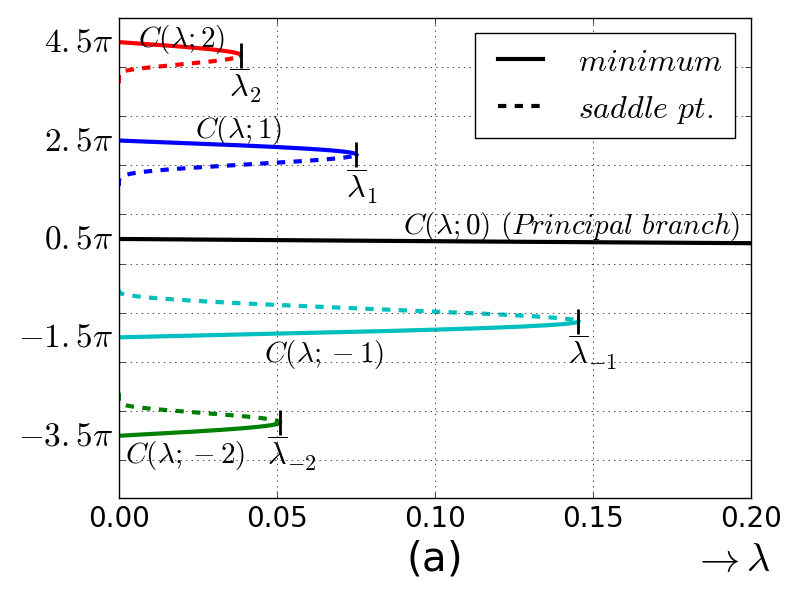
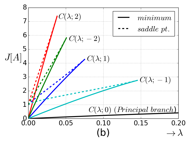
Figure 1: (a) Critical points in Example 1 (the $(2,1)$ entry of the solution matrix $C(\lambda;n)$ is depicted for $n=0,\pm 1,\pm 2$); (b) The cost $J[A]$ for these solutions.

The software package PyDSTool Clewley et al. (2007) is used to numerically continue the solution $C(\lambda;n)$ as a function of the parameter $\lambda$. Figure 1(a) depicts the solutions branches in terms of the $(2,1)$ entry of the matrix $C(\lambda;n)$ for $n=0,\pm 1,\pm 2$. The following observations are made concerning these solutions:

• For each fixed $n\neq 0$, there exist a range $(0,\bar{\lambda}_{n})$ for which there exist two solutions, a local minimum and a saddle point. At the limit (turning) point $\lambda=\bar{\lambda}_{n}$, there is a qualitative change in the solution from a minimum to a saddle point.

• As a function of $n$, $\bar{\lambda}_{n}$ decreases monotonically as $|n|$ increases. For $\lambda>\bar{\lambda}_{-1}$, only a single solution, the principal branch $C(\lambda;0)$ was found using numerical continuation.

• Along the branch with a fixed $n\neq 0$, as $\lambda\downarrow 0$, the saddle point solution escapes to infinity. That is as $\lambda\downarrow 0$, the saddle point solution $C(\lambda;n)\to(\pi/2+(2n-1)\pi)\begin{bmatrix}-\infty&-1\\ 1&-\infty\end{bmatrix}$. The associated cost $J[A]\downarrow 1$ (The cost of global minimizer $J^{*}=0$).

• Among the numerically obtained solution branches, the principal branch $C(\lambda;0)$ has the lowest cost. Figure 1 (b) depicts the cost for the solutions depicted in Figure 1 (a).

The numerical calculations indicate that while the $[\lambda=0]$ problem has infinitely many critical points (all global minimizers), only a few of these critical points persist for any finite positive value of $\lambda$. Moreover, there exists both local (but not global) minimum as well as saddle points for this case. Among the solutions computed, the principal branch (continued from the principal logarithm $C(0;0)$) has the minimum cost.

Example 2 (Non-normal).

Numerical continuation is used to obtain solutions for non-normal $R=\begin{bmatrix}0&-1\\ 1&\mu\end{bmatrix}$, where $\mu$ is a continuation parameter and $T=1$. Figure 2(a) depicts a solution branch as a function of parameter $\mu$. The solution is initialized with the normal solution ${\sf C}(0;0)$ described in Example 1. By varying $\mu$, the solution is continued to $\mu=\pi/2$ (indicated as ${\color[rgb]{1,0,0}\diamond}$ in part (a)). This way, the solution ${\sf C}=\begin{bmatrix}0&0\\ \frac{\pi}{2}&0\end{bmatrix}$ is found for $R=\begin{bmatrix}0&-1\\ 1&\frac{\pi}{2}\end{bmatrix}$. It is easy to verify that ${\sf C}$ is a solution of the characteristic equation (18) for $\lambda=0$ and $T=1$. For this solution, the critical point of the optimal control problem

$$A_{t}=\begin{bmatrix}-\pi\sin(\pi t)&\pi\cos(\pi t)-\pi\\ \pi\cos(\pi t)+\pi&\pi\sin(\pi t)\end{bmatrix}$$

is non-constant. It is noted that the principal logarithm $\log(R)=\begin{bmatrix}-\gamma\tan\gamma&-\gamma\sec\gamma\\ \gamma\sec\gamma&\gamma\tan\gamma\end{bmatrix}$, where $\gamma=\sin^{-1}\left(\dfrac{\pi}{4}\right)$. The regularization cost for the non-constant solution $A_{t}$ is strictly smaller than the constant $\frac{1}{T}\log(R)$ solution:

$$\int_{0}^{1}\mbox{tr}(A_{t}A_{t}^{\top})\,\mathrm{d}t=\int_{0}^{1}\mbox{tr}({\sf C}{\sf C}^{\top})\,\mathrm{d}t =\frac{\pi^{2}}{4}<3.76=\int_{0}^{1}\mbox{tr}(\log(R)\log(R)^{\top})\,\mathrm{d}t$$

Next, the parameter $\mu=\frac{\pi}{2}$ is fixed, and the solution continued in the parameter $\lambda$. Figure 2(b) depicts the cost $J[A]$ for the resulting solution branch of critical points (minimum). The cost with the constant $\frac{1}{T}\log(R)$ is also depicted. It is noted that the latter is not a critical point of the optimal control problem for any positive value of $\lambda$.

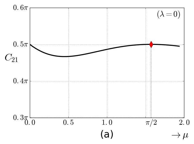
Figure 2: (a) Numerical continuation of the solution in Example 2; (b) The cost $J[A]$ for the critical point (minimum) and the constant $\frac{1}{T}\log(R)$ solution.

4 Conclusion

In this paper, the non convex optimization problem of learning the weights of a linear network with a regularized model of mean-squared loss function was introduced and studied. The regularized model (4) is likely to reveal features (both good and bad) which are robust and as such likely to be seen in an implementation of the backprop algorithm. For example, it was shown that the regularization serves to constrain the number and type of critical points (see Remark 2). Also, saddle points can appear when none exist for the $[\lambda=0]$ problem (see Example 1). The focus of the continuing research concerns the generalization property and the stability of the critical points.

5 Appendix

Notation: For all $B\in M_{d}(\mathbb{R})$, the Frobenius norm is denoted as $\|B\|$ given by $\|B\|:=\sqrt{\mbox{tr}(BB^{\top})}$.

5.1 Scalar case

The scalar case is proved using elementary means and is useful to both introduce the characteristic equation as well as highlight the difference between the $[\lambda=0]$ and the $[\lambda=0^{+}]$ problems.

Theorem 3.

Consider the terminal cost optimal control problem (4) for the scalar ($d=1$) case with $R>0$ and $\Sigma_{0}={\sf E}[X_{0}^{2}]>0$ given. If $A_{t}$ is a minimizer then

$$A_{t}\equiv{\sf C},\quad X_{t}=e^{t{\sf C}}X_{0}$$ (20)

where the constant ${\sf C}$ is a solution of the characteristic equation

$$\lambda{\sf C}=e^{T{\sf C}}(R-e^{T{\sf C}})\Sigma_{0}$$ (21)

Conversely a solution ${\sf C}$ of the characteristic equation (21) defines a critical point (20) of the optimal control problem (4).

The following is a complete characterization of the solutions ${\sf C}$ of the characteristic equation (21) as a function of parameters $(\lambda,R,\Sigma_{0},T)\in\mathbb{R}^{+}\times\mathbb{R}^{+}\times\mathbb{R}^{+}\times\mathbb{R}^{+}$:

• For $\lambda\in[0,2e^{3}\Sigma_{0}T]$ there exists a unique solution. The associated solution obtained using (20) is a minimizer.

• In the asymptotic limit as $\lambda\downarrow 0$, the minimizer is given by an asymptotic expansion

  $${\sf C}=\frac{1}{T}\log(R)-\lambda\frac{\log(R)}{T^{2}R^{2}\Sigma_{0}}+O(\lambda^{2})$$ (22)

  The unique solution for the $\lambda=0^{+}$ problem, obtained by retaining the first order term, is given by ${\sf C}=\frac{1}{T}\log(R)$.

• For $\lambda>2e^{3}\Sigma_{0}T$, there exists an interval such that for $R\in[R_{1}(\lambda),R_{2}(\lambda)]$ there are exactly 3 solutions of the characteristic equation. For $R>R_{2}(\lambda)$ or $R<R_{1}(\lambda)$ there exists exactly one solution.

Proof.

In the scalar case, the state is given by the explicit formula $X_{t}=e^{\int_{0}^{t}A_{s}\,\mathrm{d}s}X_{0}$. Therefore, the objective function

$${\sf J}[A]=\lambda\int_{0}^{T}A_{t}^{2}\,\mathrm{d}t+(e^{\int_{0}^{T}A_{t}\,\mathrm{d}t}-R)^{2}\Sigma_{0}$$

Using the Jensen’s inequality

$${\sf J}[A] \geq\frac{\lambda}{T}(\int_{0}^{T}A_{t}\,\mathrm{d}t)^{2}+(e^{\int_{0}^{T}A_{t}\,\mathrm{d}t}-R)^{2}\Sigma$$

with an equality iff $A_{t}\equiv{\sf C}$, a constant. Therefore

$$\min_{A\in L^{2}}~{}J(A)=\min_{{\sf C}\in\mathbb{R}}~{}\lambda T{\sf C}^{2}+(e^{T{\sf C}}-R)^{2}\Sigma$$

The characteristic equation is the first order optimality condition of the right hand side.

• Denote $\tilde{\lambda}=\frac{\lambda}{T\Sigma}$ and $\tilde{\sf C}=T{\sf C}$ to write the characteristic equation as

  $$f(\tilde{\sf C},\tilde{\lambda}):=\tilde{\lambda}\tilde{\sf C}e^{-\tilde{\sf C}}+e^{\tilde{\sf C}}=R$$ (23)

  For $\tilde{\lambda}=0$, the solution $\tilde{\sf C}=\log(R)$. For $\lambda>0$, $f$ is onto (since $f$ is continuous and $\lim_{\tilde{\sf C}\to\pm\infty}f(\tilde{\sf C})=\pm\infty$). Therefore, there exists at least one solution for each given $R$. Since $f^{\prime}(\tilde{\sf C})=\lambda e^{-\tilde{\sf C}}(1-\tilde{\sf C})+e^{\tilde{\sf C}}>0$ for $\tilde{\sf C}\leq 1$, $f$ is monotone on $(-\infty,1]$. Also $f^{\prime}(\tilde{\sf C})=0\Leftrightarrow\lambda=\frac{e^{2\tilde{\sf C}}}{\tilde{\sf C}-1}$ and $\frac{e^{2\tilde{\sf C}}}{\tilde{\sf C}-1}$ is a unimodal convex function for $\tilde{\sf C}>1$ with minimum $2e^{3}$ at $\tilde{\sf C}=3/2$. Therefore for $\tilde{\lambda}\leq 2e^{3}$, $f$ is monotone over entire $\mathbb{R}$. This implies that the solution to $f(\tilde{\sf C})=R$ is unique for $\tilde{\lambda}\leq 2e^{3}$.

• At $\tilde{\lambda}=0$, $\tilde{\sf C}=\log(R)$. Also $f^{\prime}(\log(R),0)=R\neq 0$. So by the implicit function theorem there exists a unique solution $\tilde{\lambda}\to\tilde{\sf C}(\tilde{\lambda})$ in a neighborhood of $0$. The asymptotic formula (22) for the solution is obtained by substituting regular perturbation expansion $\tilde{\sf C}=\tilde{\sf C}_{0}+\lambda\tilde{\sf C}_{1}+O(\lambda^{2})$ into (23).

  $$f(\tilde{\sf C})=\lambda\tilde{\sf C}_{0}e^{-\tilde{\sf C}_{0}}+e^{\tilde{\sf C}_{0}}(1+\lambda\tilde{\sf C}_{1})+O(\lambda^{2})=R$$

  Collecting the zeroth and the first order terms, one obtains $\tilde{\sf C}_{0}=\log(R)$ and $\tilde{\sf C}_{1}=-\frac{\log(R)}{R^{2}}$.

• If $\tilde{\lambda}>2e^{3}$, $f^{\prime}(\tilde{\sf C})=0$ has two solutions, $\tilde{\sf C}_{1}\in(3/2,\infty)$ and $\tilde{\sf C}_{2}\in(1,3/2)$. Therefore for $R\in[f(\tilde{\sf C}_{1}),f(\tilde{\sf C}_{2})]$, $f(\tilde{\sf C})=R$ has three solutions.

∎

5.2 Proof of the Proposition 1 (Hamiltonian formulation)

Let $A_{t}$ be the minimizer of (4). Define $X_{t}$ and $Y_{t}$ as the solutions of the Hamilton’s equations (7)-(8). We show $A_{t}$ satisfies (9) as follows: For $s\in[0,T]$ and $B\in M_{d}(\mathbb{R})$ consider a (needle) variation of the form:

$$A^{(\epsilon)}_{t}=\begin{cases}B\quad&t\in[s-\epsilon,s]\\ A_{t}\quad&t\notin[s-\epsilon,s]\end{cases}$$

Let $X_{t}^{(\epsilon)}$ denote the solution to the Hamitonian equation-(7) with $A_{t}^{(\epsilon)}$. It is given by:

$$X^{(\epsilon)}_{t}=X_{t}+\epsilon\eta_{t}+O(\epsilon^{2})$$

where for $t<s$, $\eta_{t}=0$ and for $t>s$, $\eta_{t}$ is the solution of

$$\frac{\,\mathrm{d}\eta_{t}}{\,\mathrm{d}t}=A_{t}\eta_{t},\quad\text{with i.c}\quad\eta_{s}=(B-A_{s})X_{s}$$

The perturbed cost is

$${\sf J}[A^{(\epsilon)}]={\sf J}[A] +\epsilon\lambda(\text{Tr}(B^{\top}B)-\text{Tr}(A_{s}^{\top}A_{s}))+2\epsilon{\sf E}[(X_{T}-Z)^{\top}\eta_{T}]+O(\epsilon^{2})$$

Since $A_{t}$ is a minimizer

$$\frac{\lambda}{2}(\text{Tr}(B^{\top}B)-\text{Tr}(A_{s}^{\top}A_{s}))+{\sf E}[(X_{T}-Z)^{\top}\eta_{T}]\geq 0$$

The next step is to obtain $(X_{T}-Z)^{\top}\eta_{T}$ in terms of $Y_{t}$. By construction $\frac{\,\mathrm{d}}{\,\mathrm{d}t}Y_{t}^{\top}\eta_{t}=0$. Therefore,

$$(Z-X_{T})^{\top}\eta_{T}=Y_{T}^{\top}\eta_{T}=Y_{s}^{\top}\eta_{s}=Y_{s}^{\top}(B-A_{s})X_{s}$$

and hence

$$\frac{\lambda}{2}(\text{Tr}(B^{\top}B)-\text{Tr}(A_{s}^{\top}A_{s}))-{\sf E}[Y_{s}^{\top}(B-A_{s})X_{s}]\geq 0,$$

On collecting the terms, one obtains

$${\sf E}[H(X_{s},Y_{s},A_{s})]\geq{\sf E}[H(X_{s},Y_{s},B)]\quad\forall B\in M_{d}(\mathbb{R})$$

Since $s\in[0,T]$ is arbitrary, the result follows.

5.3 First order variation of ${\sf J}$

Let $X_{t}$ and $Y_{t}$ be the solutions to the Hamilton’s equations-(7)-(8) with weight matrix $A_{t}$. Define $A^{(\epsilon)}_{t}=A_{t}+\epsilon V_{t}$. Let $X^{(\epsilon)}_{t}$ and $Y^{(\epsilon)}_{t}$ be the solutions to the Hamilton’s equations with weight matrix $A^{(\epsilon)}_{t}$. In the limit as $\epsilon\to 0$, $X_{t}^{(\epsilon)}$ is given by the asymptotic formula $X_{t}^{(\epsilon)}=X_{t}+\epsilon\eta_{t}+O(\epsilon^{2})$ where

$$\frac{\,\mathrm{d}\eta_{t}}{\,\mathrm{d}t}=A_{t}\eta_{t}+V_{t}X_{t},\quad\eta_{0}=0$$

In terms of $\eta_{t}$, the objective function

$${\sf J}[A^{(\epsilon)}]={\sf J}[A]+\epsilon\left(\lambda\int_{0}^{T}\mbox{tr}(A_{t}^{\top}V_{t})+{\sf E}[{(X_{T}-Z)^{\top}\eta_{T}}]\right)+O(\epsilon^{2})$$

Use the definition of $Y_{t}$ to express $(X_{T}-Z)^{\top}\eta_{T}$ as

$$(Z-X_{T})^{\top}\eta_{T}=Y_{T}^{\top}\eta_{T}=\int_{0}^{T}\frac{\,\mathrm{d}}{\,\mathrm{d}t}(Y_{t}^{\top}\eta_{t})\,\mathrm{d}t=\int_{0}^{T}(-Y_{t}^{\top}A_{t}\eta_{t}+Y_{t}^{\top}A_{t}\eta_{t}+Y_{t}^{\top}V_{t}X_{t})\,\mathrm{d}t=\int_{0}^{T}Y_{t}^{\top}V_{t}X_{t}\,\mathrm{d}t$$

Therefore,

$${\sf J}[A^{(\epsilon)}] ={\sf J}[A]+\epsilon\int_{0}^{T}{\sf E}{\left[\mbox{tr}\left((\lambda A_{t}^{\top}-X_{t}Y_{t}^{\top})V_{t}\right)\right]}\,\mathrm{d}t+O(\epsilon^{2})$$

On the other hand $\frac{\partial H}{\partial B}(x,y,B)=\lambda B+yx^{\top}$. Therefore

$${\sf J}[A^{(\epsilon)}]-{\sf J}[A]=\epsilon\int_{0}^{T}\mbox{tr}\left({\sf E}\left[\frac{\partial H}{\partial B}(X_{t},Y_{t},A_{t})\right]^{\top}V_{t}\right)\,\mathrm{d}t+O(\epsilon^{2})$$

which gives the result $\nabla{\sf J}[A]=-{\sf E}[\frac{\partial H}{\partial B}(X_{t},Y_{t},A_{t})]$.

5.4 Proof of the Theorem 14

For the [$\lambda=0$] problem, the gradient $\nabla{\sf J}[A]$ is (by (10))

$$\nabla{\sf J}[A]=-{\sf E}[Y_{t}X_{t}^{\top}]$$

where $X_{t}$ and $Y_{t}$ solve the Hamilton’s equations-(7)-(8). Define the state transition matrix $\phi(t,t_{0})$ of the differential equation $\frac{\,\mathrm{d}X_{t}}{\,\mathrm{d}t}=A_{t}X_{t}$ according to:

$$\frac{\,\mathrm{d}\phi({t,t_{0}})}{\,\mathrm{d}t}=A_{t}\phi({t,t_{0}}),\quad\phi({t_{0},t_{0}})=I$$

In terms of the transition matrix,

$$X_{t} =\phi(t,0)X_{0},\quad Y_{t}=\phi({T,t})^{\top}(Z-X_{T})$$

Therefore

$$\nabla{\sf J}[A]=-\phi({T,t})^{\top}(R-\phi({T,0}))\Sigma\phi({t,0})^{\top}=:\psi_{t}$$

Since $\phi({t,t_{0}})$ is invertible

$$\nabla{\sf J}[A]=0\quad\Leftrightarrow\quad R=\phi({T,0})\quad\Leftrightarrow\quad{\sf J}[A]=J^{*}={\sf E}[|W|^{2}]$$

For each fixed $t\in[0,T]$

$$\|\psi_{t}\|^{2} =\|\phi({T,t})^{\top}(R-\phi({T,0}))\Sigma\phi({t,0})^{\top}\|^{2}$$

$$\geq\lambda_{\text{min}}(\phi({T,t})^{\top}\phi({T,t}))\lambda_{\text{min}}(\phi({t,0})^{\top}\phi({t,0}))\|(R-\phi({T,0}))\Sigma\|^{2}$$

$$\geq\lambda_{\text{min}}(\phi({T,t})^{\top}\phi({T,t}))\lambda_{\text{min}}(\phi({t,0})^{\top}\phi({t,0}))\lambda_{\text{min}}(\Sigma)\mbox{tr}((R-\phi({T,0}))^{\top}(R-\phi({T,0}))\Sigma)$$

$$\geq e^{-2\int_{0}^{T}|\|A_{t}\|\,\mathrm{d}t}\lambda_{\text{min}}(\Sigma)({\sf J}[A]-{\sf J}^{*})$$

where we used Lemma 5.1 (see below) in the last step. Integrating the inequality on $[0,T]$ yields the result.

Lemma 5.1.

Let $\phi({t,t_{0}})$ be the state transition matrix defined according to $\frac{\,\mathrm{d}}{\,\mathrm{d}t}\phi({t,t_{0}})=A_{t}\phi({t,t_{0}})$ with $\phi({t_{0},t_{0}})=I$. Then,

$$e^{-2\int_{0}^{t}\|A_{t}\|\,\mathrm{d}t}\leq\lambda_{\text{min}}(\phi({t,0})^{\top}\phi({t,0}))\leq\lambda_{\text{max}}(\phi({t,0})^{\top}\phi({t,0}))\leq e^{2\int_{0}^{t}\|A_{t}\|\,\mathrm{d}t}$$

Proof.

Observe that

$$\lambda_{\text{max}}(\phi({t,0})^{\top}\phi({t,0})) =\max_{x\neq 0}\frac{x^{\top}\phi_{t,0}^{\top}\phi_{t,0}x}{x^{\top}x}=\max_{x_{0}\neq 0}\frac{x_{t}^{\top}x_{t}}{x_{0}^{\top}x_{0}}$$

Now,

$$\frac{\,\mathrm{d}}{\,\mathrm{d}t}|x_{t}|^{2}=x_{t}^{\top}(A_{t}+A_{t}^{\top})x_{t}\leq\lambda_{\text{max}}(A_{t}+A_{t}^{\top})|x_{t}|^{2}\leq 2\|A_{t}\||x_{t}|^{2}$$

where the last inequality follows because $2\|A_{t}\|=\|A_{t}+A_{t}^{\top}\|\geq\lambda_{\text{max}}(A_{t}+A_{t}^{\top})$. Therefore, $|x_{t}|^{2}\leq e^{2\int_{0}^{t}\|A_{t}\|\,\mathrm{d}t}|x_{0}|^{2}$ which gives the upper bound. The calculation for the lower bound is similar. ∎

5.5 Convergence of the learning algorithm

Proposition 3.

Consider the stochastic gradient descent learning algorithm (11) with $\lambda=0$. Suppose $\exists\alpha>0$ such that ${\sf E}[X_{0}X_{0}^{T}QX_{0}X_{0}^{T}]\leq\alpha\Sigma_{0}Q\Sigma_{0}$ for all symmetric matrices $Q$, and $\|A^{(k)}\|_{L^{2}}\leq M$ for all $k\in\mathbb{N}$. Then there exists a positive constant $\beta>0$ such that ${\sf J}$ is a $\beta$-smooth function. And for sufficiently small constant stepsize $\eta_{k}=\eta\leq\frac{1}{\alpha\beta}$,

$${\sf J}[A^{(k)}]-{\sf J}^{*}\leq(1-\frac{\eta}{2})^{k}({\sf J}[A^{(0)}]-{\sf J}^{*})+\eta\beta e^{2M\sqrt{T}}{\sf E}[|X_{0}|^{2}|\xi|^{2}],$$

for all $k\in\mathbb{N}$ where ${\sf J}^{*}:=\min_{A}{\sf J}[A]=E[|\xi|^{2}]$.

Proof.

The proof is based on Theorem 4.8 in Bottou et al. [2016] where it is shown that SGD converges to a local minimum. To apply the theorem we show

$${\sf E}\left[Y_{t}^{(k)}{X_{t}^{(k)}}^{\top}\right] =\nabla{\sf J}[A^{(k)}]$$

because $X^{(k)}_{0}$ is a random sample of $X_{0}$ and $\nabla{\sf J}[A^{(K)}]$ is given by the formula (10) for $\lambda=0$. Next

$${\sf E}\left[\left\|Y_{t}^{(k)}{X_{t}^{(k)}}^{\top}\right\|^{2}\right] ={\sf E}\left[\|\phi({T,t})^{\top}(Z-X^{i}_{T}){X_{0}^{i}}^{\top}\phi({t,0})^{\top}\|^{2}\right]$$

$$={\sf E}\left[\|\phi({T,t})^{\top}(R-\phi({T,0}))X_{0}X_{0}^{\top}\phi({t,0})^{\top}\|^{2}\right]+{\sf E}\left[\|\phi({T,t})^{\top}WX_{0}^{\top}\phi({t,0})^{\top}\|^{2}\right]$$

$$\leq\alpha\|\phi({T,t})^{\top}(R-\phi({T,0}))\Sigma\phi({t,0})^{\top}\|^{2}+e^{2\int_{0}^{T}\|A_{t}\|\,\mathrm{d}t}{\sf E}[|W|^{2}]{\sf E}[|X_{0}|^{2}]$$

where the assumption ${\sf E}[X_{0}X_{0}^{\top}\phi({t,0})^{\top}\phi({t,0})X_{0}X_{0}^{\top}]\leq\alpha\Sigma\phi({t,0})^{\top}\phi({t,0})\Sigma$ and Lemma 5.1 is used.

The fact that ${\sf J}$ is $\beta$-smooth is true since all the functions involved are smooth and it is assumed $A$ is bounded. Applying Theorem 4.8 in Bottou et al. [2016], SGD algorithm converges to a local minimum. The geometric convergence to the global minimum follows from Theorem 14 where it is shown that local minimum are global minimum for $\lambda=0$ and using the inequality (14). ∎

5.6 Proof of Proposition 2

Suppose $(X_{t},Y_{t},A_{t})$ is a solution of the Hamilton’s equations(7)-(9). Then by differentiating $A_{t}$ with respect to $t$, one obtains

$$\frac{\,\mathrm{d}A_{t}}{\,\mathrm{d}t}=-A_{t}^{\top}A_{t}+A_{t}A_{t}^{\top}$$

On expressing $A_{t}=S_{t}+\Omega_{t}$ as the sum of its symmetric component $S_{t}=\frac{1}{2}(A_{t}+A_{t}^{\top})$ and the skew-symmetric component $\Omega_{t}=\frac{1}{2}(A_{t}-A_{t}^{\top})$, one obtains

$$\frac{\,\mathrm{d}S_{t}}{\,\mathrm{d}t} =2\Omega_{t}S_{t}-2S_{t}\Omega_{t},\quad\frac{\,\mathrm{d}\Omega_{t}}{\,\mathrm{d}t}=0$$

whose solution is given by

$$S_{t} =e^{2t\Omega}S_{0}e^{-2t\Omega},\quad\Omega_{t}=\Omega_{0}$$

This gives (17).

Using the formula (17) for $A_{t}$, the Hamilton’s equation for $X_{t}$ is

$$\frac{\,\mathrm{d}X_{t}}{\,\mathrm{d}t}=e^{2t\Omega}Se^{-2t\Omega}X_{t}+\Omega X_{t}$$

whose solution is given by (15).

The optimal costate trajectory is obtained similarly. The Hamilton’s equation for the costate is:

$$\frac{\,\mathrm{d}Y_{t}}{\,\mathrm{d}t}=-e^{2t\Omega}Se^{-2t\Omega}Y_{t}+\Omega Y_{t},\quad Y_{T}=Z-X_{T}$$

whose solution is given by (16).

The characteristic equation (18) is obtained by using the formula $A_{t}=\frac{1}{\lambda}{\sf E}[Y_{t}X_{t}^{\prime}]$:

$$\lambda e^{2t\Omega}{\sf C}e^{-2t\Omega}=e^{2t\Omega}e^{-t{\sf C}}e^{T{\sf C}}e^{-2T\Omega}{\sf E}[(Z-X_{T})X_{0}^{\top}]e^{t{\sf C}}e^{-2t\Omega}$$

upon multiplying both sides from left by $e^{t{\sf C}}e^{-2t\Omega}$ and from right by $e^{2t\Omega}e^{-t{\sf C}}$.

Optimal cost: Optimal cost is obtained by inserting $A_{t}=e^{2t\Omega}{\sf C}e^{-2t\Omega}$ into the cost function where the following identities are used:

$$\mbox{tr}(A_{t}A_{t}^{\top}) =\mbox{tr}({\sf C}{\sf C}^{\top})$$

$${\sf E}[|X_{T}-Z|^{2}] ={\sf E}[|W|^{2}]+{\sf E}[|FX_{0}-RX_{0}|^{2}]$$

Constant $\Leftrightarrow$ normal: Suppose $A_{t}=C$ a constant. Then $\frac{\,\mathrm{d}A_{t}}{\,\mathrm{d}t}=-A_{t}^{\top}A_{t}+A_{t}A_{t}^{\top}=0$, and hence $A_{t}=C$ is a normal matrix. Conversely, assuming $A_{t}$ is a normal matrix implies $\frac{\,\mathrm{d}A_{t}}{\,\mathrm{d}t}=0$ and hence $A_{t}=C$ a constant.

Normal solution: If ${\sf C}$ is normal, then ${\sf C}$ and $\Omega$ commute, therefore $F=e^{T{\sf C}}$. Hence the characteristic simplifies to

$$\lambda{\sf C}=e^{{\sf C}^{\top}}(R-e^{{\sf C}})\Sigma$$

and equivalently

$$\lambda{\sf C}e^{-{\sf C}^{\top}}\Sigma^{-1}+e^{{\sf C}}=R$$

Therefore, if ${\sf C}$ and $\Sigma$ commute (always true when $\Sigma=I$), $R$ is a normal matrix. We have proved

$$A_{t}\equiv{\sf C}~{}~{}\Longleftrightarrow~{}~{}{\sf C}~{}~{}\text{is normal}~{}~{}\overset{(\Sigma=I)}{\Longrightarrow}~{}~{}R~{}~{}\text{is normal}$$

Therefore a non-normal $R$ implies the minimizer $A_{t}$ is not constant for $\Sigma=I$.

5.7 Proof of Theorem 2

1. If ${\sf C}$ is normal, then $e^{T({\sf C}-{\sf C}^{\top})}e^{T{\sf C}}=e^{T{\sf C}}$. Hence for $\lambda=0$ problem the characteristic equation becomes $e^{T{\sf C}}=R$ whose solution is ${\sf C}=\frac{1}{T}\log(R)$, interpreted as multi-valued matrix logarithm function (see Higham [2014]).

2. For $\lambda>0$ and $\Sigma=I$ the characteristic equation is:

   $$\lambda{\sf C}e^{-{\sf C}^{\top}}+e^{{\sf C}}=R$$

   Since ${\sf C}$ is normal, $R$ must be normal and moreover there exists a unitary (complex) matrix $U$ such that $U^{*}RU=D$ where $D=\text{diag}(r_{1},\ldots,r_{d})$ with $r_{n}\in\mathbb{C}$. Let $\mu_{n}\in\mathbb{C}$ be solution to the equation

   $$\lambda\mu_{n}e^{-\mu_{n}^{*}}+e^{\mu_{n}}=r_{n}$$ (24)

   for $n=1,\ldots,d$. Then ${\sf C}=UGU^{*}$ where $G=\text{diag}(\mu_{1},\ldots,\mu_{d})$ is the normal solution to the characteristic equation since

   $$\lambda Ge^{-G^{*}}+e^{G}=D\quad\Rightarrow\quad\lambda UGe^{-G^{*}}U^{*}+Ue^{G}U^{*}=UDU^{*}\quad\Rightarrow\quad\lambda{\sf C}e^{{\sf C}^{\top}}+e^{\sf C}=R$$

   It thus suffices to analyze solutions to the complex equation (24). Denoting $\mu_{n}=x+iy$ and $r_{n}=e^{a+i\theta}$ the complex equation (24) is written as two real equations:

   $$f_{1}(x,y;\lambda):=\lambda xe^{-x}\cos(y)-\lambda ye^{-x}\sin(y)+e^{x}\cos(y) =e^{a}\cos(\theta)$$

   $$f_{2}(x,y;\lambda):=\lambda xe^{-x}\sin(y)+\lambda ye^{-x}\cos(y)+e^{x}\sin(y) =e^{a}\sin(\theta)$$

   At $\lambda=0$, there are countability many solutions given by $x_{0}=a$ and $y_{0}=\theta+m2\pi$ for $m\in\mathbb{Z}$. The Jacobian

   $$\mathsf{D}f(x_{0},y_{0};0)=\begin{bmatrix}\frac{\partial f_{1}}{\partial x}(x_{0},y_{0},0)&\frac{\partial f_{1}}{\partial y}(x_{0},y_{0},0)\\ \frac{\partial f_{2}}{\partial x}(x_{0},y_{0},0)&\frac{\partial f_{2}}{\partial y}(x_{0},y_{0},0)\end{bmatrix}=\begin{bmatrix}e^{x_{0}}\cos(y_{0})&-e^{x_{0}}\sin(y_{0})\\ e^{x_{0}}\sin(y_{0})&e^{x_{0}}\cos(y_{0})\end{bmatrix}$$

   is nonsingular since $\text{det}(\mathsf{D}f)=e^{2x_{0}}=e^{2a}>0$. Therefore, using the implicit function theorem, there exists a neighborhood $\cal{N}$ of $\lambda=0$ and a function $\lambda\in\mathcal{N}\to(x(\lambda),y(\lambda))\in\mathbb{R}^{2}$ such that $f(x(\lambda),y(\lambda);\lambda)=0$. The asymptotic formula for $x(\lambda)$ and $y(\lambda)$ are obtained upon using a regular perturbation expansion $x=x_{0}+\lambda x_{1}+O(\lambda^{2})$ and $y=y_{0}+\lambda y_{1}+O(\lambda^{2})$. Then

   $$\begin{bmatrix}x_{1}\\ y_{1}\end{bmatrix} =-[\mathsf{D}f(x_{0},y_{0};0)]^{-1}\frac{\partial f}{\partial\lambda}(x_{0},y_{0};0)$$

   $$=-e^{-x_{0}}\begin{bmatrix}\cos(y)&\sin(y_{0})\\ -\sin(y)&\cos(y_{0})\end{bmatrix}\begin{bmatrix}x_{0}e^{-x_{0}}\cos(y_{0})-y_{0}e^{-x_{0}}\sin(y_{0})\\ x_{0}e^{-x_{0}}\sin(y_{0})+y_{0}e^{-x_{0}}\cos(y_{0})\end{bmatrix}$$

   $$=-e^{-2x_{0}}\begin{bmatrix}x_{0}\\ y_{0}\end{bmatrix}$$

   Therefore

   $$\mu=\log(r)-\lambda\frac{\log(r)}{|r|^{2}}+O(\lambda^{2})$$

   which gives the asymptotic formula

   $${\sf C}=\log(R)-\lambda(RR^{*})^{-1}\log(R)+O(\lambda^{2})$$

References

- Baldi and Hornik [1989] P. F. Baldi and K. Hornik. Neural networks and principal component analysis: Learning from examples without local minima. Neural networks, 2(1):53–58, 1989.
- Baldi and Hornik [1995] P. F. Baldi and K. Hornik. Learning in linear neural networks: A survey. IEEE Transactions on neural networks, 6(4):837–858, 1995.
- Bottou et al. [2016] L. Bottou, F. E. Curtis, and J. Nocedal. Optimization methods for large-scale machine learning. arXiv:1606.04838, June 2016.
- Choromanska et al. [2015a] A. Choromanska, M. Henaff, M. Mathieu, G. B. Arous, and Y. LeCun. The loss surfaces of multilayer networks. In AISTATS, 2015a.
- Choromanska et al. [2015b] A. Choromanska, Y. LeCun, and G. B. Arous. Open problem: The landscape of the loss surfaces of multilayer networks. In COLT, pages 1756–1760, 2015b.
- Clewley et al. [2007] R. Clewley, W. E. Sherwood, M. D. LaMar, and J. Guckenheimer. Pydstool, a software environment for dynamical systems modeling, 2007. URL http://pydstool.sourceforge.net.
- Culver [1966] W. J. Culver. On the existence and uniqueness of the real logarithm of a matrix. Proceedings of the American Mathematical Society, 17(5):1146–1151, 1966.
- Dauphin et al. [2014] Y. N. Dauphin, R. Pascanu, C. Gulcehre, K. Cho, S. Ganguli, and Y. Bengio. Identifying and attacking the saddle point problem in high-dimensional non-convex optimization. In Advances in neural information processing systems, pages 2933–2941, 2014.
- Farotimi et al. [1991] O. Farotimi, A. Dembo, and T. Kailath. A general weight matrix formulation using optimal control. IEEE Transactions on neural networks, 2(3):378–394, 1991.
- Ge et al. [2015] R. Ge, F. Huang, C. Jin, and Y. Yuan. Escaping From Saddle Points — Online Stochastic Gradient for Tensor Decomposition. arXiv:1503.02101, March 2015.
- Hardt and Ma [2016] M. Hardt and T. Ma. Identity matters in deep learning. arXiv:1611.04231, November 2016.
- Higham [2014] N. J. Higham. Functions of matrices. CRC Press, 2014.
- Kawaguchi [2016] K. Kawaguchi. Deep learning without poor local minima. In Advances In Neural Information Processing Systems, pages 586–594, 2016.
- LeCun et al. [1988] Y. LeCun, D. Touresky, G. Hinton, and T. Sejnowski. A theoretical framework for back-propagation. In The Connectionist Models Summer School, volume 1, pages 21–28, 1988.
- Lee et al. [2016] J. D. Lee, M. Simchowitz, M. I. Jordan, and B. Recht. Gradient Descent Converges to Minimizers. arXiv:1602.04915, February 2016.
- Saxe et al. [2013] A. M. Saxe, J. L. McClelland, and S. Ganguli. Exact solutions to the nonlinear dynamics of learning in deep linear neural networks. arXiv:1312.6120, December 2013.
- Soudry and Carmon [2016] D. Soudry and Y. Carmon. No bad local minima: Data independent training error guarantees for multilayer neural networks. arXiv:1605.08361, May 2016.