The CARMA 3 mm Survey of the Inner $0.7^{\circ}\times 0.4^{\circ}$ of the Central Molecular Zone

Abstract

The Central Molecular Zone (CMZ) of the Galactic Center has to date only been fully mapped at mm wavelengths with singledish telescopes, with resolution about 30″ (1.2 pc). Using CARMA, we mapped the innermost 0.25 square degrees of the CMZ over the region between –0$.\kern-2.5pt^{{}^{\circ}}$2$\leq l\leq$0$.\kern-2.5pt^{{}^{\circ}}$5 and –0$.\kern-2.5pt^{{}^{\circ}}$2$\leq b\leq$0$.\kern-2.5pt^{{}^{\circ}}$2 (90$\times$50 pc) with spatial and spectral resolution of $\sim 10\arcsec$ (0.4 pc) and $\sim 2.5~{}{\,{\rm km~{}s^{-1}}}$, respectively. We provide a catalog of 3 mm continuum sources as well as spectral line images of SiO(J=2-1), HCO⁺(J=1-0), HCN(J=1-0), N₂H⁺(J=1-0), and CS(J=2-1), with velocity coverage V_LSR= –200 to 200 ${\rm km~{}s^{-1}}$. To recover the large scale structure resolved out by the interferometer, the continuum-subtracted spectral line images were combined with data from the Mopra 22-m telescope survey, thus providing maps containing all spatial frequencies down to the resolution limit. We find that integrated intensity ratio of I(HCN)/I(HCO⁺) is anti-correlated with the intensity of the 6.4 keV Fe K$\alpha$, which is excited either by high energy photons or low energy cosmic rays, and the gas velocity dispersion as traced by HCO⁺ is correlated with Fe K$\alpha$ intensity. The intensity ratio and velocity dispersion patterns are consistent with variation expected from the interaction of low energy cosmic rays with molecular gas.

1 Introduction

The inner few hundred pc of the Galactic Center differs from the rest of the Galaxy in its ISM properties. The central molecular zone (CMZ) is occupied by an impressive collection of massive molecular clouds which are characterized by a rich chemistry, broad linewidths, elevated temperatures and high density compared to those in the disk of the Galaxy. There are several observations suggesting that the ISM in this region is also characterized by strong nonthermal emission compared to the rest of the Galaxy. First, radio continuum observations have uncovered a population of filamentary structures within the two degrees of the Galactic Center (e.g., Yusef-Zadeh et al., 1984; Nord et al., 2004). Their transverse dimensions are of the order of 1 pc and their length is of the order of tens of parsecs. Most of these filaments run perpendicular to the Galactic plane. Their strongly linear polarized emission and their radio spectral index confirm that the filaments are produced by synchrotron emission from relativistic electrons in a highly organized linear magnetic field. In addition, low frequency radio observations at 327 and 74 MHz emission suggest that the Galactic Center hosts a population of low energy relativistic particles (Brogan et al., 2003; LaRosa et al., 2005; Yusef-Zadeh et al., 2013a). Second, X-ray and $\gamma$-ray observatons detect strong sources of 6.4 keV line, and GeV and TeV $\gamma$-ray emission (Ponti et al., 2010; HESS Collaboration et al., 2016; Archer et al., 2016). The neutral Fe 6.4 keV K$\alpha$ line emission traces neutral cold gas. One possible interpretion of high energy activity in this region is discussed in terms a bremsstrahlung emission due to the interaction of cosmic rays with molecular gas (Yusef-Zadeh et al., 2013b). Lastly, recent measurements indicate a vast amount of H${}_{3}^{+}$ (Oka et al., 2005; Goto et al., 2014; Le Petit et al., 2016) distributed in the Galactic Center region, indicative of a high rate of ionization of H₂. The inferred cosmic ray ionization rate, $\zeta\sim 10^{-15}$  s^-1  H^-1, is one to two orders of magnitude higher in the Galactic Center region than in the Galactic disk. A possible cause of the abundance of molecular gas in the Galactic Center has also been discussed in the context of cosmic rays (Coutens et al., 2017). So, a key question is whether there are other chemical signatures that would support the interaction of molecular gas with relativistic particles.

Numerous molecular line survey observations of the CMZ over the last 30 years have solely been carried out with single dish telescopes with moderate resolutions. Comprehensive surveys of the CMZ have been out recently by the Mopra telescope at 20-28 GHz (Walsh et al., 2011), 42-50 GHz (Jones et al., 2013) and 85-93 GHz (Jones et al., 2012). This latter survey fully mapped 18 molecular lines emitting from the inner 2$.\kern-2.5pt^{{}^{\circ}}$5$\times$0$.\kern-2.5pt^{{}^{\circ}}$5 ($l\times b$) and has both spatial and spectral overlap with our work.

In this paper, we present the first interferometric molecular line survey of the innermost region of the CMZ. One of the key motivations for the survey is to examine the relationship between the distribution of the molecular line and nonthermal emission in this complex region of the Galaxy. We don’t fully understand the complex gas chemistry in this region of the Galaxy but assuming that there is interaction between cosmic rays and molecular gas, the gas chemistry is expected to be driven by cosmic rays (Coutens et al., 2017). One recent example shows the evidence for thousands of collisionally excited methanol masers in the central molecular zone (Mills et al., 2015; Cotton & Yusef-Zadeh, 2016). It is not clear if these masers are produced by star formation activity or by the interaction between enhanced cosmic rays and molecular gas in the Galactic Center region.

We present molecular line maps of the survey at one transition of each of 6 molecular species. Combining these data with future multi-transition maps at high frequencies could determine the abundance of different species, and the gas density and temperature, which are needed to examine the unusual gas chemistry in this region.

We have also carried out 3 mm continuum observations of the same region observed in spectral lines. Although there is a high concentration of diffuse HII complexes distributed in the Galactic Center region, there is no published large-area, high frequency, continuum data toward this region. Previous continuum surveys of the Galactic Center have not studied the class of compact HII regions at 3 mm, which generally trace high emission measure HII regions. Our continuum measurements identify a population of ultracompact HII regions and new sites of early star formation. Again, the images presented here need multi-frequency continuum images to separate the contribution of free-free and dust emission. These measurements can then be correlated with other tracers of young massive star formation such as H₂O, methanol masers, green fuzzies, and 24 $\mu$m survey data.

2 Observations

The survey was conducted using the Combined Array for Research in Millimeter-wave Astronomy (CARMA, Bock et al., 2006). For this survey, we used two of CARMA’s science subarray modes. The first, called CARMA-15, is the 15-element array comprised of the six 10.4 m antennas and nine 6.1 m antennas. The second, CARMA-8, is the 8-element array of 3.5 m antennas. We chose CARMA-15 plus CARMA-8 over CARMA-23 (all 23 antennas cross-correlated) because the continuum bandwidth available in CARMA-23 mode was half that in CARMA-15 plus CARMA-8.

2.1 CARMA-15

During 2012-2013, we observed 527 fields with CARMA-15 in the compact D-array configuration on a full beam width hexagonal mosaic. The area covered by these fields is –0$.\kern-2.5pt^{{}^{\circ}}$2 $\leq~{}l~{}\leq~{}$0$.\kern-2.5pt^{{}^{\circ}}$5 and –0$.\kern-2.5pt^{{}^{\circ}}$2$~{}\leq~{}b~{}\leq$0$.\kern-2.5pt^{{}^{\circ}}$2. By sampling on the full beam width (60″) of the 10.4 m antennas rather than Nyquist sampling, we cover much larger area, paying a modest price in image fidelity. The CARMA-15 signals were transmitted the eight-band spectral line correlator. In the spectral correlator, the eight bands are independently positioned within the 1-9 GHz IF space, providing eight windows in each side band. Individual bands can be set to differing bandwidths between 2 MHz and 500 MHz, and with selected channel spacings. These data contain both spectral line and continuum windows. The spectral lines SiO(J=2-1), HCN(J=1-0), HCO⁺(J=1-0), N₂H⁺(J=1-0), and CS(J=2-1), were observed in four 125 MHz bandwidths with spectral resolution 781 kHz/channel. The spectral bands cover roughly V_LSR= –200 to 200 ${\rm km~{}s^{-1}}$ with velocity resolution $\Delta$V $\sim$2.5 ${\rm km~{}s^{-1}}$. The remaining four bands were used to measure continuum, each with 500 MHz bandwidth and 31.25 MHz/channel.

We added to these data another epoch of CARMA data taken in the C and D configurations of CARMA in 2009-2010. These observations obtained continuum, N₂H⁺(J=1-0), and SiO(J=2-1)  data. The 2009-2010 data are a 37-point hexagonal mosaic with total diameter $\sim 380\arcsec$, Nyquist-sampled on the 10.4 m beam and centered on Sgr A*.

2.2 CARMA-8

Using the CARMA-8 in the SL configuration, which is optimized for low declination sources, we obtained shorter uv spacing continuum data over 273 Nyquist-sampled fields covering the same area as the CARMA-15 data. The CARMA-8 signals were transmitted to the seven-band 7 GHz continuum correlator. In this correlator, seven 500 MHz bands with 31.25 MHz/channel each are independently set to broadly cover the IF space, providing seven windows in each side band.

2.3 Mapping Strategy

All 2012-2013 observations were obtained using an on-the-fly (OTF) mosaic technique in which data are continuously integrated while the antennas move to each map grid point, and integrations between map grid points are blanked and thus do not contribute to the map. This method significantly reduces observation overhead compared to the traditional “point-and-shoot” mosaic method (Storm et al., 2014). Because this technique allowed us to cover all mosaic fields at least once in each sidereal pass, it eliminates weather-related variations that could occur if different portions of the full map were covered on different days. By starting each day’s observations at a different map field, or rastering in the opposite direction, we ensured similar uv coverage in every field of the final map.

Table 1: Observation Summary

	Array		Number	Baseline (k$\lambda$)		Mapping	Flux
Date	Config.	Correlator	of Tracks	Min.	Max.	Mode	Calibrator(s)
2009/02/23 - 2010/05/10	CARMA-15 D	Spectral+Continuum	6	2.96	34.60	Mosaic	3C273,MWC349
2009/05/05 - 2010/03/28	CARMA-15 C	Spectral+Continuum	9	7.08	87.14	Mosaic	Neptune,3C273,MWC349
2010/05/18 - 2010/05/26	CARMA-15 D	Continuum	3	3.14	36.52	Mosaic	Neptune, MWC349
2012/04/18 - 2012/05/07	CARMA-15 D	Spectral+Continuum	7	3.14	36.70	OTF	Neptune, MWC349,3C273
2012/10/19 - 2013/02/02	CARMA-8 SL	Continuum	18	1.58	22.54	OTF	Neptune, Venus, MWC349,
							3C279, 2015+372
2014/12/20 - 2015/01/12	CARMA-15 D	Continuum	3	3.14	36.70	OTF	MWC349

Details of the observations are provided in Table 1. Entries in columns 1-8 respectively of Table 1 correspond to date range of observations, array configuration, correlator mode, number of sidereal tracks observed, minimum and maximum baseline separations, whether the observations were traditional mosaic or OTF, and sources used as flux calibrators. For all observations, the phase calibration source was the quasar 1733-130. The flux density of 1733-130 varied between 1.9 and 3.5 Jy over the observing period. The uncertainty in absolute flux calibration is about 10%.

The data were reduced using MIRIAD (Sault et al., 1995). After phase, amplitude, passband, and flux calibration, and flagging of bad data, visibilities were inverted onto a 1″ grid using a robust weighting value of zero (Briggs, 1995). Deconvolution was done with the MIRIAD task mossdi which uses CLEAN algorithm of Steer et al. (1984). The deconvolved maps were then restored with a fitted 2D Gaussian beam.

For spectral line images, continuum subtraction was done in the image domain by making a dirty map of the first several emission-free channels, and subtracting that image from each plane of the dirty spectral map before deconvolution. The continuum-subtracted, restored spectral line images were combined with the singledish survey from the Mopra 22-m telescope (HPBW=39″) using the MIRIAD task immerge, except for CS which was not covered by the Mopra survey (Jones et al., 2012). In this process, the Mopra antenna temperature maps were regridded to the CARMA pixel size, map center, and spectral resolution, and multiplied by 22 Jy/K (Jones et al., 2012) to convert them to Jy beam^-1. We applied flux scale correction factors to put the Mopra data after conversion to Jy on the CARMA flux scale, derived from the overlapping Fourier annulus (6.1m - 22m). Specifically the Mopra intensities were multiplied by 0.83 (SiO), 0.84 (HCN), and 0.95 (HCO⁺ and N₂H⁺). Final map parameters are given in Table 2. Columns 1-5 of Table 2 list the observed species, synthesized beam size, synthesized beam position angle, spectral resolution, and average 1$\sigma$ rms noise per channel, respectively.

Table 2: Summary of parameters of final maps. ¹Observed rest frequency. ²Spectral resolution.

	$\nu_{rest}$	Beam Size	Beam PA	dV	RMS
Species	(GHz)	(″)	(degrees)	(${\rm km~{}s^{-1}}$)	(mJy beam-1)
Continuum	90	$7.6\times 3.5$	67	–	2-4
SiO(J=2-1)	86.846998	$13.1\times 5.9$	8.5	2.70	250
HCN(J=1-0)	88.631847	$13.2\times 5.9$	8.7	2.64	270
HCO+(J=1-0)	89.188518	$13.1\times 5.9$	8.7	2.63	280
N2H+(J=1-0)	93.9713505	$12.3\times 5.6$	8.0	2.51	240
CS(J=2-1)	97.980968	$11.8\times 5.3$	8.2	2.39	310

3 Results

3.1 3 mm Continuum Data

The combined CARMA-15 plus CARMA-8 map with spatial resolution $7.62\arcsec\times 3.51\arcsec$ and as shown in Fig. 1 is sensitive to both small-scale and extended features. The CARMA-8 image, with spatial resolution 20″  highlights more extended diffuse emission (Fig. 2).

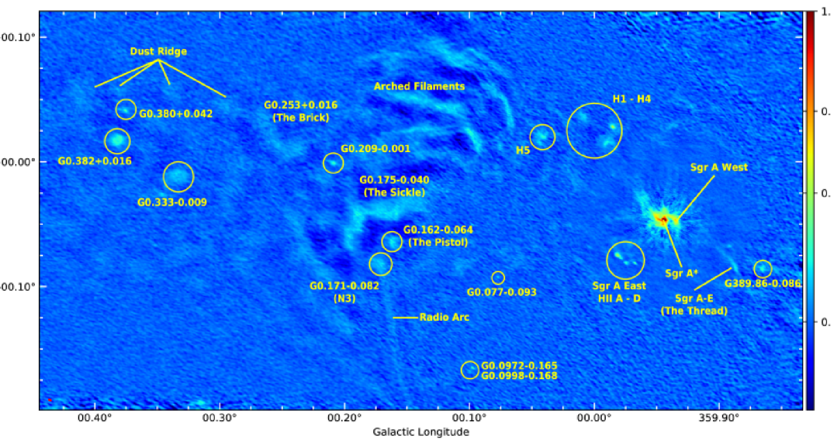
Figure 1: CARMA 15+8 3 mm continuum map with a spatial resolution is $7.62\arcsec\times 3.51\arcsec$ (synthesized beam indicated in red in lower left corner). Prominent features are labeled, including the thermal Arched Filaments, Sickle, Pistol, the Brick, nonthermal radio filaments the Radio Arc and the Thread, Sgr A* and Sgr A West, several HII regions, and the clouds associated with the Dust Ridge.

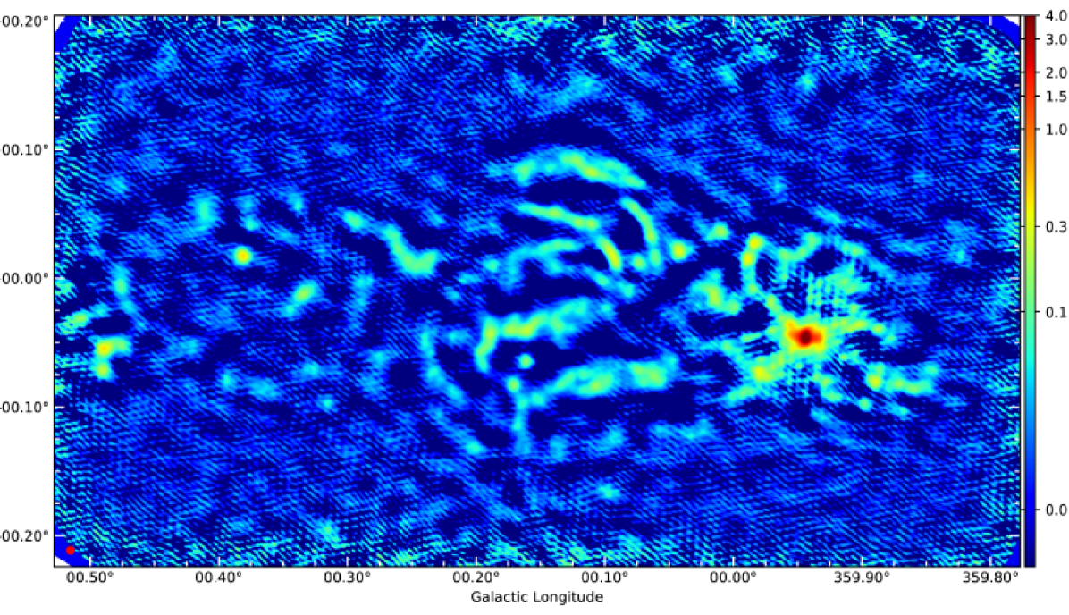
Figure 2: CARMA-8 3 mm continuum map, smoothed to a round 20″ beam (synthesized beam indicated in red in lower left corner). Because of the larger primary beam of the 3.5-m antennas, this map slightly larger than the CARMA 15+8 map displayed in Fig. 1. Diffuse features with surface brightness, such as the Dust Ridge and the Brick, have comparatively higher flux density. There are high frequency striations in the vertical direction near Sgr A*. These are artifacts of CLEANing.

One of the advantages of observing the Galactic Center at 3 mm with CARMA is that it allows identification of different types of emission from this confusing region of the Galaxy. In continuum, we detect emission from dust grains, optically thin free-free emission from ionized gas, synchrotron emission from nonthermal filaments, and ultra-compact HII regions distributed throughout the region.

Because the electron density is proportional to the observed frequency, 3 mm observations are sensitive to compact and ultra-compact (UC) HII regions with high densities. Our 3 mm continuum survey can study the class of compact HII regions with emission measures $\leq 3\times$ $10^{10}$ pc cm^-6 at the turnover frequency $\tau\leq 1$. We detect the chain of compact Sgr A East HII regions, which are the closest massive star forming regions to Sgr A*, and several isolated compact HII regions.

The Galactic Center also hosts two well-known young stellar clusters: the Arches and the Quintuplet clusters. There is an additional cluster of stars, the so-called the central cluster, that orbits Sgr A* (Paumard et al., 2006). Diffuse and bright sources excited by hot members of these young clusters are Sgr A West, the Arched Filaments, and the Sickle, all of which are visible at 3 mm.

The physical characteristics of molecular gas in the CMZ are similar to those of infrared dark clouds (IRDCs). Herschel observations show that IRDCs have low dust temperatures (Pierce-Price et al., 2000; Molinari et al., 2011; Rodríguez & Zapata, 2013). We identify several of these IRDCs in the chain of clouds forming the so-called Dust Ridge (Lis & Carlstrom, 1994; Lis et al., 2001) of molecular gas distributed between G0.253+0.016/ and Sgr B2. G0.253+0.016 has been the focus of numerous recent papers, both suggesting it is the precursor cloud to an Arches-like stellar cluster (Longmore et al., 2012; Rathborne et al., 2015) and that it is not (Kauffmann et al., 2013; Johnston et al., 2014). In Figs. 1 and 2, the cloud is seen with uniform intensity $\sim 0.01$ Jy beam^-1.

Low frequency radio continuum surveys of the Galactic Center show a population of magnetized filamentary structures throughout the CMZ, many of which have a steep spectrum, and thus cannot be detected at 3 mm (Lang et al., 1999; LaRosa et al., 2000; Yusef-Zadeh et al., 1984, 2004). However, some filaments have a flat spectrum, such as the ones in the Radio Arc at $l\sim$0$.\kern-2.5pt^{{}^{\circ}}$2. In Figs. 1 and 2 show clearly the brightest filament running perpendicular to the Galactic plane, passing through nonthermal source N3 (Yusef-Zadeh & Morris, 1987a; Ludovici et al., 2016), through the Sickle, and curving to pass across the Arched Filaments. The mean 3 mm flux density of this filament is 3.5 mJy beam^-1. The origin of these unique flat-spectrum filaments is unknown.

We have measured the parameters at 3 mm for both compact and extended sources. For sources which appeared unresolved or marginally resolved, we used MIRIAD’s imfit task to fit a 2-dimensional Gaussian, excluding from the fit pixels with intensities below the 1$\sigma$ rms noise level measured locally. Such exclusion produced quantitatively better fits to the measured peak intensities than clipping at zero flux density. The deconvolved source size and peak intensity are derived from the Gaussian fit. Brightness temperatures were computed using equation 2.18 of Brown (1987). The low derived brightness temperatures indicate that all of these sources are optically thin at 3 mm. For the compact sources, entries in columns 1-6 respectively of Table 3 list source name, Galactic coordinates, fitted peak intensity, brightness temperature, and fitted source size and position angle. For extended sources, we measured the total flux density in a box around each source, clipping the background at twice the 1$\sigma$ rms noise level which was measured locally (Table 4). Entries in columns 1-5 of Table 4 are source name, Galactic coordinates, total flux density, the size of the box within which the flux was measured, and area of pixels greater than 2$\sigma$ that contribute to the total flux density, respectively. Individual sources are shown in Figs. 3 to 11 and are briefly described below.

Table 3: Parameters of Compact 3 mm Sources. ¹Peak Intensity and deconvolved quantities are derived from Gaussian fit. See §3.1.

	$l$	$b$	Peak Intensity	Brightness Temp.	Deconvolved Size	Deconvolved PA
Source	(∘)	(∘)	(Jy beam-1)	(K)	(″)	(∘)	Fig.
H7	0.0331	+0.0295	0.013 $\pm$ 0.001	0.07 $\pm$ 0.01	7.4 $\times$ 1.1	56.2	5
G0.077-0.093	0.0773	-0.0925	0.028 $\pm$ 0.005	0.16 $\pm$ 0.03	3.6 $\times$ 1.4	26.3	7
G0.075-0.073	0.0749	-0.0726	0.016 $\pm$ 0.002	0.09 $\pm$ 0.01	8.2 $\times$ 4.9	44.8	7
G0.098-0.050	0.0975	-0.0504	0.022 $\pm$ 0.005	0.12 $\pm$ 0.03	7.5 $\times$ 1.4	51.7	7
G0.0972-0.165	0.0972	-0.1654	0.068 $\pm$ 0.007	0.38 $\pm$ 0.04	4.1 $\times$ 1.8	38.3	8
G0.0998-0.168	0.0998	-0.1680	0.014 $\pm$ 0.002	0.08 $\pm$ 0.01	13.7 $\times$ 8.5	37.6	8
G0.209-0.001	0.2083	-0.0012	0.038 $\pm$ 0.003	0.21 $\pm$ 0.02	17.5 $\times$ 9.2	70.8	12
G0.323+0.108	0.3228	+0.0183	0.010 $\pm$ 0.002	0.06 $\pm$ 0.01	15.7 $\times$ 6.5	75.3	10
G0.352-0.067	0.3515	-0.0669	0.015 $\pm$ 0.001	0.08 $\pm$ 0.01	10.8 $\times$ 4.2	78.0	10
G0.380+0.042	0.3802	+0.0418	0.016 $\pm$ 0.002	0.09 $\pm$ 0.01	18.6 $\times$ 7.6	73.6	9

Table 4: Flux Densities of Extended 3 mm Sources. ¹Denotes the area of pixels greater than the cutoff that contribute to the total flux density. ²While this box includes The Pistol, we masked out emission from the Pistol box when measuring the flux of The Sickle.

Source	$l$	$b$	Flux Density	Box size	Area
	(∘)	(∘)	(Jy)	$\Delta~{}l(\arcsec)\times\Delta~{}b(\arcsec)$	(″)
G359.86-0.086	359.8656	-0.0862	0.375 $\pm$ 0.041	61$\times$ 37	709
G359.89-0.068	359.8917	-0.0676	0.052 $\pm$ 0.011	31$\times$ 21	153
SgrA-E	359.8870	-0.0847	0.392 $\pm$ 0.030	79$\times$ 81	1070
Parachute	359.9217	0.0435	0.405 $\pm$ 0.042	101$\times$ 101	1328
Sgr A East HII A/B	359.9815	-0.0751	0.486 $\pm$ 0.020	32$\times$ 32	570
Sgr A East HII C	359.9745	-0.0812	0.107 $\pm$ 0.012	21$\times$ 18	205
Sgr A East HII D	359.9674	-0.0814	0.088 $\pm$ 0.010	23$\times$ 16	164
H1	359.9903	+0.0152	0.510 $\pm$ 0.047	64$\times$ 61	1114
H2	359.9852	+0.0281	0.538 $\pm$ 0.038	56$\times$ 48	721
H3	0.0084	+0.0356	0.272 $\pm$ 0.034	49$\times$ 48	602
H4	0.0223	+0.0297	0.080 $\pm$ 0.022	51$\times$ 61	248
H5	0.0415	+0.0198	0.636 $\pm$ 0.049	51$\times$ 61	1205
H8	359.9853	-0.0110	0.027 $\pm$ 0.009	31$\times$ 26	122
G0.109-0.084	0.1089	-0.0841	0.226 $\pm$ 0.034	81$\times$ 69	756
Arched Filaments	0.125	+0.045	12.073 $\pm$ 0.213	461$\times$ 391	29852
Pistol	0.1618	-0.0644	0.537 $\pm$ 0.034	71$\times$ 61	1251
N3	0.1714	-0.0816	0.686 $\pm$ 0.046	81$\times$ 71	1775
Sickle	0.175	-0.040	6.651 $\pm$ 0.133	271$\times$ 191	14953
G0.333-0.009	0.3331	-0.0086	0.968 $\pm$ 0.052	91$\times$ 66	2579
G0.346-0.026	0.3460	-0.0260	0.182 $\pm$ 0.024	55$\times$ 36	537
G0.375+0.041	0.3754	+0.0408	0.243 $\pm$ 0.023	52$\times$ 28	519
G0.382+0.016	0.3820	+0.0164	1.193 $\pm$ 0.043	83$\times$ 66	1829

3.1.1 Notes On Individual Continuum Sources

Sgr A* and Sgr A West

The mini-spiral HII region in Figure 3 shows three arms of ionized gas orbiting Sgr A*. Low-frequency emission from the southern arm of the mini-spiral seen to the west is optically thick (Yusef-Zadeh et al., 2004), whereas the emission at 3mm is most likely a mixture of dust and ionized gas. Recent ALMA observations of the mini-spiral show clearly that cool dust dominates the emission at submm wavelengths (Tsuboi et al., 2016).

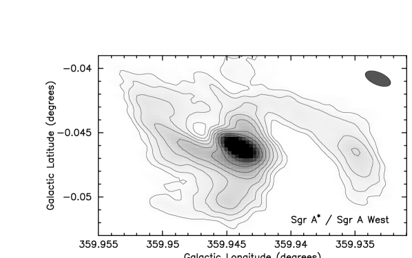
Figure 3: 3 mm continuum map of Sgr A* and Sgr A West aka the mini-spiral. The peak flux intensity of Sgr A* is 2.8 Jy beam^-1. Contours are at 0.080, 0.114, 0.163, 0.232, 0.332, 0.473, 0.675, 0.964, 1.38, 1.96, 2.80 Jy beam^-1 (1$\sigma$ rms noise is 0.002 Jy beam^-1). The grayscale ranges from 0.05 to 1.5 Jy beam^-1. In this and the following figures, the synthesized beam is shown in the upper right corner.

Sgr A East A-D (Fig. 4)

The Sgr A East A-D complex of compact HII regions was first noted by Ekers et al. (1983). These HII regions photoionized by young O8-B0 stars are associated with the 50 ${\rm km~{}s^{-1}}$ molecular cloud (Yusef-Zadeh et al., 2010; Mills et al., 2011, and references therein). At 3 mm, sources A, B, and D appear centrally peaked, while source C has a peak offset to the east. The peak is coincident with 6 cm source C1 and the broadening towards the west coincident with 6 cm source C2 (Yusef-Zadeh & Morris, 1987b).

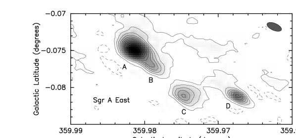
Figure 4: 3 mm continuum map of the Sgr A East A-D complex of compact HII regions. Contours are in steps of $4\sigma$ from -2$\sigma$ to 46$\sigma$, where the 1$\sigma$ rms noise is 0.002 Jy beam^-1. The grayscale ranges from 0.005 to 0.1 Jy beam^-1.

Sources H1 through H8 (Fig. 5)

H1 through H5 are known to be HII regions and at 3 mm their morphologies correspond well to 6 cm continuum maps (Yusef-Zadeh & Morris, 1987b; Zhao et al., 1993). H1 has a shell-like morphology, while H2 is very bright and compact with a narrow, $\sim 25\arcsec$-long ridge to the south. H4 is a comparatively weak shell with a $\sim 40\arcsec$-long low intensity extension to the north. H5 breaks up into bright east and west components surrounded by lower intensity emission. A hint of the 6 cm tongue of emission extending southward is seen at 3 mm. H7 appears as a compact sources H7 (intensity per unit frequency $I_{\nu}=13\pm 1$ mJy beam^-1). H8 ($S_{\nu}=27\pm 9$ mJy) is resolved with a slight extension westwards. We also see in this region broad-scale, low intensity emission at positive Galactic longitude that is similar to features seen at 6 cm.

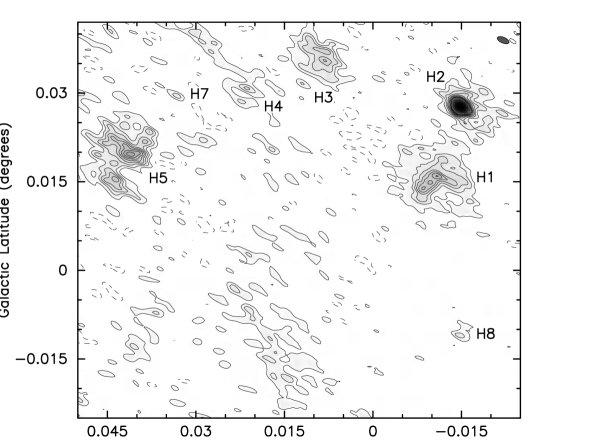
Figure 5: 3 mm continuum image of sources H1 through H8 (H6 was not detected). Contours are at -0.0075, 0.005, 0.01, 0.015, 0.02, 0.025, 0.03, 0.035, 0.04, 0.045, 0.055, 0.065, 0.075, 0.085, 0.095, 0.105, 0.115, 0.125 Jy beam^-1. The $1\sigma$ rms noise is 0.002 Jy beam^-1 and the grayscale ranges from 0.005 to 0.12 Jy beam^-1.

Sources SgrA-E, G359.89-0.068, and G359.86-0.086 (Fig. 6)

SgrA-E is a nonthermal filament associated with X-ray source XMM J174540-2904.5 and believed to be interacting with a molecular cloud (Yusef-Zadeh et al., 2005). In our map, it is nearly 100″  long with a peak intensity of 0.028 Jy beam^-1. The brightest region in 3 mm ($-0.09^{\circ}\la b\la-0.08^{\circ}$) corresponds to the regions of most intense 2 cm and X-ray emission.

G359.89-0.068 is a compact 3 mm source, coincident with submillimeter source JCMTSF J174537.6-290350 from the SCUBA survey catalog of Di Francesco et al. (2008) that has an 850 µm flux density of 9.62 Jy. We find no counterpart to G359.89-0.068 at 2 cm or 6 cm. G359.86-0.086, also known as SgrA-G, is an HII region (Ho et al., 1985; Yusef-Zadeh & Morris, 1987b) near the edge of a bright submillimeter cloud in the SCUBA map. At 3 mm, it is centrally peaked with a maximum intensity of 0.047 Jy beam^-1 and at 2 cm, the source appears clumpy, possibly shell-like (Ho et al., 1985).

Figure 6: Continuum 3 mm close-up of sources SgrA-E (also known as “The Thread”), G359.89-0.068, and G359.86-0.086. The $1\sigma$ rms noise in this map is about 0.003 Jy beam^-1 (somewhat lower near SgrA-E, somewhat higher near G359.89-0.068). Contours are -0.007, 0.007, 0.014, 0.021, 0.028, 0.035, 0.042 Jy beam^-1 and the grayscale ranges from 0.0035 to 0.05 Jy beam^-1.

Sources G0.075-0.073, G0.077-0.093, G0.098-0.050, and G0.109-0.084 (Fig. 7)

In our 3 mm map, G0.075-0.073, G0.077-0.093 and G0.098-0.050 are isolated, unresolved sources, with peak intensities between 16 and 28 mJy beam^-1. G0.077-0.093 and G0.098-0.050 are identified as compact sources B1 and C1, respectively, in Toomey (2014) with varying spectral indices between 2.8 GHz and 5.3 GHz. G0.077-0.093 appears in the 2LC catalog (Lazio & Cordes, 2008) with a 1.4 GHz flux density of 0.00292 Jy. It is also 1.6″ from Chandra source CXOGCS J174609.7-285505 (Muno et al., 2006). We find no clear match for G0.098-0.050 in the SIMBAD database.

G0.109-0.084 is a diffuse, low intensity source with a peak intensity of 0.015 Jy beam^-1, while G0.075-0.073 is a compact peak in a more diffuse region. These two diffuse regions coincide with BGPS G000.106-00.085 and BGPS G000.066-00.079, respectively, which in the BOLOCAM 1.1 mm survey image are teardropped shaped peaks within more extended nebulosity. The 1.1 mm flux density of BGPS G000.106-00.085 is $13.584\pm 0.88$ Jy and of BGPS G000.066-00.07 is $11.237\pm 0.723$ Jy (Rosolowsky et al., 2010). G0.075-0.073 is coincident with the narrow end of the BGPS G000.066-00.079 “teardrop” and may represent an embedded source or simply a local peak. These diffuse clouds are clearly seen in the CARMA-8 map (Fig. 2).

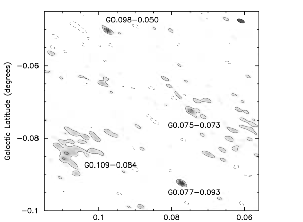
Figure 7: The 3 mm continuum map of G0.075-0.073, G0.077-0.093, G0.098-0.050, and G0.109-0.084. Contours are -0.007, 0.007, 0.014, 0.021 Jy beam^-1. The $1\sigma$ rms is 0.0035 Jy beam^-1 and the grayscale ranges from 0.005 to 0.035 Jy beam^-1.

Sources G0.0972-0.165 and G0.0998-0.168 (Fig. 8)

G0.0972-0.165 and G0.0998-0.168 correspond to sources A1 and A2, respectively, in Toomey (2014). They are both unresolved at 3 mm. They coincide with the unresolved BOLOCAM source BGPS G000.098-00.163, which has a 1.1 mm flux density of $1.272\pm 0.133$ Jy. At 4.8GHz, G0.0998-0.168 appears as a clumpy shell about 12″ in diameter (Toomey, 2014).

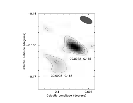
Figure 8: The 3 mm CARMA15+8 continuum map of G0.0972-0.165 and G0.0998-0.168 corresponding to sources A1 and A2, respectively, in Toomey (2014). Contours are 0.008, 0.016, 0.024, 0.032, 0.040, 0.048, 0.056, 0.064 Jy beam^-1. The $1\sigma$ rms is 0.004 Jy beam^-1 and the grayscale ranges from 0.004 to 0.06 Jy beam^-1.

Sources G0.382+0.016 and G0.375+0.041 (Fig. 9)

G0.382+0.016 has been variously classified as an HII region based on radio recombination and HI spectral lines (Anderson et al., 2011), as an UC HII region based on IRAS colors (Becker et al., 1994), and as a supernova remnant (LaRosa et al., 2000). In the 870 µm and 8.4 GHz continuum surveys of Immer et al. (2012), it is identified as Source E. With an integrated flux density of 1.193 Jy, is one of the brightest continuum sources in our 3 mm survey, with a clear shell structure. Assuming $S_{\nu}\propto\nu^{\alpha}$, the spectral index $\alpha$ is defined as $\alpha=\log(S_{1}/S_{2})/\log(\nu_{1}/\nu_{2})$. Using the flux density at 9 GHz of 1.513$\pm$0.053 Jy and our 90 GHz measurement (Table 4), we derive a spectral index $\alpha=-0.10\pm 0.05$ (where $\alpha=\log(S_{1}/S_{2})/\log(\nu_{1}/\nu_{2})$, given $S_{\nu}\propto\nu^{\alpha}$), consistent with optically thin free-free emission and thus supporting the identification as an HII region. G0.375+0.041 is coincident with maser features (e.g., Caswell et al., 1995; Argon et al., 2000) and Spitzer source SSTGC 639320, and is classifed as a YSO by Yusef-Zadeh et al. (2009). At 3 mm, it is resolved into two compact sources with a common envelope of emission. The brighter of these has a peak intensity of 0.07 Jy beam^-1, the weaker 0.02 Jy beam^-1.

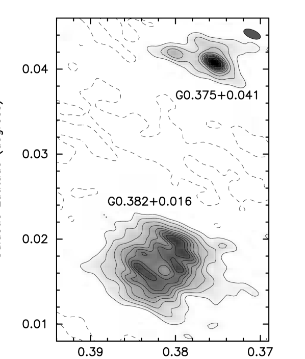
Figure 9: Sources G0.382+0.016 and G0.375+0.041. Contours are -0.0056, 0.0056, 0.0112, 0.0168, 0.0224, 0.028, 0.0336, 0.0392, 0.0448, 0.056, 0.0672 Jy beam^-1. The $1\sigma$ rms noise is 0.0028 Jy beam^-1 and the grayscale ranges from 0.003 to 0.06 Jy beam^-1.

Sources G0.352-0.067 and G0.323+0.0108 (Fig. 10)

G0.352-0.067 is an isolated, compact 3 mm source with peak intensity of 0.015 Jy beam^-1 . It appears in the 2LC catalog (Lazio & Cordes, 2008) with angular diameter of 2″ and 1.4 GHz flux density of 0.0277 Jy. At 5 GHz, it has flux density of 0.0224 Jy (Becker et al., 1994). G0.323+0.0108 is also compact and isolated at 3 mm with a peak intensity of 0.010 Jy beam^-1. We find no lower frequency radio counterpart within 30″ of G0.323+0.0108 in the SIMBAD database. An extended submillimeter source JCMTSE J174620.3-283931 is centered 12.2″ away with a total 850 µm flux density of 0.53 Jy (Di Francesco et al., 2008). The position of G0.323+0.0108 is coincident with a small tongue of emission extending from JCMTSE J174620.3-283931. However, there is no 3 mm emission associated with JCMTSE J174620.3-283931 in the CARMA-8 map, which is more sensitive to extended structure.

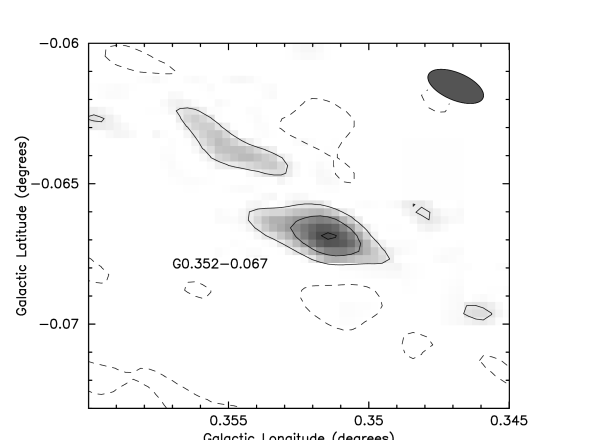
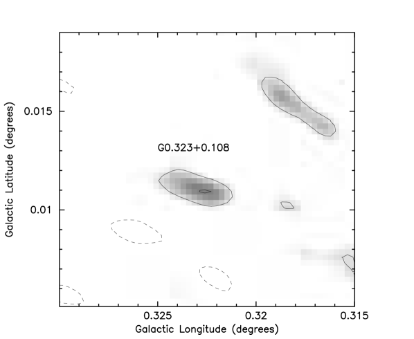
Figure 10: Sources G0.352-0.067 (top) and G0.323+0.108 (bottom). For G0.352-0.067, contours are -0.005, 0.005, 0.01, 0.015 Jy beam^-1, the $1\sigma$ rms noise is 0.0025 Jy beam^-1, and the grayscale ranges from 0.003 to 0.02 Jy beam^-1. For G0.323+0.108 contours are -0.006, 0.006, 0.012 Jy beam^-1, the $1\sigma$ rms noise is 0.003 Jy beam^-1, and the grayscale ranges from 0.004 to 0.02 Jy beam^-1.

The Sickle, The Pistol, and N3 (Fig. 11)

The nonthermal radio filaments of the Arc appear to cross the sickle and the Galactic plane. There are two prominent HII regions G0.18-0.04 (The Sickle nebula) and G0.16-0.06 (the Pistol nebula). These nebulae lie in the region of the Quintuplet Cluster, a young cluster of massive stars in the Galactic Center. The radio source N3 (G0.171-0.082) appears in Fig. 1 to be crossed by the Radio Arc as is also seen in maps at lower frequencies (Yusef-Zadeh & Morris, 1987a; Ludovici et al., 2016). Between 4.5 and 49 GHz, N3 is a point source (Ludovici et al., 2016); however at 3mm we see extended emission surrounding the point source location that coincides with one of the 3 mm contour peaks. The extended continuum emission is coincident with the interacting molecular cloud identified by (Ludovici et al., 2016) which we also clearly detect in CS, SiO, and HCN, and weakly detect in HCO⁺ and N₂H⁺ (Figs. 14 to 18).

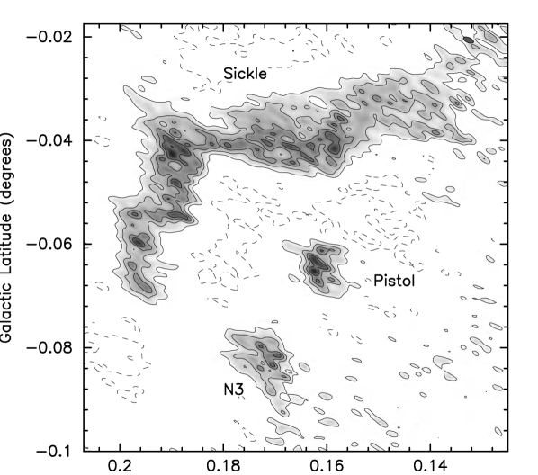
Figure 11: The 3 mm CARMA15+8 continuum map of region of the Sickle, the Pistol, and N3. Contours are -0.009, 0.006, 0.012, 0.018, 0.024 Jy beam^-1. The $1\sigma$ rms is 0.003 Jy beam^-1 and the grayscale ranges from 0.005 to 0.04 Jy beam^-1.

Source G0.209-0.001 (Fig. 12)

G0.209-0.001 is a compact source north of the Sickle with a peak 3 mm flux density of 0.05 Jy beam^-1. It has a slightly curved, lower emissivity ($\sim$0.01 Jy beam^-1) north-south extension. Lang et al. (2010) measure a 1.4 GHz flux density of 0.447$\pm$0.032 Jy. It is identified as source D1 in Toomey (2014) with a varying spectral index between 2.8 and 5.3 GHz, as SCUBA source JCMTF J174606.9-284536 with a flux density of 4.14 Jy (Di Francesco et al., 2008), and BOLOCAM source BGPS G000.208-00.003 with a 1.1mm (268 GHz) flux density of 1.506$\pm$0.14 Jy (Rosolowsky et al., 2010). Hill et al. (2005) note the source is coincident with both radio continuum emission and with a methanol maser with radial velocity $V=42.1-49.4~{}{\,{\rm km~{}s^{-1}}}$ (Walsh et al., 1998), and is identified as an UC HII region at a distance of 7.36 kpc (Walsh et al., 2003). Its total 3 mm flux density is 0.227 $\pm$ 0.024 Jy, giving a spectral index values $\alpha=-0.16\pm 0.07$ and $1.7\pm 0.2$ measured between 1.4 – 90 GHz and 90 – 268 GHz, respectively.

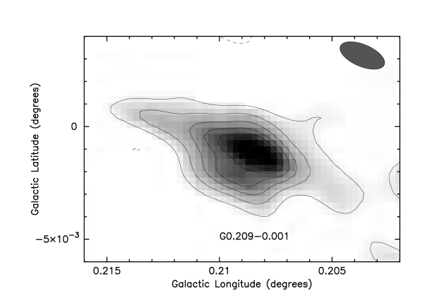
Figure 12: CARMA 3 mm continuum map of G0.209-0.001. Contour levels are set at -0.006, 0.006, 0.012, 0.018, 0.024, 0.030, 0.036, 0.042, 0.048 Jy beam^-1. The $1\sigma$ rms is 0.003 Jy beam^-1 and the grayscale ranges from 0.004 to 0.04 Jy beam^-1.

Sources G0.333-0.009 and G0.346-0.026 (Fig. 13)

G0.333-0.009 is roughly circular and has a clumpy, shell morphology with integrated flux density of 0.968$\pm$0.052 Jy at 3 mm. At 1.4 GHz it has a total flux density of 1.618$\pm$0.101 Jy (Lang et al., 2010), giving a spectral index to 90 GHz of $\alpha=-0.12\pm 0.05$. This source is likely an HII region. G0.346-0.026 is listed with a 1.4 GHz flux density of 0.178$\pm$0.028 Jy in Lang et al. (2010), a 5 GHz flux density of 0.080$\pm$0.024 Jy in Becker et al. (1994), and categorized as a YSO candidate by Felli et al. (2002). In our 3 mm map, the source has a central peak intensity of 0.026 Jy beam^-1 and is elongated north-south.

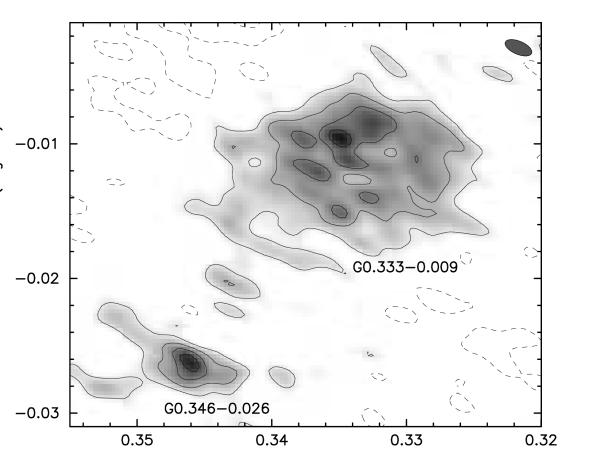
Figure 13: Sources G0.333-0.009 and G0.346-0.026. Contours are -0.0056, 0.0056, 0.0112, 0.0168, 0.0224 Jy beam^-1. The $1\sigma$ rms noise is 0.0028 Jy beam^-1 and the grayscale ranges from 0.003 to 0.03 Jy beam^-1.

3.2 3 mm Spectral Line Data

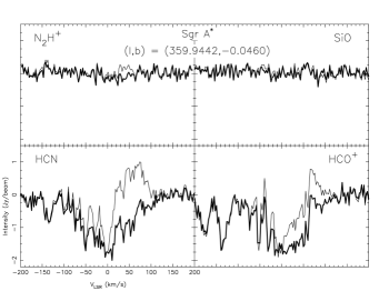
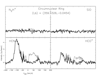
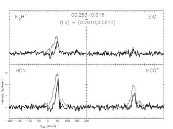
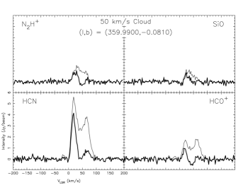
Figure 35: Example spectra from four regions in the CMZ, clockwise from upper left: Sgr A*, the circumnuclear ring (centered on position I in fig. 8 of Wright et al. (2001)), the 50 ${\rm km~{}s^{-1}}$ cloud, and G0.253+0.016. Spectra are averages of 11″$\times$ 11″ boxes centered on the Galactic coordinates shown in each panel.Bold lines are CARMA-15 interferometric data, while thin lines are CARMA-15 plus Mopra data.

We present integrated intensity maps from both the CARMA-15 (Figs. 14 to 18) and CARMA-15 plus Mopra data cubes (Figs. 19 to 26). In maps containing only CARMA data, compact clouds and patches of diffuse features are detected whereas, the combined maps, additional large scale diffuse emission is revealed. In the channel maps (Figs. 19 to 22), molecular emission is detected from a number of Galactic Cener clouds such as G0.253+0.016 (“The Brick”), G0.13-0.13, the 20 ${\rm km~{}s^{-1}}$ and 50 ${\rm km~{}s^{-1}}$ clouds, and the 2–7 pc circumnuclear ring orbiting Sgr A*. In addition, we find a wealth of fine scale filamentary structure throughout the region. Also seen are HCO⁺ and HCN absorption features between ${\rm V_{LSR}}\sim-140-100{\,{\rm km~{}s^{-1}}}$ at the position of Sgr A*, as previously reported by Wright et al. (2001) (see also upper left panel of Fig. 35).

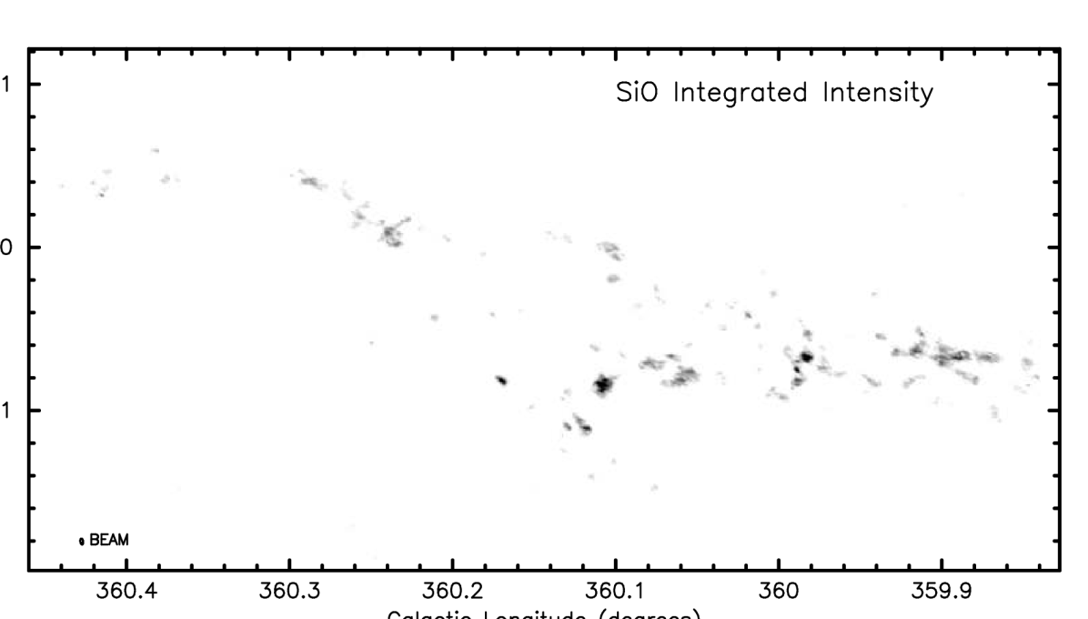
Figure 14: Intensity of SiO(J=2-1) integrated between V_LSR= 0-60 ${\rm km~{}s^{-1}}$. This map contains only CARMA-15 interferometric data. The grayscale range is 0 to 17 Jy beam^-1 ${\rm km~{}s^{-1}}$. The synthesized beam, measuring 13$.\negthinspace^{\prime\prime}$1″$\times$ 5$.\negthinspace^{\prime\prime}$9 is indicated in the lower left corner.

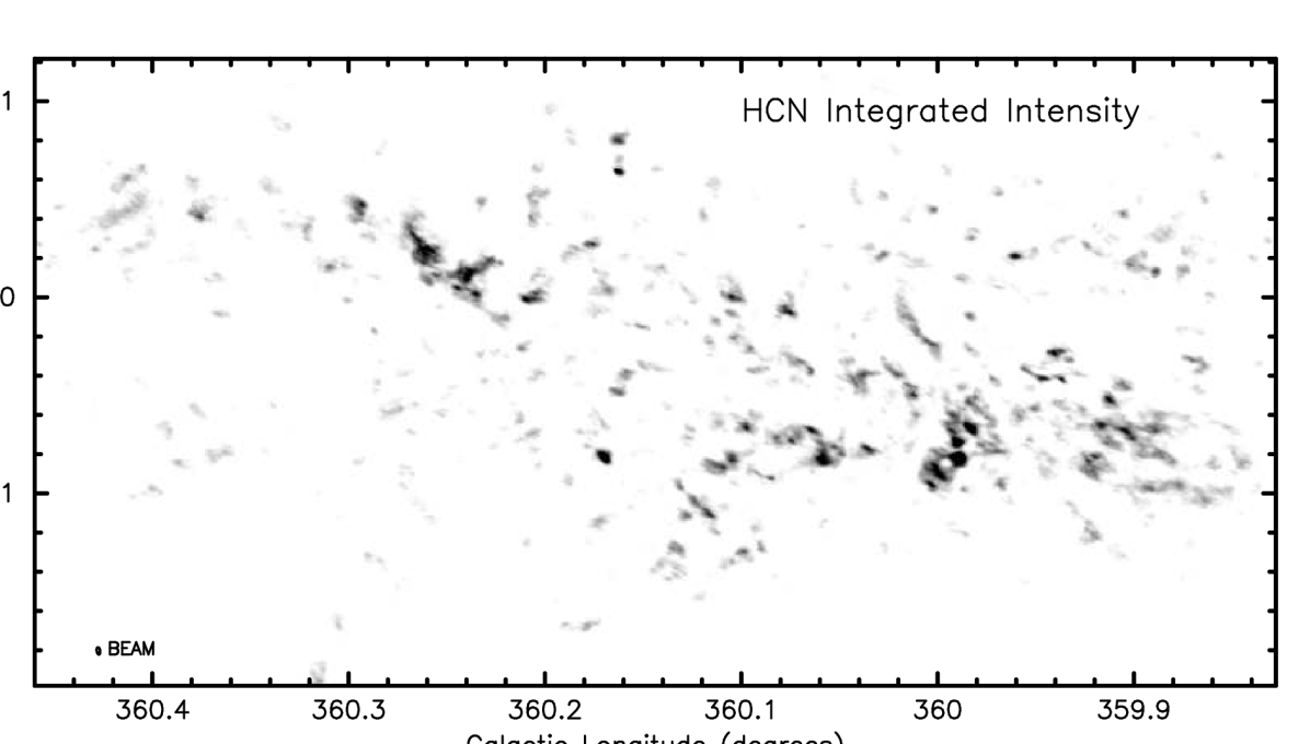
Figure 15: Intensity of HCN(J=1-0) integrated between V_LSR= 0-60 ${\rm km~{}s^{-1}}$. This map contains only CARMA-15 interferometric data. The grayscale range is 1 to 40 Jy beam^-1 ${\rm km~{}s^{-1}}$. The synthesized beam, measuring 13$.\negthinspace^{\prime\prime}$2″$\times$ 5$.\negthinspace^{\prime\prime}$9 is indicated in the lower left corner.

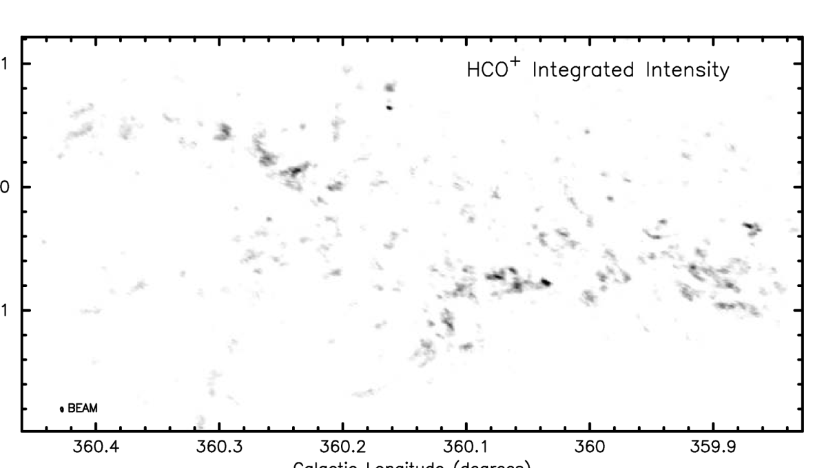
Figure 16: Intensity of HCO⁺(J=1-0) integrated between V_LSR= 0-60 ${\rm km~{}s^{-1}}$. This map contains only CARMA-15 interferometric data. The grayscale range is 1 to 40 Jy beam^-1 ${\rm km~{}s^{-1}}$. The synthesized beam, measuring 13$.\negthinspace^{\prime\prime}$1″$\times$ 5$.\negthinspace^{\prime\prime}$9 is indicated in the lower left corner.

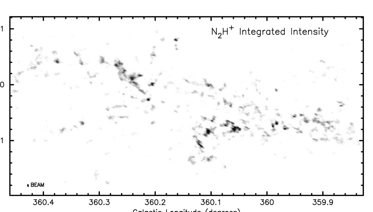
Figure 17: Intensity of N₂H⁺(J=1-0) integrated between V_LSR= 0-60 ${\rm km~{}s^{-1}}$. This map contains only CARMA-15 interferometric data. The grayscale range is 1 to 40 Jy beam^-1 ${\rm km~{}s^{-1}}$. The synthesized beam, measuring 12$.\negthinspace^{\prime\prime}$3″$\times$ 5$.\negthinspace^{\prime\prime}$6 is indicated in the lower left corner.

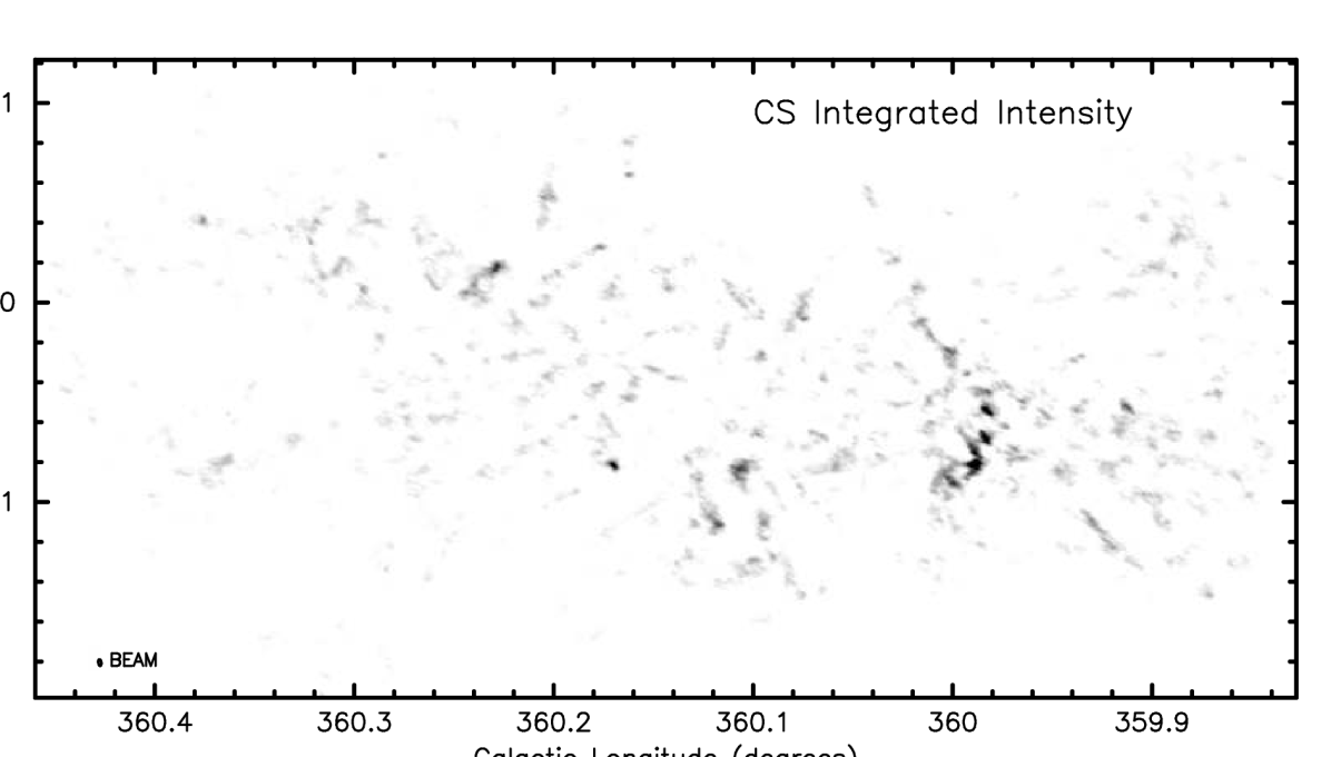
Figure 18: Intensity of CS(J=2-1) integrated between V_LSR= 0-60 ${\rm km~{}s^{-1}}$. This map contains only CARMA-15 interferometric data. The grayscale range is 2 to 50 Jy beam^-1 ${\rm km~{}s^{-1}}$. The synthesized beam, measuring 11$.\negthinspace^{\prime\prime}$8″$\times$ 5$.\negthinspace^{\prime\prime}$3 is indicated in the lower left corner.

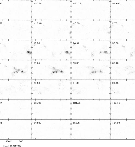
Figure 19: Channel maps of SiO(J=2-1) of the combined CARMA-15 plus Mopra data. Panels are three channel averages with center LSR velocity indicated in upper left of each panel. The grayscale range is 0.2 to 1.3 Jy beam^-1. The spatial resolution is 13$.\negthinspace^{\prime\prime}$1″$\times$ 5$.\negthinspace^{\prime\prime}$9.

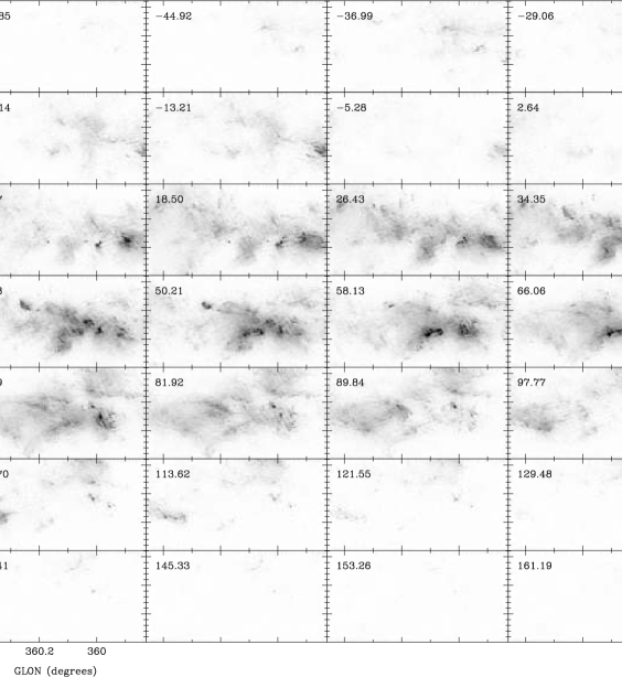
Figure 20: Channel maps of HCN(J=1-0) of the combined CARMA-15 plus Mopra data. Panels are three channel averages with center LSR velocity indicated in upper left of each panel. The grayscale range is 0.1 to 4 Jy beam^-1. The spatial resolution is 13$.\negthinspace^{\prime\prime}$2″$\times$ 5$.\negthinspace^{\prime\prime}$9″.

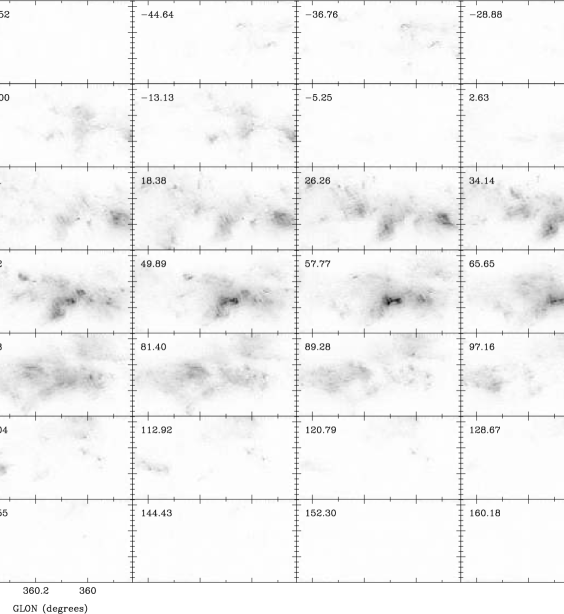
Figure 21: Channel maps of HCO⁺(J=1-0) of the combined CARMA-15 plus Mopra data. Panels are three channel averages with center LSR velocity indicated in upper left of each panel. The grayscale range is 0.1 to 4 Jy beam^-1. The spatial resolution is 13$.\negthinspace^{\prime\prime}$1″$\times$ 5$.\negthinspace^{\prime\prime}$9″.

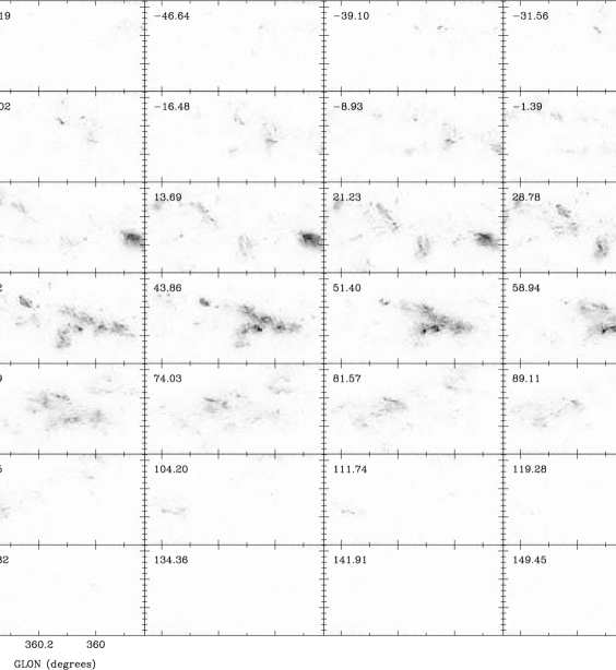
Figure 22: Channel maps of N₂H⁺(J=1-0) of the combined CARMA-15 plus Mopra data. Panels are three channel averages with center LSR velocity indicated in upper left of each panel. The grayscale range is 0.1 to 2.75 Jy beam^-1. The spatial resolution is 12$.\negthinspace^{\prime\prime}$3″$\times$ 5$.\negthinspace^{\prime\prime}$6″.

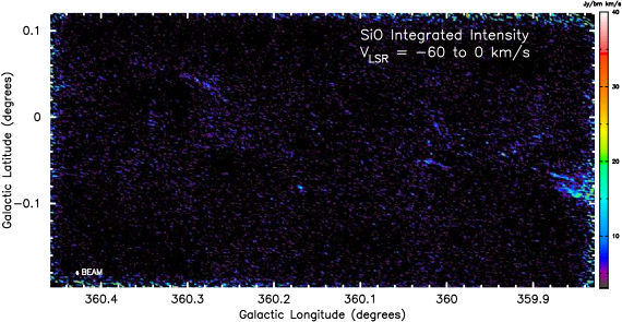
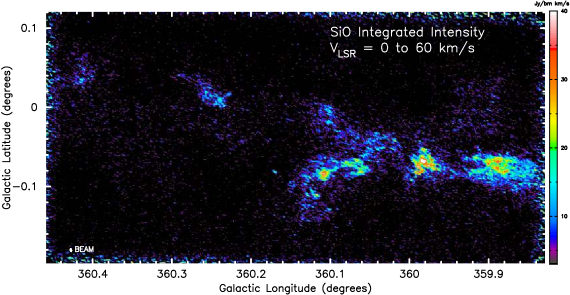
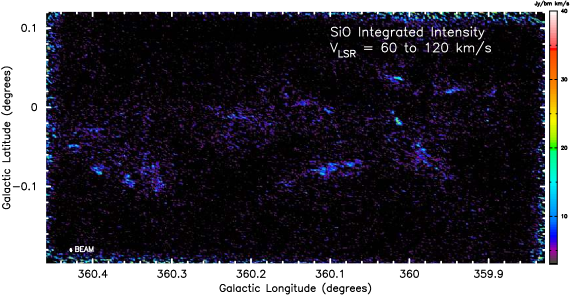
Figure 23: SiO(J=2-1) integrated intensity of the CARMA-15 plus Mopra data. Panels show integrals over selected velocity intervals: top) V_LSR= –60 to 0 ${\rm km~{}s^{-1}}$; middle) V_LSR= 0 to 60 ${\rm km~{}s^{-1}}$; bottom) V_LSR= 60 to 120 ${\rm km~{}s^{-1}}$. The color wedge indicates map intensity values.

Figs. 23 to 26 show intensity maps integrated over 60 ${\rm km~{}s^{-1}}$ wide intervals covering the bulk of the emission in the data cubes. The data were clipped at twice the relevant 1$\sigma$ rms noise indicated in Table 1 before integration. The SiO(J=2-1) emission is the weakest, principally seen only in the range ${\rm V_{LSR}}=0-60$ ${\rm km~{}s^{-1}}$ and in only the region where HCN emission is strongest. The HCN and HCO⁺ emission are brightest with large regions of diffuse emission. The N₂H⁺ emission, in which individual clouds are most easily distinguished, has brightness intermediate between SiO(J=2-1) and HCO⁺.

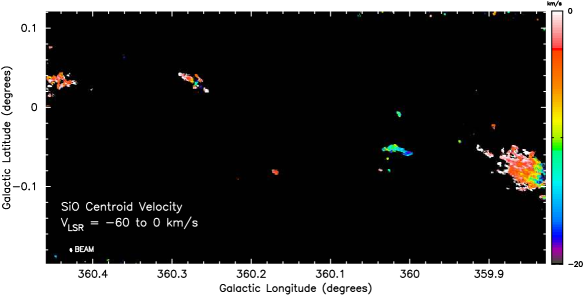
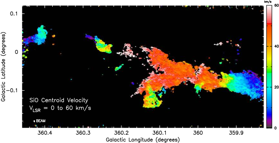
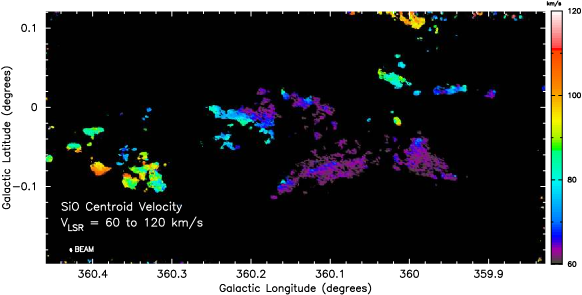
Figure 27: SiO(J=2-1) centroid velocity of the CARMA-15 plus Mopra data. Panels show integrals over selected velocity intervals: top) V_LSR= -60 to 0 ${\rm km~{}s^{-1}}$; middle) V_LSR= 0 to 60 ${\rm km~{}s^{-1}}$; bottom) V_LSR= 60 to 120 ${\rm km~{}s^{-1}}$; and the color wedge indicates map centroid velocity values.

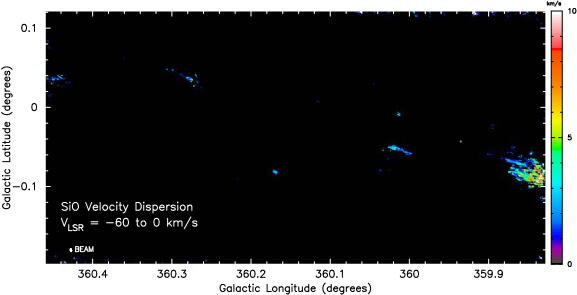
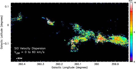
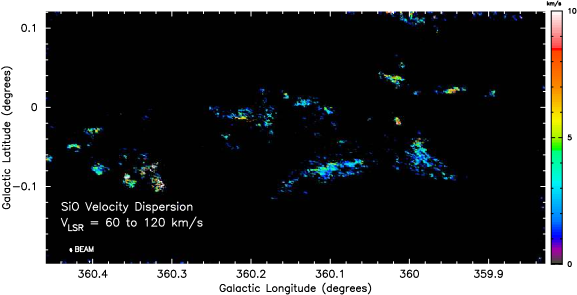
Figure 31: SiO(J=2-1) one-dimensional velocity dispersion of the CARMA-15 plus Mopra data. Panels show integrals over selected velocity intervals: top) V_LSR= -60 to 0 ${\rm km~{}s^{-1}}$; middle) V_LSR= 0 to 60 ${\rm km~{}s^{-1}}$; bottom) V_LSR= 60 to 120 ${\rm km~{}s^{-1}}$; and the color wedge indicates map velocity dispersion values.

Figs. 27 to 30 display the mean velocity (first moment) in each of the spectral lines and Figs. 31 to 34 display the one-dimensional velocity dispersion (second moment). We formed these moment maps using the “smooth-and-mask” technique described by Helfer et al. (2003). This technique can reveal low-level emission better than can be accomplished by simply calculating the moments using a fixed clip level, and furthermore does not bias the noise statistics of the final image. The purpose of this technique is to identify which pixels in a data cube should be included in the moment calculations and which should not. This is done by spatially smoothing the data cube to bring out low S/N emission, then using that smoothed version of the data cube to determine which pixels should be included in the moments (i.e., included in the mask). For each of our spectral line data cubes, a mask was made by spatially smoothing the data with a Gaussian with FWHM = 20″ and then including in the mask the pixels where the intensity in the smoothed data was greater than 3 times the rms noise determined from emission-free channels. Pixels that were isolated on the velocity axis were eliminated from the mask to remove anomalous spikes outside the velocity range of the main emission, which can skew the integrated quantities. The moments of the unsmoothed data were then computed using only pixels that fell within the mask.

In computing the moment maps, we have not attempted to deconvolve the three hyperfine components of HCN  which span $\sim$3.5 MHz or about 4.5 spectral channels, nor the seven hyperfine components of N₂H⁺, which span $\sim$4.7 MHz or about 6 spectral channels. The large line widths of gas in the CMZ obscure much of the hyperfine structure and the similarity between the HCN and HCO⁺ moments suggests that the contamination to these quantities from the hyperfine lines is not significant. We note that G0.253+0.016 stands out as having high velocity dispersion ($\sim 15{\,{\rm km~{}s^{-1}}}$) in N₂H⁺; this may be due to the multiple velocity components noted by Kauffmann et al. (2013).

Example spectra, both with and without the Mopra data added, are shown in Fig. 35. In compact regions, the CARMA-15 data capture the entirety of the emission of the feature with the additional Mopra data providing only the large scale foreground or background components. For instance, the spectra of the circumnuclear ring (Fig. 35, upper right) are centered on component I in fig. 8 of Wright et al. (2001). This portion of the ring emits between ${\rm V_{LSR}}=-150$ to $-50{\,{\rm km~{}s^{-1}}}$ which the CARMA data (bold line) fully recover. However, at positive velocities there is significant HCN and HCO⁺ emission, likely from the 50 ${\rm km~{}s^{-1}}$ cloud, that is mostly seen in the Mopra data (thin line). This emission is not detected by the interferometer because it spatially smooth on the scale of $\sim 30\arcsec$. In the spectra at the position of Sgr A* (Fig. 35, upper left), emission from the 50 ${\rm km~{}s^{-1}}$ cloud is seen to “fill in” the HCN and HCO⁺ absorption features, and is weakly visible in N₂H⁺.

In larger regions, such as G0.253+0.016 (Fig. 35, lower left) and the 50 ${\rm km~{}s^{-1}}$ cloud (Fig. 35, lower right) , the Mopra data increase the line width and peak intensity, or add velocity components. Towards G0.253+0.016, the spectrum is located on a bright core near the center of cloud. Adding the Mopra data detects more of the blueshifted, low emissivity, spatially smoother gas, and enhances the HCN and HCO⁺ feature associated with a line-of-sight cloud at 75 ${\rm km~{}s^{-1}}$ (Rathborne et al., 2014, 2015). The 50 ${\rm km~{}s^{-1}}$ cloud is similarly a complex region with emission at several spatial scales and velocities. These spectra show the importance of recovering all spatial scales when analyzing such regions.

3.3 Correlations with 6.4 keV Iron Fluorescence

Remarkably, the CMZ molecular clouds emit fluorescent Fe K$\alpha$ line emission at 6.4 keV (Koyama et al., 1996). One of our key motivations for mapping the CMZ in different molecular species is to examine the relationship between the distribution of the molecular line emission, the 6.4 keV line emission, and nonthermal radio emission. Broadly, there are two proposed production mechanisms for the 6.4 keV Fe K$\alpha$ emission: the irradiation of molecular cloud by X-rays Ponti et al. (2010) or the impact of 100 MeV cosmic ray electrons with molecular gas (Yusef-Zadeh et al., 2002). In the X-ray model, a molecular cloud is subjected to strong external X-ray radiation which is absorbed and reemited in flourescent iron lines. This model requires past X-ray flares from Sgr A* with $L_{x}\sim 10^{39}~{}{\rm erg~{}s^{-1}}$ (Koyama et al., 1996; Murakami et al., 2000; Murakami et al., 2001; Ponti et al., 2010). A principal piece of evidence for this view is the observed short-term variability ($\sim 10$ years) of X-ray bright spots (Ponti et al., 2010; Soldi et al., 2014).

The cosmic ray picture requires metallicity which is 2-3 times solar. However, it is consistent with enhanced cosmic ray density and a high cosmic ray ionization rate, as traced in radio, infrared and $\gamma$-ray observations of the Galactic Center (Yusef-Zadeh et al., 2002). The electron population from diffuse synchrotron emitting relativistic particles interacting with molecular gas can heat and ionize molecular gas. In addition, Fe K$\alpha$ line emission from neutral iron atoms can be produced by low-energy ($<100$ MeV) cosmic ray bombardment of neutral gas. A three-way spatial correlation between the distributions of molecular gas, nonthermal radio continuum as the source of cosmic rays, and the 6.4 keV line emission is expected in the context of the cosmic ray picture. Our data reveal just such a correlation.

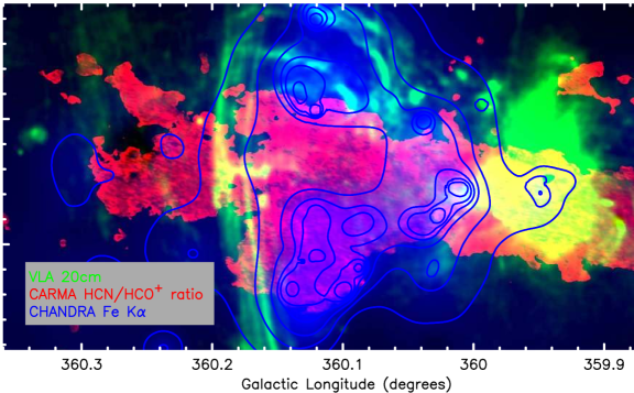
Figure 36: Three-color composite showing ratio of integrated intensities I(HCN)/I(HCO⁺) integrated between V_LSR= 0 to 60 ${\rm km~{}s^{-1}}$ [red] overlaid with 6.4KeV Fe K$\alpha$ intensity [blue], and 20 cm radio continuum [green]. To form the ratio I(HCN)/I(HCO⁺), we divided the maps shown in Figs. 24 and 25, clipping where the I(HCO⁺)$<0.1$ to avoid spuriously large values. The halftone range of I(HCN)/I(HCO⁺) is 0.1 to 2.0 Jy beam^-1 ${\rm km~{}s^{-1}}$ and the halftone range of the 20 cm image is 0 to 0.1 Jy beam^-1. Contours of Fe K$\alpha$ equivalent width are 150, 225, 300, 375, 450, 600 eV. A clear anti-correlation is seen between I(HCN)/I(HCO⁺) and EW(Fe K$\alpha$) in the region bounded by the nonthermal radio emission. This anti-correlation is explored further in Fig. 38.

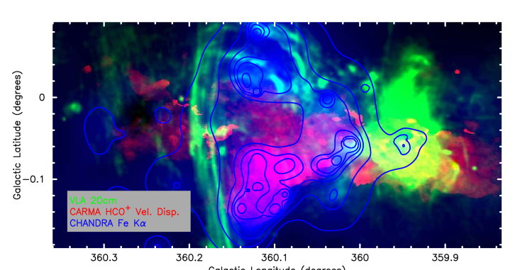
Figure 37: Three-color composite showing velocity dispersion of HCO⁺(J=1-0) [red] overlaid with 6.4KeV Fe K$\alpha$ intensity [blue], and 20 cm radio continuum [green]. The halftone range of the velocity dispersion image is 2 to 15 ${\rm km~{}s^{-1}}$ and the halftone range of the 20 cm image is 0 to 0.1 Jy beam^-1. Contours of Fe K$\alpha$ equivalent width are 150, 225, 300, 375, 450, 600 eV. In the region bounded by the nonthermal radio emission, the mean velocity dispersion and EW(Fe K$\alpha$) appear positively correlated.

In Fig. 36, we show the ratio of HCN(J=1-0) to HCO⁺(J=1-0) integrated intensities between V_LSR= 0 to 60 ${\rm km~{}s^{-1}}$, overlaid with 6.4 keV line emission measured with Chandra (Yusef-Zadeh et al., 2007) and VLA 20 cm radio continuum emission (Yusef-Zadeh et al., 2004). In the region of strongest X-ray emission, bounded by the nonthermal Radio Arc (corresponding with the contour of equivalent width EW(Fe K$\alpha$)$\sim 200~{}\rm{eV}$) and Sgr A, there is a clear decrease in the I(HCN)/I(HCO⁺) ratio compared with the rest of the map. In the same region we observe an increase in HCO⁺ velocity dispersion, $\sigma_{v}({{\rm HCO^{+}}})$, measured between V_LSR= 0 to 60 ${\rm km~{}s^{-1}}$ (Fig. 37) This region is known as one of the strongest Fe K$\alpha$ line emitting region in the Galactic Center (Yusef-Zadeh et al., 2007; Ponti et al., 2010). Furthermore, the distribution of EW(Fe K$\alpha$) shown here coincides not only with enhanced Fe K$\alpha$ line emission but also with strong 74 MHz emission tracing nonthermal emission at low frequencies (Yusef-Zadeh et al., 2013a).

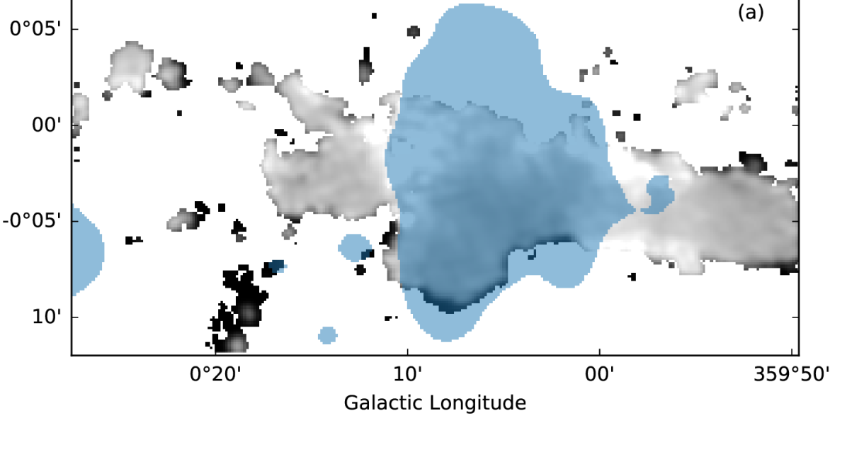
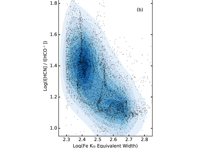
Figure 38: Data exploration of the spatial anti-correlation of EW(Fe K$\alpha$) and I(HCN)/I(HCO⁺). a) Data selection mask (blue) overlayed on a monochrome image of the I(HCN)/I(HCO⁺) ratio where darker regions indicate a lower ratio (as in the red channel in Fig. 36). The I(HCN)/I(HCO⁺) map has been smoothed to 30″ to match the resolution of the EW(Fe K$\alpha$) map. The blue mask highlights the spatial region where EW(Fe K$\alpha$)$\geq$200. b) Log-log scatter plot of EW(Fe K$\alpha$) vs. I(HCN)/I(HCO⁺) (black points) from the regions highlighted in (a) where EW(Fe K$\alpha$)$\geq$200. Blue contours represent the Gaussian kernel density estimation of the data points which highlights the overall data trend: an anti-correlation between EW(Fe K$\alpha$) and I(HCN)/I(HCO⁺).

In order to further demonstrate the effect, we have used the data exploration program Glue (Beaumont et al., 2014, 2015) to make a linked comparison between the EW(Fe K$\alpha$) and I(HCN)/I(HCO⁺) maps. To faciliate this comparison, we smoothed the integrated intensity ratio map to a 30″ Gaussian beam. This corresponds approximately to the resolution of the EW(Fe K$\alpha$) map which has variable resolution due to adaptive smoothing (Yusef-Zadeh et al., 2007). We then spatially rebinned the map I(HCN)/I(HCO⁺) to 8″ to match the EW(Fe K$\alpha$) map. Fig. 38 shows the comparison of EW(Fe K$\alpha$) and I(HCN)/I(HCO⁺). We used Glue to select the spatial region where EW(Fe K$\alpha$)$\geq$200 (blue); the spatial domain plot (Fig. 38a) displays the I(HCN)/I(HCO⁺) as a grayscale monochrome image masked (blue) by the regions where EW(Fe K$\alpha$)$\geq$200, which corresponds roughly to the region bounded by the nonthermal radiation in Fig. 36. The scatter plot (Fig. 38b) shows the pixel values of EW(Fe K$\alpha$) vs. I(HCN)/I(HCO⁺) from the masked region (black points) and a Gaussian kernel density estimation of the data points shown in blue contours. With this technique, the anti-correlation of EW(Fe K$\alpha$) and I(HCN)/I(HCO⁺) within the areas of EW(Fe K$\alpha$) $\gtrsim$ 200 and roughly bounded by the nonthermal sources is apparent. The anti-correlation does not appear to be linear (note the axes are log scale). Outside the region bounded by nonthermal sources (EW(Fe K$\alpha$) $\lesssim$ 200), there is no correlation between these quantities.

One possible interpretation is that the decreased intensity ratio traces a decreased abundance ratio. Chemical modelling by Yusef-Zadeh et al. (2013a) suggest that an increase in the cosmic ray ionization rate results in a decrease to the [HCN/HCO⁺] abundance ratio. In this scenario, the gas velocity dispersion increases due to heating of gas and damping of MHD waves by cosmic ray electrons (Yusef-Zadeh et al., 2013a). We suggest an increased cosmic ray ionization rate due to the nearby nonthermal sources may explain these observations. Multi-transition molecular line data are needed to determine the abundance ratio and test chemical models of the interaction of cosmic rays and molecular gas.

4 Summary

There have been numerous large-scale, low-resolution molecular line observations of the Galactic Center using single-dish telescopes over the last three decades. Here, we showed the first spectral line images of six different molecular species covering the inner 90$\times 50$ pc of the Galactic Center region by combining interferometric (CARMA) and single-dish (Mopra) data. This work, which also includes 3 mm continuum survey, is expected to be useful for future multi-transition studies of SiO, HCO⁺, HCN, N₂H⁺ and CS. The continuum data provided 3 mm counterpart to a number of thermal, nonthermal and IRDCs found toward the Galactic Center region. We qualititavely focussed on one aspect of the molecular line data and argued that the molecular line ratios of HCO⁺(J=1-0) and HCN(J=1-0) in the region near the Radio Arc $l\sim 0.2^{\circ}$ and the molecular gas velocity dispersion are anti-correlated with the presence of enhanced Fe K$\alpha$ line at 6.4 keV as well as 74 MHz emission. These measurements are consistent with the interaction of molecular gas with low-energy cosmic ray electrons implying that the cosmic ray ionization rate must be higher in this region of the Galaxy. The high velocity dispersion of molecular gas could be explained by the higher fraction of cosmic ray electrons coupling the magnetic field and the gas, thus increasing the damping time scale of the disturbed interacting region.

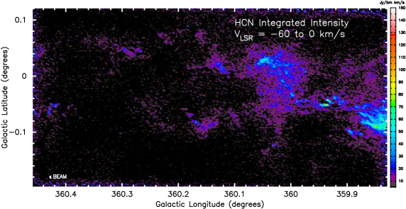
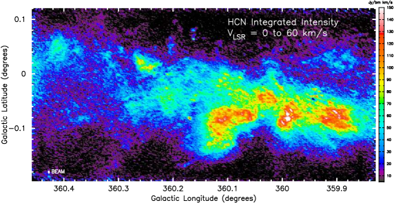
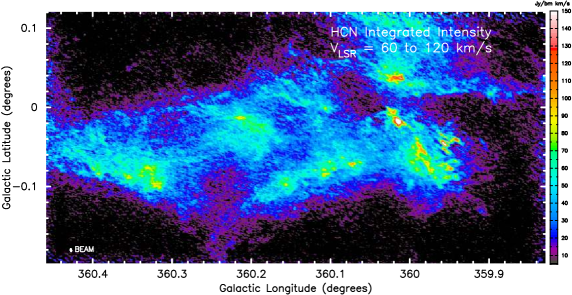
Figure 24: HCN(J=1-0) integrated intensity of the CARMA-15 plus Mopra data. Panels show integrals over selected velocity intervals: top) V_LSR= –60 to 0 ${\rm km~{}s^{-1}}$; middle) V_LSR= 0 to 60 ${\rm km~{}s^{-1}}$; bottom) V_LSR= 60 to 120 ${\rm km~{}s^{-1}}$. The color wedge indicates map intensity values.

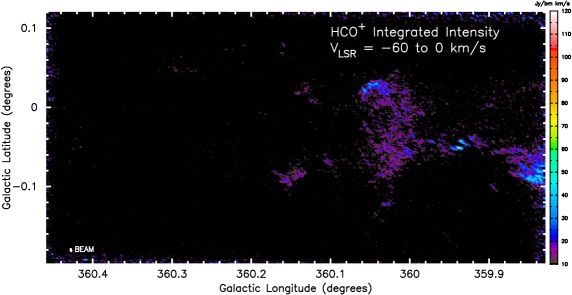
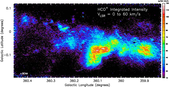
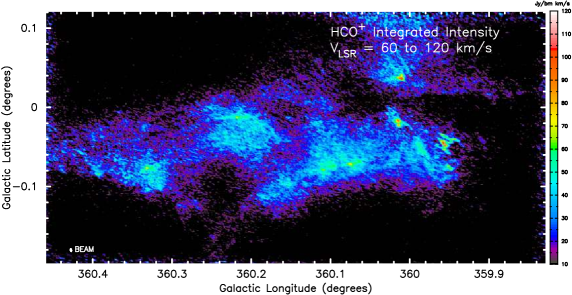
Figure 25: HCO⁺(J=1-0) integrated intensity of the CARMA-15 plus Mopra data. Panels show integrals over selected velocity intervals: top) V_LSR= –60 to 0 ${\rm km~{}s^{-1}}$; middle) V_LSR= 0 to 60 ${\rm km~{}s^{-1}}$; bottom) V_LSR= 60 to 120 ${\rm km~{}s^{-1}}$. The color wedge indicates map intensity values.

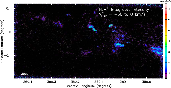
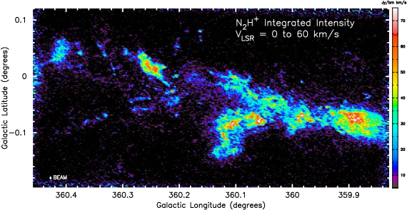
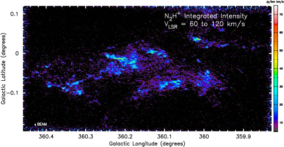
Figure 26: N₂H⁺(J=1-0) integrated intensity of the CARMA-15 plus Mopra data. Panels show integrals over selected velocity intervals: top) V_LSR= –60 to 0 ${\rm km~{}s^{-1}}$; middle) V_LSR= 0 to 60 ${\rm km~{}s^{-1}}$; bottom) V_LSR= 60 to 120 ${\rm km~{}s^{-1}}$. The color wedge indicates map intensity values.

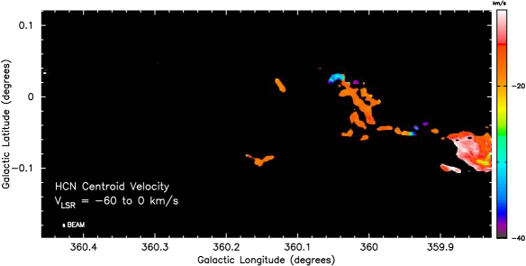
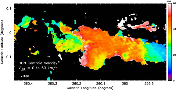
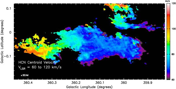
Figure 28: HCN(J=1-0) centroid velocity of the CARMA-15 plus Mopra data. Panels show integrals over selected velocity intervals: top) V_LSR= -60 to 0 ${\rm km~{}s^{-1}}$; middle) V_LSR= 0 to 60 ${\rm km~{}s^{-1}}$; bottom) V_LSR= 60 to 120 ${\rm km~{}s^{-1}}$; and the color wedge indicates map centroid velocity values.

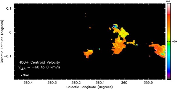
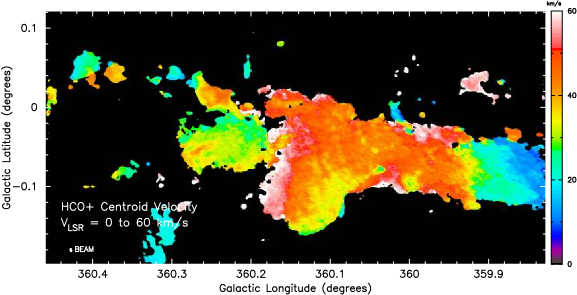
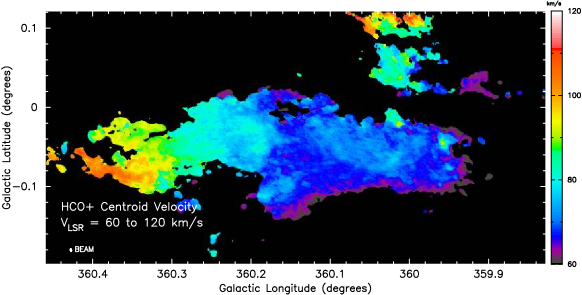
Figure 29: HCO⁺(J=1-0) centroid velocity of the CARMA-15 plus Mopra data. Panels show integrals over selected velocity intervals: top) V_LSR= -60 to 0 ${\rm km~{}s^{-1}}$; middle) V_LSR= 0 to 60 ${\rm km~{}s^{-1}}$; bottom) V_LSR= 60 to 120 ${\rm km~{}s^{-1}}$; and the color wedge indicates map centroid velocity values;

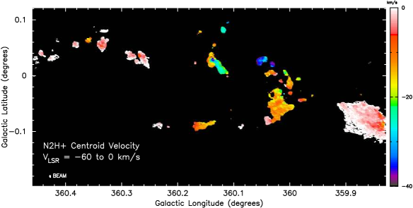
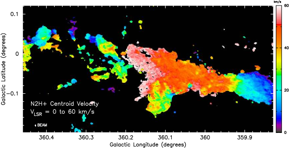
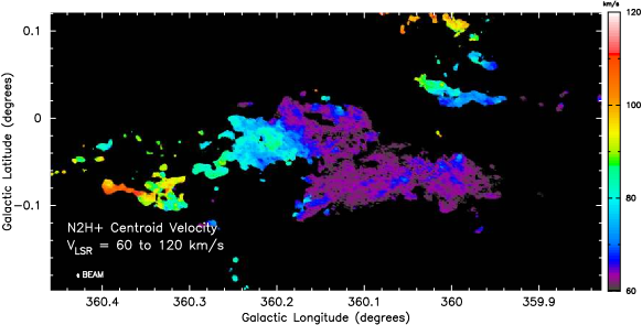
Figure 30: N₂H⁺(J=1-0) centroid velocity of the CARMA-15 plus Mopra data. Panels show integrals over selected velocity intervals: top) V_LSR= -60 to 0 ${\rm km~{}s^{-1}}$; middle) V_LSR= 0 to 60 ${\rm km~{}s^{-1}}$; bottom) V_LSR= 60 to 120 ${\rm km~{}s^{-1}}$; and the color wedge indicates map centroid velocity values.

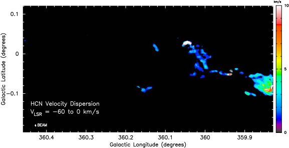
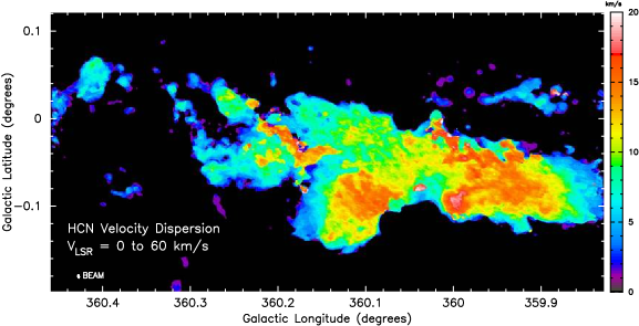
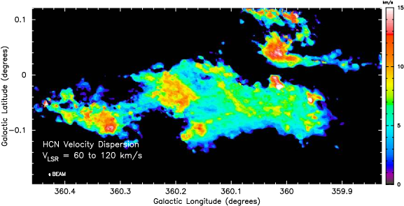
Figure 32: HCN(J=1-0) one-dimensional velocity dispersion of the CARMA-15 plus Mopra data. Panels show integrals over selected velocity intervals: top) V_LSR= -60 to 0 ${\rm km~{}s^{-1}}$; middle) V_LSR= 0 to 60 ${\rm km~{}s^{-1}}$; bottom) V_LSR= 60 to 120 ${\rm km~{}s^{-1}}$; and the color wedge indicates map velocity dispersion values.

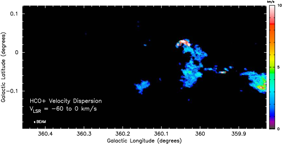
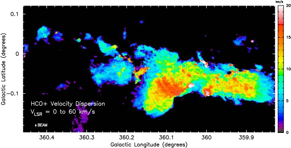
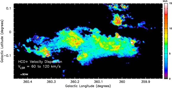
Figure 33: HCO⁺(J=1-0) one-dimensional velocity dispersion of the CARMA-15 plus Mopra data. Panels show integrals over selected velocity intervals: top) V_LSR= -60 to 0 ${\rm km~{}s^{-1}}$; middle) V_LSR= 0 to 60 ${\rm km~{}s^{-1}}$; bottom) V_LSR= 60 to 120 ${\rm km~{}s^{-1}}$; and color wedge indicates map velocity dispersion values.

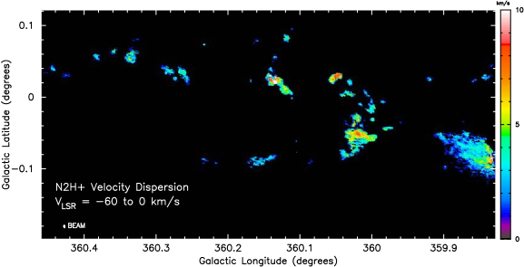
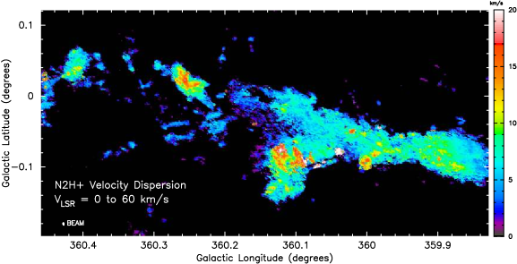
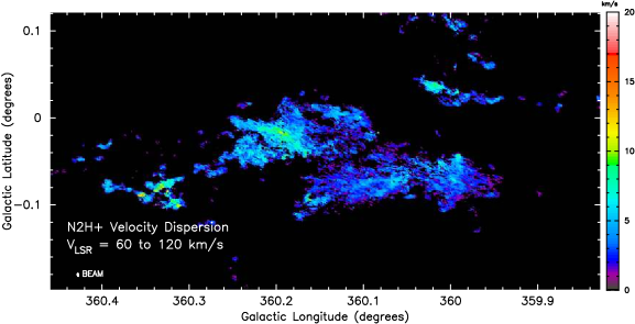
Figure 34: N₂H⁺(J=1-0) one-dimensional velocity dispersion of the CARMA-15 plus Mopra data. Panels show integrals over selected velocity intervals: top) V_LSR= -60 to 0 ${\rm km~{}s^{-1}}$; middle) V_LSR= 0 to 60 ${\rm km~{}s^{-1}}$; bottom) V_LSR= 60 to 120 ${\rm km~{}s^{-1}}$; and color wedge indicates map velocity dispersion values.

References

- Anderson et al. (2011) Anderson L. D., Bania T. M., Balser D. S., Rood R. T., 2011, ApJS, 194, 32
- Archer et al. (2016) Archer A., et al., 2016, ApJ, 821, 129
- Argon et al. (2000) Argon A. L., Reid M. J., Menten K. M., 2000, ApJS, 129, 159
- Beaumont et al. (2014) Beaumont C., Robitaille T., Borkin M., 2014, Glue: Linked data visualizations across multiple files, Astrophysics Source Code Library (ascl:1402.002)
- Beaumont et al. (2015) Beaumont C., Goodman A., Greenfield P., 2015, in Taylor A. R., Rosolowsky E., eds, Astronomical Society of the Pacific Conference Series Vol. 495, Astronomical Data Analysis Software an Systems XXIV (ADASS XXIV). p. 101
- Becker et al. (1994) Becker R. H., White R. L., Helfand D. J., Zoonematkermani S., 1994, ApJS, 91, 347
- Bock et al. (2006) Bock D. C.-J., et al., 2006, in Society of Photo-Optical Instrumentation Engineers (SPIE) Conference Series. p. 626713, doi:10.1117/12.674051
- Briggs (1995) Briggs D. S., 1995, in American Astronomical Society Meeting Abstracts. p. 1444
- Brogan et al. (2003) Brogan C. L., Nord M., Kassim N., Lazio J., Anantharamaiah K., 2003, Astronomische Nachrichten Supplement, 324, 17
- Brown (1987) Brown R. L., 1987, in Dalgarno A., Layzer D., eds, Spectroscopy of Astrophysical Plasmas. pp 35–58
- Caswell et al. (1995) Caswell J. L., Vaile R. A., Ellingsen S. P., Whiteoak J. B., Norris R. P., 1995, MNRAS, 272, 96
- Cotton & Yusef-Zadeh (2016) Cotton W. D., Yusef-Zadeh F., 2016, ApJS, 227, 10
- Coutens et al. (2017) Coutens A., Rawlings J. M. C., Viti S., Williams D. A., 2017, MNRAS, 467, 737
- Di Francesco et al. (2008) Di Francesco J., Johnstone D., Kirk H., MacKenzie T., Ledwosinska E., 2008, ApJS, 175, 277
- Ekers et al. (1983) Ekers R. D., van Gorkom J. H., Schwarz U. J., Goss W. M., 1983, A&A, 122, 143
- Felli et al. (2002) Felli M., Testi L., Schuller F., Omont A., 2002, A&A, 392, 971
- Goto et al. (2014) Goto M., Geballe T. R., Indriolo N., Yusef-Zadeh F., Usuda T., Henning T., Oka T., 2014, ApJ, 786, 96
- HESS Collaboration et al. (2016) HESS Collaboration et al., 2016, Nature, 531, 476
- Helfer et al. (2003) Helfer T. T., Thornley M. D., Regan M. W., Wong T., Sheth K., Vogel S. N., Blitz L., Bock D. C.-J., 2003, ApJS, 145, 259
- Hill et al. (2005) Hill T., Burton M. G., Minier V., Thompson M. A., Walsh A. J., Hunt-Cunningham M., Garay G., 2005, MNRAS, 363, 405
- Ho et al. (1985) Ho P. T. P., Jackson J. M., Barrett A. H., Armstrong J. T., 1985, ApJ, 288, 575
- Immer et al. (2012) Immer K., Schuller F., Omont A., Menten K. M., 2012, A&A, 537, A121
- Johnston et al. (2014) Johnston K. G., Beuther H., Linz H., Schmiedeke A., Ragan S. E., Henning T., 2014, A&A, 568, A56
- Jones et al. (2012) Jones P. A., et al., 2012, MNRAS, 419, 2961
- Jones et al. (2013) Jones P. A., Burton M. G., Cunningham M. R., Tothill N. F. H., Walsh A. J., 2013, MNRAS, 433, 221
- Kauffmann et al. (2013) Kauffmann J., Pillai T., Zhang Q., 2013, ApJ, 765, L35
- Koyama et al. (1996) Koyama K., Maeda Y., Sonobe T., Takeshima T., Tanaka Y., Yamauchi S., 1996, PASJ, 48, 249
- LaRosa et al. (2000) LaRosa T. N., Kassim N. E., Lazio T. J. W., Hyman S. D., 2000, AJ, 119, 207
- LaRosa et al. (2005) LaRosa T. N., Brogan C. L., Shore S. N., Lazio T. J., Kassim N. E., Nord M. E., 2005, ApJ, 626, L23
- Lang et al. (1999) Lang C. C., Morris M., Echevarria L., 1999, ApJ, 526, 727
- Lang et al. (2010) Lang C. C., Goss W. M., Cyganowski C., Clubb K. I., 2010, ApJS, 191, 275
- Lazio & Cordes (2008) Lazio T. J. W., Cordes J. M., 2008, ApJS, 174, 481
- Le Petit et al. (2016) Le Petit F., Ruaud M., Bron E., Godard B., Roueff E., Languignon D., Le Bourlot J., 2016, A&A, 585, A105
- Lis & Carlstrom (1994) Lis D. C., Carlstrom J. E., 1994, ApJ, 424, 189
- Lis et al. (2001) Lis D. C., Serabyn E., Zylka R., Li Y., 2001, ApJ, 550, 761
- Longmore et al. (2012) Longmore S. N., et al., 2012, ApJ, 746, 117
- Ludovici et al. (2016) Ludovici D. A., Lang C. C., Morris M. R., Mutel R., Mills E. A. C., Toomey IV J. E., Ott J., 2016, ApJ, 826, 218
- Mills et al. (2011) Mills E., Morris M. R., Lang C. C., Dong H., Wang Q. D., Cotera A., Stolovy S. R., 2011, ApJ, 735, 84
- Mills et al. (2015) Mills E. A. C., Butterfield N., Ludovici D. A., Lang C. C., Ott J., Morris M. R., Schmitz S., 2015, ApJ, 805, 72
- Molinari et al. (2011) Molinari S., et al., 2011, ApJ, 735, L33
- Muno et al. (2006) Muno M. P., Bauer F. E., Bandyopadhyay R. M., Wang Q. D., 2006, ApJS, 165, 173
- Murakami et al. (2000) Murakami H., Koyama K., Sakano M., Tsujimoto M., Maeda Y., 2000, ApJ, 534, 283
- Murakami et al. (2001) Murakami H., Koyama K., Maeda Y., 2001, ApJ, 558, 687
- Nord et al. (2004) Nord M. E., Lazio T. J. W., Kassim N. E., Hyman S. D., LaRosa T. N., Brogan C. L., Duric N., 2004, AJ, 128, 1646
- Oka et al. (2005) Oka T., Geballe T. R., Goto M., Usuda T., McCall B. J., 2005, ApJ, 632, 882
- Paumard et al. (2006) Paumard T., et al., 2006, ApJ, 643, 1011
- Pierce-Price et al. (2000) Pierce-Price D., et al., 2000, ApJ, 545, L121
- Ponti et al. (2010) Ponti G., Terrier R., Goldwurm A., Belanger G., Trap G., 2010, ApJ, 714, 732
- Rathborne et al. (2014) Rathborne J. M., et al., 2014, ApJ, 786, 140
- Rathborne et al. (2015) Rathborne J. M., et al., 2015, ApJ, 802, 125
- Rodríguez & Zapata (2013) Rodríguez L. F., Zapata L. A., 2013, ApJ, 767, L13
- Rosolowsky et al. (2010) Rosolowsky E., et al., 2010, ApJS, 188, 123
- Sault et al. (1995) Sault R. J., Teuben P. J., Wright M. C. H., 1995, in Shaw R. A., Payne H. E., Hayes J. J. E., eds, Astronomical Society of the Pacific Conference Series Vol. 77, Astronomical Data Analysis Software and Systems IV. p. 433 (arXiv:astro-ph/0612759)
- Soldi et al. (2014) Soldi S., Clavel M., Goldwurm A., Morris M. R., Ponti G., Terrier R., Trap G., 2014, in Sjouwerman L. O., Lang C. C., Ott J., eds, IAU Symposium Vol. 303, The Galactic Center: Feeding and Feedback in a Normal Galactic Nucleus. pp 94–96, doi:10.1017/S1743921314000258
- Steer et al. (1984) Steer D. G., Dewdney P. E., Ito M. R., 1984, A&A, 137, 159
- Storm et al. (2014) Storm S., et al., 2014, ApJ, 794, 165
- Toomey (2014) Toomey IV J., 2014, Master’s thesis, The University of Iowa
- Tsuboi et al. (2016) Tsuboi M., Kitamura Y., Miyoshi M., Uehara K., Tsutsumi T., Miyazaki A., 2016, PASJ, 68, L7
- Walsh et al. (1998) Walsh A. J., Burton M. G., Hyland A. R., Robinson G., 1998, MNRAS, 301, 640
- Walsh et al. (2003) Walsh A. J., Macdonald G. H., Alvey N. D. S., Burton M. G., Lee J.-K., 2003, A&A, 410, 597
- Walsh et al. (2011) Walsh A. J., et al., 2011, MNRAS, 416, 1764
- Wenger et al. (2000) Wenger M., et al., 2000, A&AS, 143, 9
- Wright et al. (2001) Wright M. C. H., Coil A. L., McGary R. S., Ho P. T. P., Harris A. I., 2001, ApJ, 551, 254
- Yusef-Zadeh & Morris (1987a) Yusef-Zadeh F., Morris M., 1987a, AJ, 94, 1178
- Yusef-Zadeh & Morris (1987b) Yusef-Zadeh F., Morris M., 1987b, ApJ, 320, 545
- Yusef-Zadeh et al. (1984) Yusef-Zadeh F., Morris M., Chance D., 1984, Nature, 310, 557
- Yusef-Zadeh et al. (2002) Yusef-Zadeh F., Law C., Wardle M., 2002, ApJ, 568, L121
- Yusef-Zadeh et al. (2004) Yusef-Zadeh F., Hewitt J. W., Cotton W., 2004, ApJS, 155, 421
- Yusef-Zadeh et al. (2005) Yusef-Zadeh F., Wardle M., Muno M., Law C., Pound M., 2005, Advances in Space Research, 35, 1074
- Yusef-Zadeh et al. (2007) Yusef-Zadeh F., Muno M., Wardle M., Lis D. C., 2007, ApJ, 656, 847
- Yusef-Zadeh et al. (2009) Yusef-Zadeh F., et al., 2009, ApJ, 702, 178
- Yusef-Zadeh et al. (2010) Yusef-Zadeh F., Lacy J. H., Wardle M., Whitney B., Bushouse H., Roberts D. A., Arendt R. G., 2010, ApJ, 725, 1429
- Yusef-Zadeh et al. (2013a) Yusef-Zadeh F., Wardle M., Lis D., Viti S., Brogan C., Chambers E., Pound M., Rickert M., 2013a, Journal of Physical Chemistry A, 117, 9404
- Yusef-Zadeh et al. (2013b) Yusef-Zadeh F., et al., 2013b, ApJ, 762, 33
- Zhao et al. (1993) Zhao J.-H., Desai K., Goss W. M., Yusef-Zadeh F., 1993, ApJ, 418, 235