The wiggly cosmic string as a waveguide for massless and massive fields

Abstract

We examine the effect of a wiggly cosmic string for both massless and massive particle propagation along the string axis. We show that the wave equation that governs the propagation of a scalar field in the neighborhood of a wiggly string is formally equivalent to the quantum wave equation describing the hydrogen atom in two dimensions. We further show that the wiggly string spacetime behaves as a gravitational waveguide in which the quantized wave modes propagate with frequencies that depend on the mass, string energy density, and string tension. We propose an analogy with an optical fiber, defining an effective refractive index likely to mimic the cosmic string effect in the laboratory.

I Introduction

The thermal history of the Universe started 14 billion years ago with an extremely hot and dense quark-gluon plasma that cooled down in the inflation era. As a consequence, it has undergone a succession of phase transitions involving spontaneous symmetry-breaking (SSB) mechanisms. Below an energy scale $M_{\rm GUT}\sim 10^{16}$ GeV, the strong forces are represented by the three-fold color symmetry, associated with the gauge group $SU(3)_{\rm color}$, whereas the weak and electromagnetic forces are mixed into the electroweak interaction, represented by weak isospin symmetry (gauge group $SU(2)_{\rm L}$) and hypercharge symmetry (gauge group $U(1)_{\rm Y}$) Weinberg (1995). This is the realm of the particle physics standard model, which has been tested to a very high precision. Above $M_{\rm GUT}$, strong and electroweak interactions unify within a larger gauge symmetry group G where grand unified theories involving supersymmetry (SUSY GUT) have been considered as suitable description for such energy scales Bajc et al. (2004); Fukuyama et al. (2005); Raby (2011).

As well-known in condensed matter physics (CMP), spontaneoulsy symmetry breaking (SSB) lead to phase transitions which often give rise to the appearance of topological defects. Interestingly, a mechanism originally proposed by Kibble Kibble (1976) to describe the birth and dynamics of a network of defects in a cosmological context revealed to be relevant in the condensed matter realm, for example in liquid crystals. Bowick et al. (1994). To determine what kind of topological defect emerges for a given SSB transition $G\rightarrow H$, one may study the content of homotopy groups $\pi_{k}(G/H)$ of the vacuum manifold $\mathcal{M}=G/H$ Kenna (2006). If $\pi_{k}(G/H)\neq 0$, defects of dimension $2-k$ are formed: for $k=0$, defects are 2D (grain boundaries in CMP, domain walls in cosmology), for $k=1$, defects are line-like (disclinations or dislocations in CMP, cosmic strings in cosmology) and for $k=2$, defects are point-like (e.g. hedgehogs in CMP, monopoles in cosmology…).

Even though the SUSY extension to the standard model still has to pass experimental verification (the first run of the LHC found no evidence for supersymmetry), it provides a route to the formation of cosmic strings. In a seminal paper, Jeannerot et al Jeannerot et al. (2003) examined all possible SSB patterns from the large possible SUSY GUT gauge groups down to the standard model $SU(3)_{\rm color}\times SU(2)_{\rm L}\times U(1)_{\rm Y}$ and concluded that cosmic string formation was unavoidable. Another possibility for cosmic string generation is brane inflation Dvali and Tye (1999). Cosmic strings, seen as lower-dimensional D-branes which are one-dimensional in the noncompact directions, may have been abundantly produced by brane collision towards the end of the brane inflationary period Sarangi and Tye (2002).

Despite all theoretical justifications for the existence of cosmic strings, the observational evidence is still feeble and mostly indirect. Nevertheless, the search for cosmic strings is very active and it happens in such diverse fronts as the cosmic microwave background Hergt et al. (2017) and gravitational wave bursts Stott et al. (2017). As warned by Copeland and Kibble Copeland and Kibble (2010), “Both cosmic strings and superstrings are still purely hypothetical objects. There is no direct empirical evidence for their existence, though there have been some intriguing observations that were initially thought to provide such evidence, but are now generally believed to have been false alarms. Nevertheless, there are good theoretical reasons for believing that these exotic objects do exist, and reasonable prospects of detecting their existence within the next few years.”

In this paper, we study the dynamics of particles in the vicinity of a wiggly cosmic string. Regular straight strings are linear defects for which the geometry is globally that of a cone and therefore, spacetime is locally flat, except on string axis. Indeed, for such objects, the line tension $T_{0}$ exactly matches the energy density per unit length $\mu_{0}$, such that straight strings do not gravitate. Recent data on the Cosmic Microwave Background collected from PLANCK satellite have not confirmed the existence of these objects yet, but they have set upper boundaries on their mass-energy density Ade and al. (2014) $G\mu_{0}<10^{-7}$ ($c=1$). Refined models for cosmic strings may involve small-scale perturbations such as kinks and wiggles Vilenkin and Shellard (1994). The presence of wiggles generates a far gravitational field contribution which may be responsible for an elliptical distortion of the shape of background galaxies Dyda and Brandenberger (2007); Feng (2012) or for the accretion of dark energy around the defectGonzalez-Diaz and Jiménez Madrid (2006). Averaging the effect of these perturbations along a string increases the linear mass density $\tilde{\mu}$ and decreases the string tension $\tilde{T}$, respecting the equation of state Carter (1990); Vilenkin (1990)$\tilde{\mu}\>\tilde{T}=\mu_{0}^{2}$, leading the wiggly string to exert a gravitational pulling on neighboring objects. In the weak-field approximation, the linearized line element representing the spacetime of a wiggly string oriented along the $z$-axis is given byVachaspati and Vilenkin (1991); Vilenkin and Shellard (1994):

$$ds^{2} = -\left(1+8\varepsilon\ln\left({r}/{r_{0}}\right)\right)dt^{2}+dr^{2}+\alpha^{2}r^{2}d\theta^{2}$$ (1)

$$+ \left(1-8\varepsilon\ln\left({r}/{r_{0}}\right)\right)dz^{2}.$$

Here, $\alpha^{2}=1-4G(\tilde{\mu}+\tilde{T})$, where $4G(\tilde{\mu}+\tilde{T})\ll 1$ meaning that conical deficit angle $4G\pi(\tilde{\mu}+\tilde{T})$ associated to the string is very small. The parameter $\varepsilon$ is defined as the excess of mass-energy density, $2\varepsilon=G(\tilde{\mu}-\tilde{T})$. It must be emphasized that $G(\tilde{\mu}+\tilde{T})$ and $\varepsilon$ are two independent parameters: the former accounts for the discrepancy between flat and conical geometries, whereas the latter accounts for the discrepancy between straight and wiggly strings. The constant $r_{0}$ denotes the effective string radius Peter (1994). In the remainder of this work, propagation of particles will be considered only within the region $r_{0}<r\ll r_{0}e^{1/{8\varepsilon}}$, in order to avoid the logarithmic divergence at small and large distances from the defect. Hence, $h_{00}=8\varepsilon\ln\left({r}/{r_{0}}\right)=O(\varepsilon)\ll 1$.

In the next sections of this work, the wave equation for propagation along the string axis is numerically solved in the background spacetime given by metric (1). The properties of the radially bound states and the dispersion relations are examined in detail for both massless and massive particles. Then an analogy with light propagation in an optical fiber is performed to design a system likely to mimic the effect of a cosmic wiggly string in laboratory.

II Massless particle propagation

In a plane perpendicular to the wiggly string, light propagates in the same way as in the vicinity of a regular straight string Vilenkin and Shellard (1994), that is without experiencing any gravitational force. On the contrary, when the direction of propagation is not perpendicular to the string, the wiggly string exerts gravitational pulling on light passing by, as the background spacetime is not locally Euclidean. Consequently, the wave equation governing propagation of a scalar field in this background geometry needs to account for its curvature. This is done by using the 4-dimensional Laplace-Beltrami operator in the wave equation

$$\frac{1}{\sqrt{-g}}\partial_{\mu}(\sqrt{-g}g^{\mu\nu}\partial_{\nu})\Phi=0,$$ (2)

where $\Phi=\Phi(r,\theta,z,t)$ is the scalar wave amplitude and $g=\det(g_{\mu\nu})$ with the metric tensor $g_{\mu\nu}$ coming from metric (1). In terms of the metric (1), this gives

$$-(1-h_{00})\partial_{t}^{2}\Phi+\frac{1}{r}\partial_{r}\left(r\partial_{r}\right)\Phi+\frac{1}{\alpha^{2}r^{2}}\partial_{\theta}^{2}\Phi$$

$$\qquad\qquad+(1+h_{00})\partial_{z}^{2}\Phi=0.$$ (3)

As the field is single-valued, $\Phi$ has to be periodic in $\theta$:

$$\Phi(\theta)=\Phi(\theta+2\pi).$$ (4)

To solve equation (3) we make the ansatz

$$\Phi(r,\theta,z,t)=e^{il\theta}e^{i(\omega t-kz)}R(r),$$ (5)

where the wave vector $k\in\mathbb{R}$, $l=0,\pm 1,\pm 2...$ specifies the angular momentum and $\omega$ is an angular frequency. Substituting the general solution (5) into equation (3), we get

$$-\frac{1}{r}\frac{d}{dr}\left(r\frac{dR}{dr}\right) +\frac{l^{2}}{\alpha^{2}r^{2}}R+h_{00}\left(\omega^{2}+k^{2}\right)R$$ (6)

$$=\left(\omega^{2}-k^{2}\right)R.$$

Defining the dimensionless variables $\rho=r/\gamma$, $\rho_{0}=r_{0}/\gamma$, where $\gamma=\left[8\varepsilon\left(\omega^{2}+k^{2}\right)\right]^{-1/2}$, then multiplying (6) by $\gamma^{2}\sim O(\varepsilon^{-1})$ and rearranging terms gives the eigenvalue equation:

$$-\frac{1}{\rho}\frac{d}{d\rho}\left(\rho\frac{dR}{d\rho}\right) + \left(\frac{{l}^{2}}{\alpha^{2}\rho^{2}}+\ln{\frac{\rho}{\rho_{0}}}\right)R=\bar{\zeta}R$$ (7)

with

$$\bar{\zeta}=\frac{1}{8\varepsilon}\frac{\omega^{2}-k^{2}}{\omega^{2}+k^{2}}.$$ (8)

We note that the potential behaving logarithmically, the energy scale cannot be fixed at infinity and we work in the following with $\omega-$dependent length units such that $\rho_{0}=1$. Eq. (7) is formally equivalent to the Schrödinger equation that describes the hydrogen atom in the 2D Coulomb potential. Hence, the potential term in Eq. (7), $V_{\rm eff}=\frac{{l}^{2}}{\alpha^{2}\rho^{2}}+\ln{\frac{\rho}{\rho_{0}}}$ (see figure 1) only accommodates for bound states Asturias and Aragon (1985); Eveker et al. (1990); Garon et al. (2013).

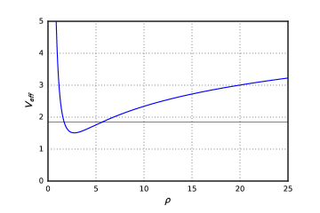
Figure 1: Effective potential, $V_{\rm eff}$ (in units where $\rho_{0}=1$), for $l=2$. The horizontal solid line represents the ground state $\bar{\zeta}$ at that value of $l$.

As a consequence, in the geometrical optics limit, trajectories are radially bounded helices around the string, as appears in Fig. 2, explicitly showing the gravitational pulling by the string. This is in agreement with Ref. Arazi and Simeone, 2000, where geodesics near a Brans-Dicke wiggly cosmic string were also found to be bounded. The minimum and maximum radii are solutions of the transcendental equation $\bar{\zeta}=V_{\rm eff}$ whereas the pitch is given by the ratio between the angular and effective linear momenta ${\frac{l}{k}}$. In the case of $l=0$ the trajectory is rectilinear and parallel to the string.

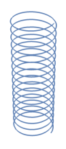
(a) ref1

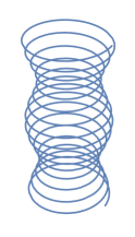
(b) ref2

Figure 2: Possible ray paths corresponding to the geometric optics limit of a scalar wave propagating along the wiggly string: (a) when the “total energy” $\bar{\zeta}$ is at the minimum of the effective potential and (b) at some point above it.

In order to solve equation (7), we used a finite difference method Van der Maelen Uría et al. (1996); Franklin and Garon (2011); Burden and Faires (2011) and computed numerically the radial part of the waves traveling along the wiggly string with their corresponding eigenvalues. The different states are labeled by quantum numbers $n$ (radial quantum number) and $l$. In Fig. 3, we plot the lowest three eigenvalues $\bar{\zeta_{nl}}$ of the wave equation (7) and the corresponding radial wave amplitudes $R_{nl}(\rho)$ for $l=0,\pm 1,\pm 2$.

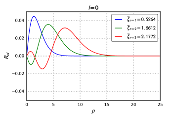
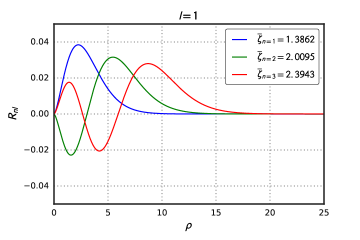
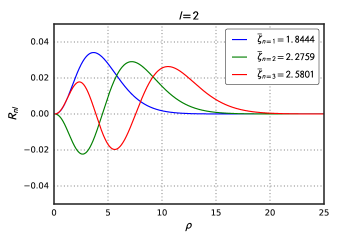
Figure 3: Wave modes for the first lowest eigenvalues $n=1,2,3$ of Eq. (7) for each $l=0,1,2$.

From Eq. (8) we see that the wave modes that propagate along the wiggly string axis are quantized by $n$ and $l$. It has been suggested that cosmic structures with a non-vanishing Newtonian potential could generally behave as gravitational waveguide for light and massive particles Dodonov and Man’ko (1989); Bimonte et al. (1998) and we examine this proposition in the following. The dispersion relation is given by:

$$\omega^{2}_{nl}=\frac{1}{n^{2}_{1}}k^{2}$$ (9)

where

$$n_{1}=\left[\frac{1-8\varepsilon\bar{\mathcal{\zeta}_{nl}}}{1+8\varepsilon\bar{\mathcal{\zeta}_{nl}}}\right]^{1/2}$$ (10)

is an effective refractive index. From Eq. (9) we see that modes are propagative along the string provided that the following requirement is fulfilled:

$$0<\bar{\zeta}_{nl}<\frac{1}{4G(\tilde{\mu}-\tilde{T})}.$$ (11)

This constraint establishes that the number of wave modes propagating along the wiggly string is large but finite as in an ordinary electromagnetic waveguide. As we would expect, we find that the allowed modes, besides being quantized by $n$ and $l$, their frequency also depend on both the energy density and the tension of the string.

III Propagation of Massive Particles

Since light propagating along a wiggly string is radially confined, as seen in the previous section, it is interesting to investigate what happens to massive particles under the same circumstances. In order to study this possibility we write the Klein-Gordon equation ($\hbar=1$) in the wiggly string background geometry:

$$\left[\frac{1}{\sqrt{-g}}\partial_{\mu}(\sqrt{-g}g^{\mu\nu}\partial_{\nu})-m^{2}\right]\Phi(r,\theta,z,t)=0,$$ (12)

where now $\Phi$ is a complex scalar field describing spinless relativistic particles. Using the ansatz given in Eq. (5) in equation (12), and following the same procedures used above in the case of massless particles propagation, we arrive to an identical eigenvalue equation as (7), but with eigenvalues given by

$$\bar{\mathcal{E}}_{nl}=\frac{1}{8\varepsilon}\frac{{\omega^{2}}-k^{2}-m^{2}}{{\omega^{2}}+k^{2}},$$ (13)

thus the wavefunctions $R_{nl}(\rho)$ and the eigenvalues $\bar{\mathcal{E}}_{nl}$ are numerically identical to the solution of the equation (7) (see figure (3)). In addition, the discussion on the geometric optics limit of the propagating massless field is still valid for massive particles. However, inclusion of the mass term in the dispersion relation now introduces a cutoff:

$$\omega_{nl}^{2}=\frac{1}{n^{2}_{2}}k^{2}+\omega_{c}^{2}$$ (14)

where $n_{2}$ is an effective refractive index defined by

$$n_{2}=\left[\frac{1-8\varepsilon\bar{\mathcal{E}}_{nl}}{1+8\varepsilon\bar{\mathcal{E}}_{nl}}\right]^{1/2},$$ (15)

which has an identical generic form than $n_{1}$, and

$$\omega_{c}^{2}=\frac{m^{2}}{1-8\varepsilon\mathcal{E}_{nl}}$$ (16)

is a cutoff frequency.

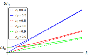
Figure 4: The angular frequency $\omega_{nl}$ in terms of the wavelength $k$ for different values of $n_{1}$ and $n_{2}$. While the dashed lines corresponding to massless particles are obviously linear and the solid lines which correspond to the massive case have a quadratic start, both cases are fixed by mode-dependent parameters.

The dispersion relation (14) presents a forbidden band as it occurs for electromagnetic waves propagating in an unmagnetized plasma Jackson (1999). The wave will propagate along the string when its frequency is larger than the cutoff frequency, $\omega_{c}$, otherwise solutions appear as evanescent waves. At high frequencies, $\omega\gg\omega_{c}$, we recover the massless dispersion relation (9). Moreover, the constraint

$$0<\bar{\mathcal{E}_{nl}}<\frac{1}{4G(\tilde{\mu}-\tilde{T})},$$ (17)

like in the massless case, sets a limit to a finite number of propagating modes. Besides the dependence on the density of energy and tension of the wiggly string, the allowed propagating modes also depend on the mass of the particle.

There is obviously a strong similarity between the propagation of both massless and massive scalar fields along a wiggly cosmic string and the propagation of electromagnetic waves in optical waveguides. In the next section, we further explore this analogy by proposing a way of designing an optical fiber that mimics the wiggly string in the context described above.

IV Analogue Optical Waveguide

The analogy between 3D gravity and optics is an old topic that started with the pioneering works of Gordon on Fresnel dragging effect in moving dielectrics Gordon (1923). Recently, artificial optical materials (metamaterials) have been proposed as a way to mimic aspects of curved spacetime in the laboratory. For instance, by manipulating the effective refractive index of the medium, Sheng et al. Sheng et al. (2013) were able to reproduce gravitational lensing and trapping of light (see also Genov et al. (2009)). Incidentally, electronic metamaterials may also be used to simulate peculiar spacetime conditions, like a discontinuous Lorentzian to Kleinian metric signature change Figueiredo et al. (2016) which has also been modeled by optical metamaterials Smolyaninov and Narimanov (2010). Liquid crystals, as well, have been used to simulate straight cosmic strings Sátiro and Moraes (2006) and the Schwarzschild spacetime Pereira and Moraes (2011). On the other hand, it has been proposed that, by spatially varying the doping concentration, the refractive index profile of optical fibers can be used to control optical transmission in a designer-specified way de Lima Bernardo and Moraes (2011). Following this standpoint, we investigate the proposition of a graded-index optical fiber that reproduces some of the properties of the scalar field propagation along a wiggly string.

In general, the wave equations for electromagnetic waves propagating along a circular fiber are coupled Jackson (1999). This implies that there is no separation into purely TE or TM modes but, in the specific case of a fiber with an azimuthally symmetric refractive index, if the fields have no dependence on the azimuthal angle, the equations uncouple into separate scalar wave equations of the form

$$\left[\frac{1}{r}\frac{\partial}{\partial r}\left(r\frac{\partial}{\partial r}\right)+\frac{\partial^{2}}{\partial z^{2}}+n^{2}(r)\omega^{2}\right]\Phi=0,$$ (18)

where $\omega$ is the angular frequency, $n(r)$ is the optical fiber refractive index and $\operatorname{Re}\left({\Phi}\right)$ represents any real component of the field. For waves propagating along the optical fiber ($z$-direction), the ansatz $\Phi(r,z)=e^{-ikz}R(r)$, (where $k\in\mathbb{R}$) substituted into Eq. (18) gives

$$-\frac{1}{r}\frac{d}{dr}\left(r\frac{dR}{dr}\right)-n^{2}(r)\omega^{2}R+k^{2}R=0.$$ (19)

Here, we choose the refractive index to be given by

$$n(r)=\left(1-\Omega\ln{\frac{r}{r_{0}}}\right)^{1/2},$$ (20)

with the dimensionless parameter $\Omega\ll 1$ in order to be consistent with the wiggly string parameter $\varepsilon$. The quantity $r_{0}$ is considered to be much smaller than the radius $r_{f}$ of the fiber and defines an opaque core radius. This way, by considering propagation in the region $r_{0}<r<r_{f}$, the logarithmic singularity at $r=0$ is avoided. Like in the previous sections, we change $r$ to dimensionless units by doing the change of variables $\rho=r/\nu$, $\rho_{0}=r_{0}/\nu$ and setting $\nu=\Omega^{-1/2}\omega^{-1}$. Then, the dimensionless equation for the optical fiber can be written as:

$$-\frac{1}{\rho}\frac{d}{d\rho}\left(\rho\frac{dR}{d\rho}\right)+\left(\ln{\frac{\rho}{\rho_{0}}}\right)R=\bar{\beta}_{n}R,$$ (21)

where

$$\bar{\beta}_{n}=\frac{1}{\Omega}\left({1-\frac{k^{2}}{\omega^{2}}}\right).$$ (22)

The radial amplitudes of the wave and their corresponding eigenvalues in the optical fiber with the refractive index given by Eq. (20) obey equations identical to the ones of massless and massive particles propagating with $l=0$ in the spacetime of a wiggly string. For a given $z$, the intensity profiles for the propagating waves described by Eq. (7) are given by $2\pi\rho R_{nl}^{2}(\rho)$. In Fig. 5, we plot the intensity distribution for different wave modes, solutions of Eq. (7). The optical fiber modes described by Eq. (21) correspond to the cases where $l=0$.

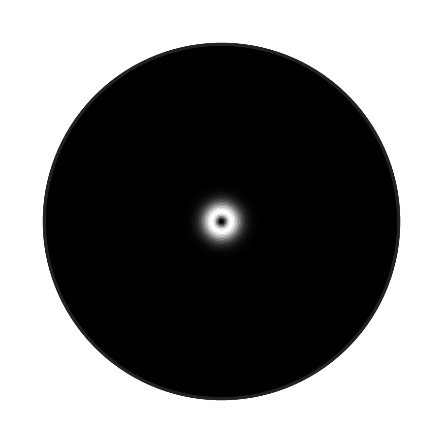
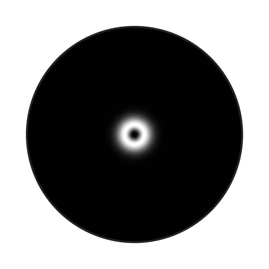
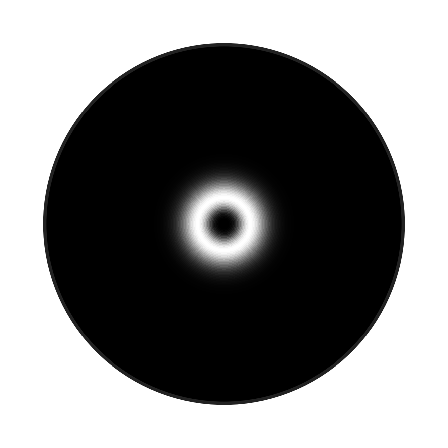
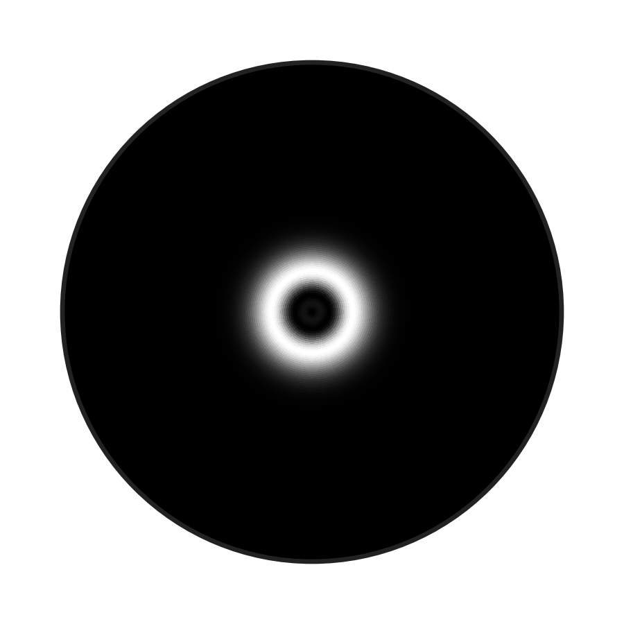
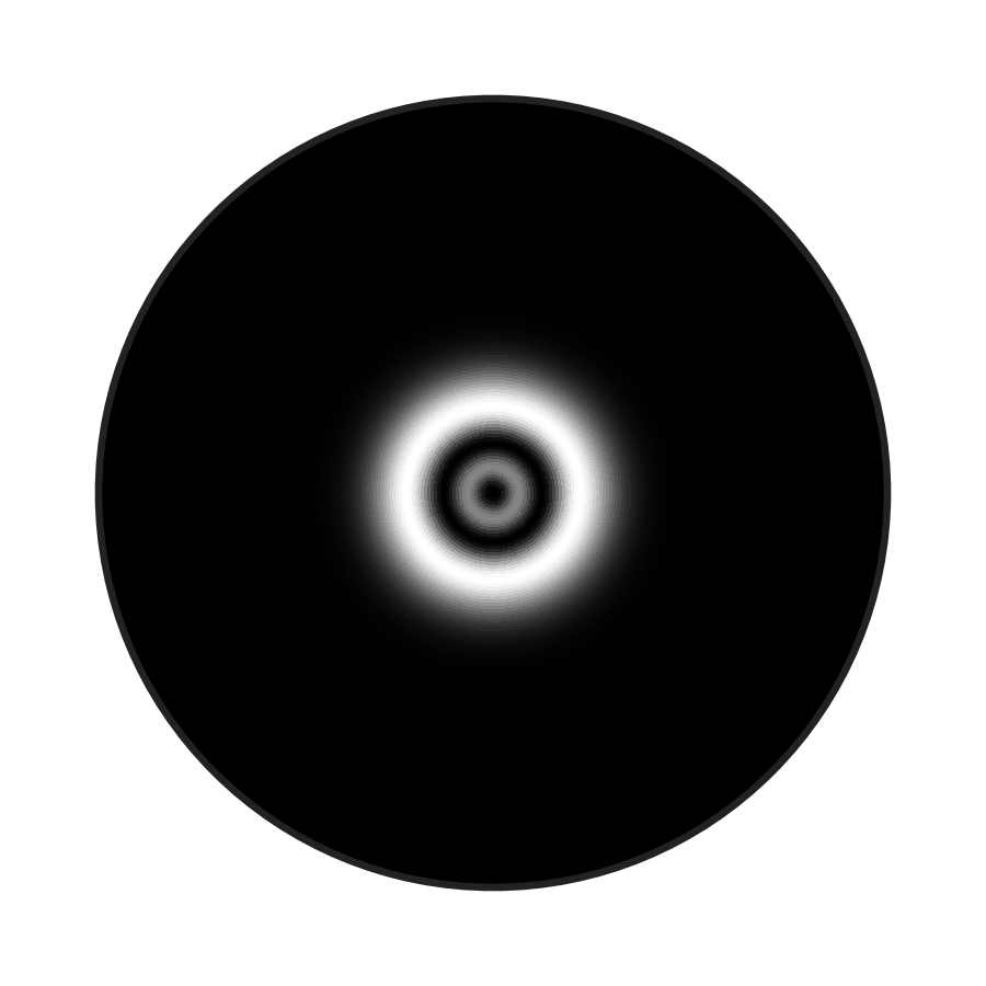
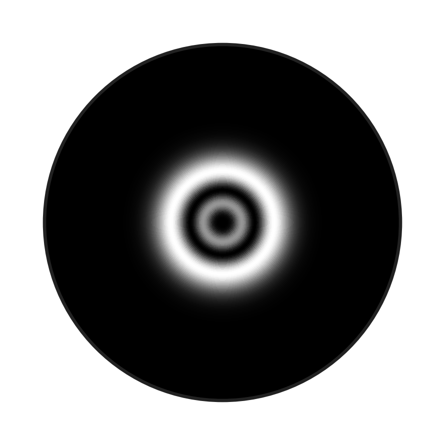
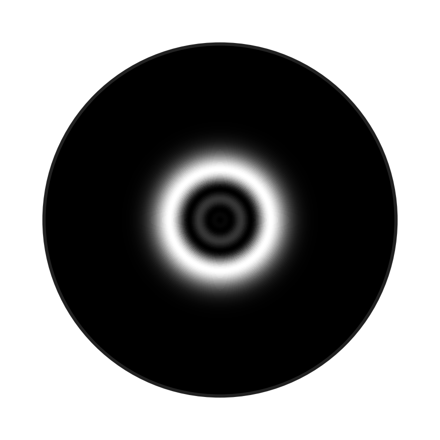
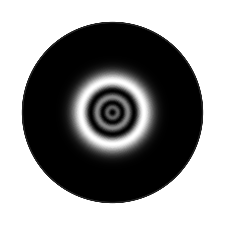
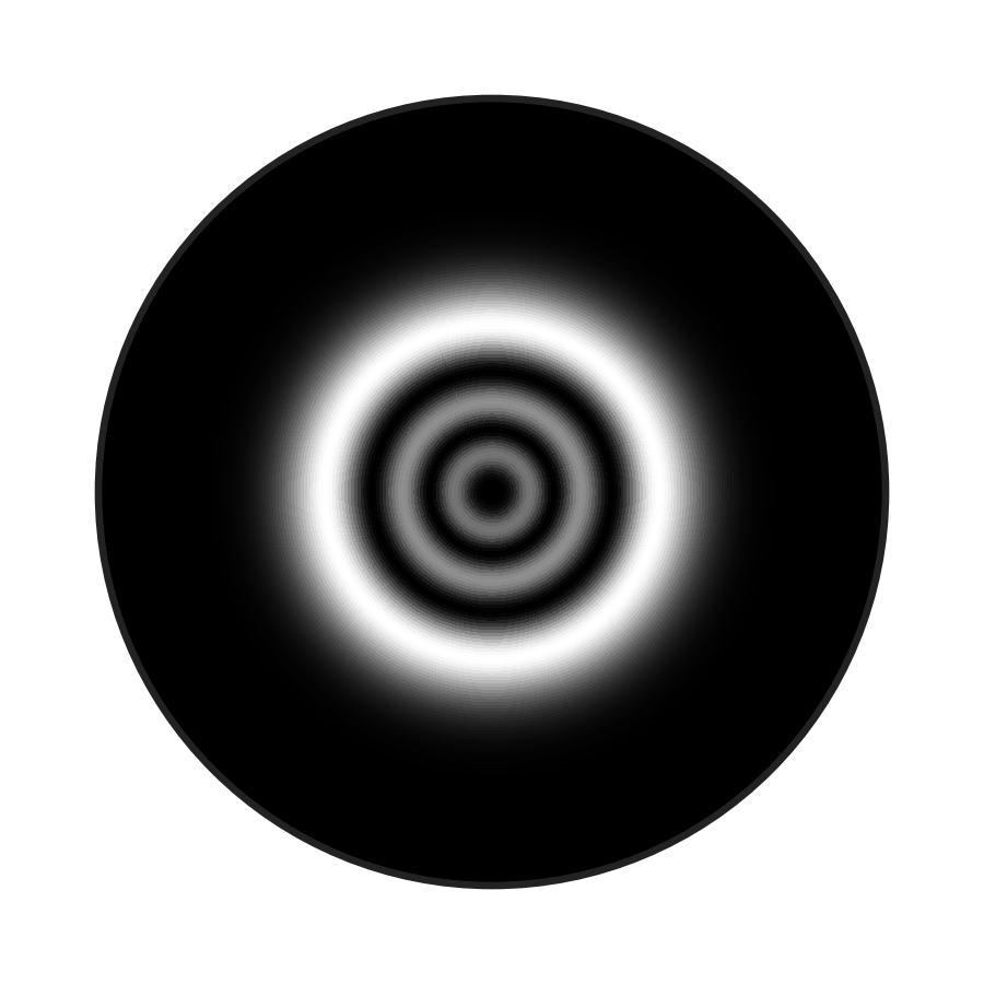
Figure 5: Intensity profiles for the first few solutions $R_{nl}^{2}$ of Eq. (7), with $n=1,2,3$ and $l=0,1,2$. The profiles are disposed as in a matrix where $n$ and $l$ give the line and column number, respectively. The first column corresponds to the optical fiber modes described by Eq. (21).

Before ending this section, we remark that the coupled equations for the electromagnetic field in the circular optical fiber, in the more general case where the field depends on the azimuthal angle but the refractive index remains azimuthally symmetric, give rise to hybrid HE modes (no longer TE or TM) Jackson (1999). The case of a step-index fiber was studied in Ref. Snitzer (1961) which found the field to be of the form $R_{l}(\rho)e^{il\theta}$, where $R_{l}$ is a Bessel function. Even though Eq. (7) is not a Bessel equation, its symmetries and the shape of the numerical solutions shown in Fig. 3, suggest that a solution in terms of an expansion on Bessel functions might be rapidly convergent. The $\theta$-dependence of the scalar fields solutions, for $l\neq 0$, is therefore reminiscent of what happens in the circular optical fiber. Also, it would be interesting to compare the coupled electromagnetic vector field equations for a wave propagating along a circular optical fiber with refractive index given by Eq. (20) with the electromagnetic field equations in the wiggly string background.

V Conclusion

In this paper, we examined the effect of wiggly cosmic strings on propagation of massless and massive fields. We found that waves propagating along the string axis experience the small-scale perturbations which make the propagation qualitatively different from that of waves propagating in the background spacetime with a unperturbed cosmic string. The non-vanishing Newtonian potential acts as an inhomogeneous dielectric medium so that the massless particles are radially confined in a vicinity of the defect axis. Therefore, the wiggly string spacetime behaves as a gravitational waveguide in which wave modes are quantized. These latter depend on the string energy density and string tension. The number of allowed modes is finite as in a ordinary optical waveguides. On the other hand, the presence of wiggles cause gravitational pullings on massive objects, making the waveguide effect to be also valid for massive fields propagation. In this case, the frequencies of the waves also depend on the mass of the particle.

Finally, we proposed the design of an optical fiber with a non homogeneous refractive index profile likely to mimic the effect of a perturbed cosmic string. The radial solutions with the corresponding eigenvalues were found by using a numerical method. Although we have considered here the propagation of massive and massless scalar fields along a wiggly string, the extension to vector fields like vector bosons or the electromagnetic field can be of interest. In particular, as a perspective for future work we mention the study of propagating electromagnetic waves along the wiggly string and a possible correspondence with an optical fiber. This is more complex than the problem presented here since the vector field equations are coupled and cannot be reduced to scalar wave equations.

Another aspect of of the optical fiber/wiggly string analogy is whether a propagating electromagnetic wave along the wiggly string could act as a tractor field on particles in the string vicinity. This has been proposed recently in the realm of negative index optical waveguides Salandrino and Christodoulides (2011): instead of being pushed by radiative pressure, a polarizable particle in such environment is attracted by the source of radiation. Even though the requirement of a negative refractive index rules out the wiggly string as such waveguide, a related linear defect, the hyperbolic disclination Fumeron et al. (2015), seems to be a plausible mediator of this effect. The Kleinian signature of its metric simulates a negative refractive index.

Networks of cosmic topological defects have been proposed as models for solid dark matter Bucher and Spergel (1999). This suggests that one might explore the optical implications of a network of wiggly strings. For instance, for a periodic array of strings one might expect some of the properties of a photonic crystal, like the appearance of band gaps in the dispersion relation, which limit the propagation to the allowed regions of the spectrum. This is presently under investigation and will be the subject of a future publication.