The flat bottomed lines of Vega

R.Monier LESIA, UMR 8109, Observatoire de Paris Meudon, Place J.Janssen, Meudon, France M.Gebran Department of Physics and Astronomy, Notre Dame University - Louaize, PO Box 72, Zouk Mikael, Lebanon F.Royer GEPI,UMR 8111, Observatoire de Paris Meudon, Place J.Janssen, Meudon, France T. Kılıcoğlu Department of Astronomy and Space Sciences, Faculty of Science, Ankara University, 06100, Ankara, Turkey

Abstract

Using one high dispersion high quality spectrum of Vega (HR7001, A0V) obtained with the échelle spectrograph SOPHIE at Observatoire de Haute Provence, we have measured the centroids of 149 flat-bottomed lines. The model atmosphere and spectrum synthesis modeling of the spectrum of Vega allows us to provide identifications for all these lines. Most of these lines are due to C I, O I, Mg I, Al I, Ca I, Sc II,Ti II, Cr I, Cr II, Mn I, Fe I, Fe II, Sr II, Ba II, the large majority being due to neutral species, in particular Fe I.

keywords:

stars: individual, stars: Vega, HR 7001

1 Introduction

Vega (HR 7001), the standard A0V spectral type, is one of the 47 northern slowly rotating early-A stars studied by Royer et al. (2014). The low projected rotational velocity of HR 7001, about 24 ${\mathrm{km~{}s^{-1}}}$ is due to the very low inclination angle ( $i\simeq 0$ ) while the equatorial velocity $v_{e}\simeq 245{\mathrm{km~{}s^{-1}}}$ is very large (Gulliver et al. 1994). Hence Vega is a fast rotator seen nearly pole-on whose limb almost coincides with the equator of the star. At the equator, the centrifugal forece reduces the effective surface gravity which alters the ionization balance and strengthens the local $I_{\lambda}$ profile of certain species. For these species, the distribution of the Doppler shift is bimodal, ie. arises from the two equatorial regions near the limb. We have measured all the centroids of all 149 flat-bottomed lines we could find in the high resolution SOPHIE spectrum of Vega. We have synthesized all lines expected to be present in the SOPHIE spectrum of HR 7001 in the range 3900 up to 6800 Å using model atmospheres and spectrum synthesis and an appropriate chemical composition for Vega as derived by Castelli & Kurucz (1994). The synthetic spectrum has been adjusted adjusted to the SOPHIE spectrum of HR 7001 in order to identify the flat-bottomed lines of HR 7001

2 Observations and reduction

A search of the SOPHIE archive reveals that HR 7001 has been observed 78 times at the Observatoire de Haute Provence using SOPHIE from 03 August 2006 to 06 August 2012. We have used one high resolution (R = 75000) 30 seconds exposure secured with a $\frac{S}{N}$ ratio of about 824 at 5000 Å to search for the flat-bottomed lines.

3 Model atmospheres and spectrum synthesis

The effective temperature and surface gravity of HR 7001 were first evaluated using Napiwotzky et al’s (1993) UVBYBETA calibration of Stromgren’s photometry. The found effective temperature ${\mathrm{T_{eff}}}$ is 9550 $\pm$ 200 K and the surface gravity ${\mathrm{\log g}}$ is $3.98\pm$ 0.25 dex. This temperature is in very good agreement with the fundamental temperature derived by Code et al. (1976) from the integrated flux and the angular diameter and with the mean temperature and surface gravity derived by Hill et al. (2010).

A plane parallel model atmosphere assuming radiative equilibrium, hydrostatic equilibrium and local thermodynamical equilibrium was then computed using the ATLAS9 code (Kurucz 1992), specifically the linux version using the new ODFs maintained by F. Castelli on her website^*^**http://www.oact.inaf.it/castelli/. The linelist was built starting from Kurucz’s (1992) gfhyperall.dat file ^†^††http://kurucz.harvard.edu/linelists/ which includes hyperfine splitting levels. This first linelist was then upgraded using the NIST Atomic Spectra Database ^‡^‡‡http://physics.nist.gov/cgi-bin/AtData/linesform and the VALD database operated at Uppsala University (Kupka et al. 2000)^§^§§http://vald.astro.uu.se/ vald/php/vald.php. A grid of synthetic spectra was then computed with a modified version of SYNSPEC49 (Hubeny & Lanz 1992, 1995) to model the lines. The synthetic spectrum was then convolved with a gaussian instrumental profile and a parabolic rotation profile using the routine ROTIN3 provided along with SYNSPEC49. We adopted a projected apparent rotational velocity $v_{e}\sin i=24.5$ km.s^-1 and a radial velocity $v_{rad}=-13.80$ km.s^-1 from Royer et al. (2014).

4 Determination of the microturbulent velocity

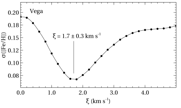
In order to derive the microturbulent velocity of HR 7001, we have derived the iron abundance [Fe/H] by using 36 unblended Fe II lines for a set of microturbulent velocities ranging from 0.0 to 2.5 ${\mathrm{km~{}s^{-1}}}$ . Figure 1 shows the standard deviation of the derived [Fe/H] as a function of the microturbulent velocity. The adopted microturbulent velocity is the value which minimizes the standard deviation ie. for that value, all Fe II lines yield the same iron abundance, which is [Fe/H] = -0.60 $\pm$ 0.07 dex. Hence iron is found to be underabundant in HR 7001 in agreement with previous abundance determinations (Castelli & Kurucz 1994). We therefore adopt a microturbulent velocity $\xi_{t}$ = 1.70 $\pm$ 0.04 ${\mathrm{km~{}s^{-1}}}$ constant with depth for HR 7001.

Refer to caption — Figure 1: The derived microturbulent velocity for HR 7001

5 The list of flat-bottomed lines in HR 7001

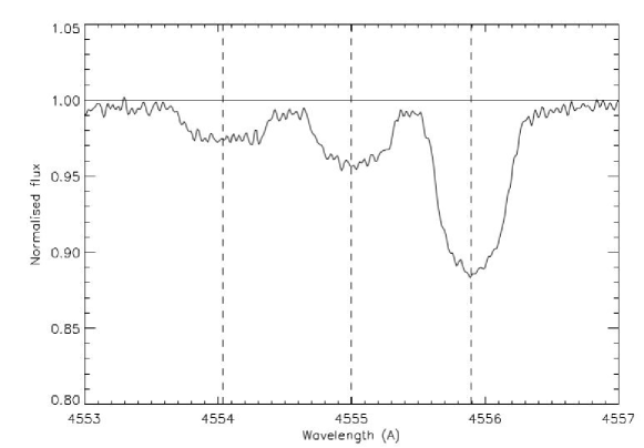
An example of flat-bottomed line in the spectrum of HR 7001 is the Ba II line at 4554.04 Å shown in Fig. 2. Note that the lines of Cr II at 4554.99 Å and of Fe II at 4555.99 Å have normal profiles. All the flat-bottomed lines are collected together with their identifications in Tab. LABEL:longtab-atom. These lines are weak lines due to C I, O I, Mg I, Al I, Ca I, Sc II, Ti II, Cr I, Cr II, Mn I, Fe I, Fe II, Sr II, Ba II, the large majority being due to neutral species, in particular Fe I. Most of the lines we find to be flat-bottomed are also listed in the investigation of weak lines conducted by Takeda et al. (2008) in their high signal-to-noise high resolution spectrum of Vega.

6 Conclusions

A systematic search for flat-bottomed lines in the high resolution high quality SOPHIE spectrum of HR 7001 yields 149 lines in the range 3900 Å up to 6800 Å which complete the previous list published by Takeda et al. (2008). Most of these lines are due to C I, O I, Mg I, Al I, Ca I, Sc II,Ti II, Cr I, Cr II, Mn I, Fe I, Fe II, Sr II, Ba II, the large majority being due to Fe I.

Table 1: Identifications for flat-bottomed lines in Vega

$\lambda_{\mathrm{obs}}$ (Å)	$\lambda_{\mathrm{lab}}$ (Å)	Species	$\log gf$	$E_{low}$	Comments
3903.08	3902.945	Fe I	-0.47	12560.933
3916.45	3916.45	V II	-1.060	11514.760
3918.64	3918.642	Fe I	-0.720	24338.766
3920.31	3920.258	Fe I	-1.75	978.074
3922.94	3922.912	Fe I	-1.65	415.933
3927.98	3927.920	Fe I	-1.59	888.132
3930.31	3930.296	Fe I	-1.590	704.007
	3930.304	Fe II	-4.030	13673.186
3932.06	3932.023	Ti II	-1.780	9118.260
3935.98	3935.962	Fe II	-1.860	44915.046
3938.32	3938.289	Fe II	-3.890	13474.411
	3938.400	Mg I	-0.760	35051.263
3944.03	3944.006	Al I	-0.620	0.000
3945.20	3945.210	Fe II	-4.250	13673.186
3956.71	3956.677	Fe I	-0.430	21715.731
3961.54	3961.520	Al I	-0.320	112.061
4002.36	4002.483	Cr II	-2.060	42897.990	?
4005.29	4005.242	Fe I	-0.610	12560.933
4021.88	4021.866	Fe I	-0.660	22249.428
4034.49	4034.469	Mn I	-0.810	0.000
	4034.502	Mn I	-0.810	0.000
4035.67	4035.595	Fe I	-1.100	34039.315	blend
	4035.627	V II	-0.960	14461.750
	4035.694	Mn I	-0.190	17281.999
	4035.713	Mn I	-0.190	17281.999
	4035.715	Mn I	-0.190	17281.999
4043.99	4043.897	Fe I	-0.830	26140.178	blend
	4043.977	Fe I	-1.130	26140.178
	4044.012	Fe II	-2.410	44929.549
4057.56	4057.461	Fe II	-1.550	58668.256	blend
	4057.505	Mg I	-1.200	35031.263
4068.01	4067.978	Fe I	-0.430	25899.986
4070.89	4070.840	Cr II	-0.750	52321.010
4072.38	4072.502	Fe I	-1.440	27666.345
4118.57	4118.545	Fe I	0.280	28819.952
4122.69	4122.668	Fe II	-3.380	20830.553
4132.11	4132.058	Fe I	-0.650	12968.554
4134.67	4134.677	Fe I	-0.490	22838.320
4143.37	4143.415	Fe I	-0.200	24574.652
4143.86	4143.868	Fe I	-0.450	12560.933
4161.58	4161.535	Ti II	-2.360	8744.250
4167.34	4167.271	Mg I	-1.600	35051.263	blend
	4167.299	Fe II	-0.560	90300.626
4175.69	4175.036	Fe I	-0.670	22946.815
4176.63	4176.566	Fe I	-0.620	27166.817
4181.74	4181.755	Fe I	-0.180	22838.320
4187.06	4187.039	Fe I	-0.550	19757.031
4187.83	4187.795	Fe I	-0.550	19562.437
4191.49	4191.430	Fe I	-0.670	19912.494
4198.29	4198.247	Fe I	-0.460	27166.817	blend
	4198.304	Fe I	-0.720	19350.891
4199.11	4199.095	Fe I	0.250	24574.655
4202.02	4202.029	Fe I	-0.710	11976.238
4210.40	4210.343	Fe I	-0.870	20019.633
	4210.383	Fe I	-1.240	24772.016
4215.60	4215.519	Sr II	-0.140	0.000
4219.40	4219.360	Fe I	0.120	28819.952
4222.30	4222.213	Fe I	-0.970	19757.031	blend
	4222.381	Zr II	-0.900	9742.800
4226.75	4226.728	Ca I	0.240	0.000
4227.45	4227.427	Fe I	0.230	26874.546
4236.00	4235.936	Fe I	-0.340	19562.437
4238.80	4238.810	Fe I	-0.280	27394.689	blend
	4238.819	Fe II	-2.720	54902.315
4250.15	4250.119	Fe I	-0.410	19912.494
4250.80	4250.787	Fe I	-0.710	12560.933
4273.30	4273.326	Fe II	-3.260	21812.055
4274.80	4274.797	Cr I	-0.230	0.000
4275.60	4275.606	Cr II	-1.710	31117.390
4278.20	4278.159	Fe II	-3.820	21711.917
4282.45	4282.403	Fe I	-0.810	17550.180	blend
	4282.490	Mn II	-1.680	44521.521
4284.20	4284.188	Cr II	-1.860	31082.940
4287.90	4287.872	Ti II	-2.020	8710.440
4312.90	4312.864	Ti II	-1.160	9518.060
4325.0	4324.999	Sc II	-0.440	4802.870
4367.6	4367.659	Ti II	-1.270	20891.660	blend
	4367.578	Fe I	-1.270	24118.816
4369.50	4369.411	Fe II	-3.670	22469.852
4371.4	4371.367	C I	-2.330	61981.822
4386.9	4386.844	Ti II	-1.260	20951.600
4394.05	4394.051	Ti II	-1.590	9850.900
4395.08	4395.033	Ti II	-0.660	8744.250
4400.40	4400.379	Sc II	-0.510	4883.570
4411.10	4411.074	Ti II	-1.060	24561.031
4417.80	4417.719	Ti II	-1.430	9395.710
4418.40	4418.330	Ti II	-2.460	9975.920
4450.60	4450.482	Ti II	-1.450	8744.250
4451.60	4451.551	Fe II	-1.840	49506.995
4454.90	4455.027	Fe I	-1.090	31307.244
4464.50	4464.450	Ti II	-2.080	9363.620
4466.65	4466.551	Fe I	-0.590	22856.320
4473.00	4472.929	Fe II	-3.430	22939.357
4476.10	4476.019	Fe I	-0.570	22946.815	blend
	4476.076	Fe I	-0.290	29732.735
4488.40	4488.331	Ti II	-0.820	25192.791
4494.65	4494.563	Fe I	-1.140	17726.928
4528.70	4528.614	Fe I	-0.820	17550.180
4529.60	4529.569	Fe II	-3.190	44929.549
4541.60	4541.524	Fe II	-3.050	23031.299
4554.20	4554.033	Ba II		0.000	15 hfs iso
4582.85	4582.835	Fe II	-3.100	22939.357
4590.0	4589.958	Ti II	-1.790	9975.920	blend
	4589.967	O I	-2.390	86631.153
4592.10	4592.049	Cr II	-1.220	32854.949
4616.60	4616.629	Cr II	-1.290	32844.760
4620.50	4620.521	Fe II	-3.280	22810.356
4666.80	4666.758	Fe II	-3.330	22810.356
4703.00	4702.991	Mg I	-0.670	35051.263	blend
	4702.991	Zr II	-0.800	20080.301
4731.50	4731.453	Fe II	-3.360	23317.632
4736.82	4736.773	Fe I	-0.740	25899.986	very weak
4775.90	4775.897	C I	-2.670	18145.285
4780.00	4779.985	Ti II	-1.370	16518.860
4812.40	4812.468	Fe I	-5.400	22249.428
4836.20	4836.229	Cr II	-2.250	31117.390
4890.70	4890.755	Fe I	-0.430	23192.497
4891.50	4891.492	Fe I	-0.140	22996.673	blend
	4891.485	Cr II	-3.040	31350.901
4919.05	4918.994	Fe I	-0.370	23110.937	blend
	4918.954	Fe I	-0.340	33507.120
4920.50	4920.502	Fe I	0.060	22845.868
4932.00	4932.049	C I	-1.880	61981.822	blend
	4932.080	Fe II	-1.730	83196.488
4934.10	4934.076	Ba II	-0.150	0.000
4993.40	4993.565	N I	-2.860	95475.313	?
5004.20	5004.195	Fe II	0.500	82853.660
5052.20	5052.167	C I	-1.650	61981.822	very flat bottomed
5129.20	5129.152	Ti II	-1.390	15257.430
5133.70	5133.688	Fe I	0.140	33695.394
5154.00	5154.070	Ti II	-1.920	12628.731
5171.60	5171.596	Fe I	-1.790	11976.238	blend, very extended flat core
	5171.640	Fe II	-4.370	22637.205
5185.90	5185.913	Ti II	-1.350	15265.619
5188.70	5188.680	Ti II	-1.210	12758.110
5192.40	5192.442	Fe II	-2.020	5192.442
5206.00	5206.037	Cr I	0.020	7593.150
5208.40	5208.425	Cr I	0.160	7593.150
5217.00	5216.863	Fe II	0.610	84527.779	blend
	5216.854	Fe II	0.390	84710.686
5226.60	5226.343	Ti II	-1.300	12628.731
5226.84	5226.862	Fe I	-0.550	24506.914
5227.30	5227.481	Fe II	0.800	84296.829	blend
	5227.323	Fe II	-0.030	84344.832
5237.40	5237.329	Cr II	-1.150	32854.311
5255.00	5254.929	Fe II	-3.230	26055.422
5266.60	5266.555	Fe I	-0.490	24180.861
5269.60	5269.537	Fe I	-1.320	6928.268
5275.01	5274.964	Cr II	-1.29	32836.680
5291.65	5291.666	Fe II	0.58	84527.779
5313.55	5313.563	Cr II	-1.650	32854.949
5324.20	5324.179	Fe I	-0.240	25899.986
5325.50	5325.503	Fe II	-2.800	25981.670
5329.70	5329.673	O I	-2.200	86627.777	blend
	5329.681	O I	-1.610	86627.777
	5329.690	O I	-1.410	86627.777
5330.80	5330.726	O I	-2.570	86631.453	blend
	5330.735	O I	-1.710	86631.453
	5330.741	O I	-1.120	86631.453
5336.80	5336.771	Ti II	-1.700	12758.110
5337.60	5337.732	Fe II	- 3.890	26055.422
	5337.772	Cr II	-2.030	32854.949
5362.92	5362.869	Fe II	-2.740	25805.329	blend
	5362.957	Fe II	-0.080	84685.798
5367.50	5367.466	Fe I	0.350	35611.622
5370.00	5369.961	Fe I	0.350	35257.323	blend
	5370.164	Cr II	0.320	86782.011
5371.50	5371.489	Fe I	-1.650	7728.059	blend
	5371.437	Fe I	-1.240	35767.561
5380.35	5380.337	C I	-1.840	97770.180
5383.30	5383.369	Fe I	0.500	34782.420
5404.15	5404.117	Fe I	0.540	34782.420	blend
	5404.151	Fe I	0.520	35767.561
5405.80	5405.663	Fe II	-0.440	48708.863	blend
	5405.775	Fe I	-1.840	7985.784
5410.90	5410.910	Fe I	0.280	36079.371
5415.20	5415.199	Fe I	0.500	35379.205
5425.20	5425.257	Fe II	-3.360	25805.329
5447.00	5446.916	Fe I	-1.930	7985.784
5455.50	5455.454	Fe I	0.300	34843.934	blend
	5455.609	Fe I	-2.090	8154.713
5526.80	5526.770	Sc II	0.130	14261.320
5528.40	5528.405	Mg I	-0.620	35051.263
5534.80	5534.847	Fe II	-2.940	26170.181	blend
	5534.890	Fe II	-0.690	85048.620
5572.75	5572.842	Fe II	-0.310	27394.689
5586.80	5586.842	Cr II	0.910	88001.361	blend
	5586.756	Fe I	-0.210	27166.817
5588.70	5588.619	Cr II	-5.550	31117.390
5615.70	5615.644	Fe I	-0.140	26874.547
5669.0	5668.943	C I	-2.430	68856.328	blend
	5669.038	Sc II	-1.120	12101.499
6147.70	6147.741	Fe II	-2.720	31364.440
6149.30	6149.258	Fe II	-2.720	31968.450
6162.0	6162.173	Ca I	0.100	15315.943	very weak
6238.35	6238.392	Fe II	-2.630	31364.440
6247.45	6247.557	Fe II	-2.330	31307.949
6417.00	6416.919	Fe II	-2.740	31387.949

Acknowledgements.

The authors acknowledge use of the SOPHIE archive (http://atlas.obs-hp.fr/sophie/) at Observatoire de Haute Provence. They have used the NIST Atomic Spectra Database and the VALD database operated at Uppsala University (Kupka et al., 2000) to upgrade atomic data.

References

Castelli & Kurucz (1994) Castelli, F., Kurucz, R.L. 1994, A&A, 281, 817
Code et al. (1976) Code, A., D., Davis, J., Bless, R.C., Hanbury Brown, R. 1976, ApJ, 203, 417
Gulliver et al. (1994) Gulliver, A.F., Hill, G., Adelman, S.J. 1994, ApJ, 429L, 81G
Hill et al. (2010) Hill, G., Gulliver, A.F., Adelman, S.J. 2010, ApJ, 712, 250
Hubeny & Lanz (1992) Hubeny, I., Lanz, T. 1992, A&A, 262, 501
Hubeny & Lanz (1995) Hubeny, I., Lanz, T. 1995, ApJ, 439, 875
Kupka et al. (2000) Kupka F., Ryabchikova T.A., Piskunov N.E., Stempels H.C., Weiss W.W., 2000, Baltic Astronomy, vol. 9, 590-594
Kurucz (1992) Kurucz, R.L. 1992, Rev. Mexicana. Astron. Astrofis., 23, 45
Napiwotzki et al. (1993) Napiwotzki, R., Schoenberner, D., Wenske, V. 1993, A&A, 268, 653
Royer et al. (2014) Royer, F., Gebran, M., Monier, R., Adelman, S., Smalley, B., Pintado, O., Reiners, A., Hill, G., Gulliver, G. 2014 , A&A, 562A, 84R
Takeda et al. (2008) Takeda, Y., Kawanomoto, S., Ohishi, N. 2008, ApJ, 678, 446