Replicability Analysis for Natural Language Processing: Testing Significance with Multiple Datasets
Abstract
With the ever growing amounts of textual data from a large variety of languages, domains and genres, it has become standard to evaluate NLP algorithms on multiple datasets in order to ensure consistent performance across heterogeneous setups. However, such multiple comparisons pose significant challenges to traditional statistical analysis methods in NLP and can lead to erroneous conclusions. In this paper we propose a Replicability Analysis framework for a statistically sound analysis of multiple comparisons between algorithms for NLP tasks. We discuss the theoretical advantages of this framework over the current, statistically unjustified, practice in the NLP literature, and demonstrate its empirical value across four applications: multi-domain dependency parsing, multilingual POS tagging, cross-domain sentiment classification and word similarity prediction. 111Our code is at: https://github.com/rtmdrr/replicability-analysis-NLP .
1 Introduction
The field of Natural Language Processing (NLP) is going through the data revolution. With the persistent increase of the heterogeneous web, for the first time in human history, written language from multiple languages, domains, and genres is now abundant. Naturally, the expectations from NLP algorithms also grow and evaluating a new algorithm on as many languages, domains, and genres as possible is becoming a de-facto standard.
For example, the phrase structure parsers of ?) and ?) were mostly evaluated on the Wall Street Journal Penn Treebank [Marcus et al. (1993], consisting of written, edited English text of economic news. In contrast, modern dependency parsers are expected to excel on the 19 languages of the CoNLL 2006-2007 shared tasks on multilingual dependency parsing [Buchholz and Marsi (2006, Nilsson et al. (2007], and additional challenges, such as the shared task on parsing multiple English Web domains [Petrov and McDonald (2012], are continuously proposed.
Despite the growing number of evaluation tasks, the analysis toolbox employed by NLP researchers has remained quite stable. Indeed, in most experimental NLP papers, several algorithms are compared on a number of datasets where the performance of each algorithm is reported together with per-dataset statistical significance figures. However, with the growing number of evaluation datasets, it becomes more challenging to draw comprehensive conclusions from such comparisons. This is because although the probability of drawing an erroneous conclusion from a single comparison is small, with multiple comparisons the probability of making one or more false claims may be very high.
The goal of this paper is to provide the NLP community with a statistical analysis framework, which we term Replicability Analysis, that will allow us to draw statistically sound conclusions in evaluation setups that involve multiple comparisons. The classical goal of replicability analysis is to examine the consistency of findings across studies in order to address the basic dogma of science, that a finding is more convincingly true if it is replicated in at least one more study [Heller et al. (2014, Patil et al. (2016]. We adapt this goal to NLP, where we wish to ascertain the superiority of one algorithm over another across multiple datasets, which may come from different languages, domains and genres. Finding that one algorithm outperforms another across domains gives a sense of consistency to the results and a positive evidence that the better performance is not specific to a selected setup.222”Replicability” is sometimes referred to as ”reproducibility”. In recent NLP work the term reproducibility was used when trying to get identical results on the same data [Névéol et al. (2016, Marrese-Taylor and Matsuo (2017]. In this paper, we adopt the meaning of ”replicability” and its distinction from ”reproducibility” from ?) and ?) and refer to replicability analysis as the effort to show that a finding is consistent over different datasets from different domains or languages, and is not idiosyncratic to a specific scenario.
In this work we address two questions: (1) Counting: For how many datasets does a given algorithm outperform another? and (2) Identification: What are these datasets?
When comparing two algorithms on multiple datasets, NLP papers often answer informally the questions we address in this work. In some cases this is done without any statistical analysis, by simply declaring better performance of a given algorithm for datasets where its performance measure is better than that of another algorithm, and counting these datasets. In other cases answers are based on the p-values from statistical tests performed for each dataset: declaring better performance for datasets with p-value below the significance level (e.g. 0.05) and counting these datasets. While it is clear that the first approach is not statistically valid, it seems that our community is not aware of the fact that the second approach, which may seem statistically sound, is not valid as well. This may lead to erroneous conclusions, which result in adopting new (probably complicated) algorithms, while they are not better than previous (probably more simple) ones.
In this work, we demonstrate this problem and show that it becomes more severe as the number of evaluation sets grows, which seems to be the current trend in NLP. We adopt a known general statistical methodology for addressing the counting (question (1)) and identification (question (2)) problems, by choosing the tests and procedures which are valid for situations encountered in NLP problems, and giving specific recommendations for such situations.
Particularly, we first demonstrate (Sec. 3) that the current prominent approach in the NLP literature: identifying the datasets for which the difference between the performance of the algorithms reaches a predefined significance level according to some statistical significance test, does not guarantee to bound the probability to make at least one erroneous claim. Hence this approach is error-prone when the number of participating datasets is large. We thus propose an alternative approach (Sec. 4). For question (1), we adopt the approach of ?) to replicability analysis of multiple studies, based on the partial conjunction framework of ?). This analysis comes with a guarantee that the probability of overestimating the true number of datasets with effect is upper bounded by a predefined constant. For question (2), we motivate a multiple testing procedure which guarantees that the probability of making at least one erroneous claim on the superiority of one algorithm over another is upper bounded by a predefined constant.
In Sections 5 and 6 we demonstrate how to apply the proposed frameworks to two synthetic data toy examples and four NLP applications: multi-domain dependency parsing, multilingual POS tagging, cross-domain sentiment classification and word similarity prediction with word embedding models. Our results demonstrate that the current practice in NLP for addressing our questions is error-prone, and illustrate the differences between it and the proposed statistically sound approach.
We hope that this work will encourage our community to increase the number of standard evaluation setups per task when appropriate (e.g. including additional languages and domains), possibly paving the way to hundreds of comparisons per study. This is due to two main reasons. First, replicability analysis is a statistically sound framework that allows a researcher to safely draw valid conclusions with well defined statistical guarantees. Moreover, this framework provides a means of summarizing a large number of experiments with a handful of easily interpretable numbers (see, e.g., Table. 1). This allows researchers to report results over a large number of comparisons in a concise manner, delving into details of particular comparisons when necessary.
2 Previous Work
Our work recognizes the current trend in the NLP community where, for many tasks and applications, the number of evaluation datasets constantly increases. We believe this trend is inherent to language processing technology due to the multiplicity of languages and of linguistic genres and domains. In order to extend the reach of NLP algorithms, they have to be designed so that they can deal with many languages and with the various domains of each. Having a sound statistical framework that can deal with multiple comparisons is hence crucial for the field.
This section is hence divided to two. We start by discussing representative examples for multiple comparisons in NLP, focusing on evaluation across multiple languages and multiple domains. We then discuss existing analysis frameworks for multiple comparisons, both in the NLP and in the machine learning literatures, pointing to the need for establishing new standards for our community.
Multiple Comparisons in NLP
Multiple comparisons of algorithms over datasets from different languages, domains and genres have become a de-facto standard in many areas of NLP. Here we survey a number of representative examples. A full list of NLP tasks is beyond the scope of this paper.
A common multilingual example is, naturally, machine translation, where it is customary to compare algorithms across a large number of source-target language pairs. This is done, for example, with the Europarl corpus consisting of 21 European languages [Koehn (2005, Koehn and Schroeder (2007] and with the datasets of the WMT workshop series with its multiple domains (e.g. news and biomedical in 2017), each consisting of several language pairs (7 and 14 respectively in 2017).
Multiple dataset comparisons are also abundant in domain adaptation work. Representative tasks include named entity recognition [Guo et al. (2009], POS tagging [Daumé III (2007], dependency parsing [Petrov and McDonald (2012], word sense disambiguation [Chan and Ng (2007] and sentiment classification [Blitzer et al. (2006, Blitzer et al. (2007].
More recently, with the emergence of crowdsourcing that makes data collection cheap and fast [Snow et al. (2008], an ever growing number of datasets is being created. This is particularly noticeable in lexical semantics tasks that have become central in NLP research due to the prominence of neural networks. For example, it is customary to compare word embedding models [Mikolov et al. (2013, Pennington et al. (2014, Ó Séaghdha and Korhonen (2014, Levy and Goldberg (2014, Schwartz et al. (2015] on multiple datasets where word pairs are scored according to the degree to which different semantic relations, such as similarity and association, hold between the members of the pair [Finkelstein et al. (2001a, Bruni et al. (2014, Silberer and Lapata (2014, Hill et al. (2015]. In some works (e.g. [Baroni et al. (2014]) these embedding models are compared across a large number of simple tasks.
As discussed in Section 1, the outcomes of such comparisons are often summarized in a table that presents numerical performance values, usually accompanied with statistical significance figures and sometimes also with cross-comparison statistics such as average performance figures. Here, we analyze the conclusions that can be drawn from this information and suggest that with the growing number of comparisons, a more intricate analysis is required.
Existing Analysis Frameworks
Machine learning work on multiple dataset comparisons dates back to ?) who raised the question: ”given two learning algorithms and datasets from several domains, which algorithm will produce more accurate classifiers when trained on examples from new domains?”. The seminal work that proposed practical means for this problem is that of ?). Given performance measures for two algorithms on multiple datasets, the authors test whether there is at least one dataset on which the difference between the algorithms is statistically significant. For this goal they propose methods such as a paired t-test, a nonparametric sign-rank test and a wins/losses/ties count, all computed across the results collected from all participating datasets. In contrast, our goal is to count and identify the datasets for which one algorithm significantly outperforms the other, which provides more intricate information, especially when the datasets come from different sources.
In NLP, several studies addressed the problem of measuring the statistical significance of results on a single dataset (e.g. [Berg-Kirkpatrick et al. (2012, Søgaard (2013, Søgaard et al. (2014]). ?) is, to the best of our knowledge, the only work that addressed the statistical properties of evaluation with multiple datasets. For this aim he modified the statistical tests proposed in ?) to use a Gumbel distribution assumption on the test statistics, which he considered to suit NLP better than the original Gaussian assumption. However, while this procedure aims to estimate the effect size across datasets, it answers neither the counting nor the identification question of Section 1.
In the next section we provide the preliminary knowledge from the field of statistics that forms the basis for the proposed framework and then proceed with its description.
3 Preliminaries
We start by formulating a general hypothesis testing framework for a comparison between two algorithms. This is the common type of hypothesis testing framework applied in NLP, its detailed formulation will help us develop our ideas.
3.1 Hypothesis Testing
We wish to compare between two algorithms, and . Let be a collection of datasets , where for all . Each dataset can be of a different language or a different domain. We denote by the granular unit on which results are being measured, which in most NLP tasks is a word or a sequence of words. The difference in performance between the two algorithms is measured using one or more of the evaluation measures in the set .333To keep the discussion concise, throughout this paper we assume that only one evaluation measure is used. Our framework can be easily extended to deal with multiple measures.
Let us denote as the value of the measure when algorithm is applied on the dataset . Without loss of generality, we assume that higher values of the measure are better. We define the difference in performance between two algorithms, and , according to the measure on the dataset as:
Finally, using this notation we formulate the following statistical hypothesis testing problem:
| (1) |
The null hypothesis, stating that there is no difference between the performance of algorithm and algorithm , or that performs better, is tested versus the alternative statement that is superior. If the statistical test results in rejecting the null hypothesis, one concludes that outperforms in this setup. Otherwise, there is not enough evidence in the data to make this conclusion.
Rejection of the null hypothesis when it is true is termed type I error, and non-rejection of the null hypothesis when the alternative is true is termed type II error. The classical approach to hypothesis testing is to find a test that guarantees that the probability of making a type I error is upper bounded by a predefined constant , the test significance level, while achieving as low probability of type II error as possible, a.k.a achieving as high power as possible.
We next turn to the case where the difference between two algorithms is tested across multiple datasets.
3.2 The Multiplicity Problem
Equation 1 defines a multiple hypothesis testing problem when considering the formulation for all datasets. If is large, testing each hypothesis separately at the nominal significance level may result in a high number of erroneously rejected null hypotheses. In our context, when the performance of algorithm is compared to that of algorithm across multiple datasets, and for each dataset algorithm is declared as superior based on a statistical test at the nominal significance level , the expected number of erroneous claims may grow as grows.
For example, if a single test is performed with a significance level of , there is only a 5% chance of incorrectly rejecting the null hypothesis. On the other hand, for 100 tests where all null hypotheses are true, the expected number of incorrect rejections is . Denoting the total number of type I errors as , we can see below that if the test statistics are independent then the probability of making at least one incorrect rejection is 0.994:
This demonstrates that the naive method of counting the datasets for which significance was reached at the nominal level is error-prone. Similar examples can be constructed for situations where some of the null hypotheses are false.
The multiple testing literature proposes various procedures for bounding the probability of making at least one type I error, as well as other, less restrictive error criteria (see a survey at [Farcomeni (2007]). In this paper, we address the questions of counting and identifying the datasets for which algorithm outperforms , with certain statistical guarantees regarding erroneous claims. While identifying the datasets gives more information when compared to just declaring their number, we consider these two questions separately. As our experiments show, according to the statistical analysis we propose the estimated number of datasets with effect (question 1) may be higher than the number of identified datasets (question 2). We next present the fundamentals of the partial conjunction framework which is at the heart of our proposed methods.
3.3 Partial Conjunction Hypotheses
We start by reformulating the set of hypothesis testing problems of Equation 1 as a unified hypothesis testing problem. This problem aims to identify whether algorithm is superior to across all datasets. The notation for the null hypothesis in this problem is since we test if out of alternative hypotheses are true:
Requiring the rejection of the disjunction of all null hypotheses is often too restrictive for it involves observing a significant effect on all datasets, . Instead, one can require a rejection of the global null hypothesis stating that all individual null hypotheses are true, i.e., evidence that at least one alternative hypothesis is true. This hypothesis testing problem is formulated as follows:
Obviously, rejecting the global null may not provide enough information: it only indicates that algorithm outperforms on at least one dataset. Hence, this claim does not give any evidence for the consistency of the results across multiple datasets.
A natural compromise between the above two formulations is to test the partial conjunction null, which states that the number of false null hypotheses is lower than , where is a pre-specified integer constant. The partial conjunction test contrasts this statement with the alternative statement that at least out of the null hypotheses are false.
Definition 1 (?)).
Consider null hypotheses: , and let be their associated values. Let be the true unknown number of false null hypotheses, then our question ”Are at least out of null hypotheses false?” can be formulated as follows:
In our context, is the number of datasets where algorithm is truly better, and the partial conjunction test examines whether algorithm outperforms algorithm in at least of cases.
?) developed a general method for testing the above hypothesis for a given . They also showed how to extend their method in order to answer our counting question. We next describe their framework and advocate a different, yet related method for dataset identification.
4 Replicability Analysis for NLP
Referred to as the cornerstone of science [Moonesinghe et al. (2007], replicability analysis is of predominant importance in many scientific fields including psychology [Collaboration (2012], genomics [Heller et al. (2014], economics [Herndon et al. (2014] and medicine [Begley and Ellis (2012], among others. Findings are usually considered as replicated if they are obtained in two or more studies that differ from each other in some aspects (e.g. language, domain or genre in NLP).
The replicability analysis framework we employ [Benjamini and Heller (2008, Benjamini et al. (2009] is based on partial conjunction testing. Particularly, these authors have shown that a lower bound on the number of false null hypotheses with a confidence level of can be obtained by finding the largest for which we can reject the partial conjunction null hypothesis along with at a significance level This is since rejecting means that we see evidence that in at least out of datasets algorithm is superior to . This lower bound on is taken as our answer to the Counting question of Section 1.
In line with the hypothesis testing framework of Section 3, the partial conjunction null, , is rejected at level if , where is the partial conjunction -value. Based on the known methods for testing the global null hypothesis (see, e.g., [Loughin (2004]), ?) proposed methods for combining the values of in order to obtain . Below, we describe two such methods and their properties.
4.1 The Partial Conjunction value
The methods we focus at were developed in ?), and are based on Fisher’s and Bonferroni’s methods for testing the global null hypothesis. For brevity, we name them Bonferroni and Fisher. We choose them because they are valid in different setups that are frequently encountered in NLP (Section 6): Bonferroni for dependent datasets and both Fisher and Bonferroni for independent datasets.444For simplicity we refer to dependent/independent datasets as those for which the test statistics are dependent/independent. We assume the test statistics are independent if the corresponding datasets do not have mutual samples, and one dataset is not a transformation of the other.
Bonferroni’s method does not make any assumptions about the dependencies between the participating datasets and it is hence applicable in NLP tasks, since in NLP it is most often hard to determine the type of dependence between the datasets. Fisher’s method, while assuming independence across the participating datasets, is often more powerful than Bonferroni’s method (see [Loughin (2004, Benjamini and Heller (2008] for other methods and a comparison between them). Our recommendation is hence to use the Bonferroni’s method when the datasets are dependent and to use the more powerful Fisher’s method when the datasets are independent.
Let be the -th smallest value among . The partial conjunction values are:
| (2) | |||
| (3) |
where denotes a chi-squared random variable with degrees of freedom.
To understand the reasoning behind these methods, let us consider first the above values for testing the global null, i.e., for the case of . Rejecting the global null hypothesis requires evidence that at least one null hypothesis is false. Intuitively, we would like to see one or more small values.
Both of the methods above agree with this intuition. Bonferroni’s method rejects the global null if , i.e. if the minimum value is small enough, where the threshold guarantees that the significance level of the test is for any dependency among the values . Fisher’s method rejects the global null for large values of , or equivalently for small values of . That is, while both these methods are intuitive, they are different. Fisher’s method requires a small enough product of values as evidence that at least one null hypothesis is false. Bonferroni’s method, on the other hand, requires as evidence at least one small enough value.
For the case , i.e., when the alternative states that all null hypotheses are false, both methods require that the maximal value is small enough for rejection of . This is also intuitive because we expect that all the values will be small when all the null hypotheses are false. For other cases, where , the reasoning is more complicated and is beyond the scope of this paper.
The partial conjunction test for a specific answers the question ”Does algorithm A perform better than B on at least datasets?” The next step is the estimation of the number of datasets for which algorithm performs better than .
4.2 Dataset Counting (Question 1)
Recall that the number of datasets where algorithm outperforms algorithm (denoted with in Definition 1) is the true number of false null hypotheses in our problem. ?) proposed to estimate to be the largest for which along with is rejected. Specifically, the estimator is defined as follows:
| (4) |
where , and is the desired upper bound on the probability to overestimate the true . It is guaranteed that as long as the value combination method used for constructing is valid for the given dependency across the test statistics.555This result is a special case of Theorem 4 in [Benjamini and Heller (2008]. When is based on it is denoted with , while when it is based on it is denoted with .
A crucial practical consideration when choosing between and is the assumed dependency between the datasets. As discussed in Section 4.1, is recommended when the participating datasets are assumed to be independent, while when this assumption cannot be made only is appropriate. As the estimators are based on the respective s, the same considerations hold when choosing between them.
With the estimators, one can answer the counting question of Section 1, reporting that algorithm is better than algorithm in at least out of datasets with a confidence level of . Regarding the identification question, a natural approach would be to declare the datasets with the smallest values as those for which the effect holds. However, with this approach does not guarantee control over type I errors. In contrast, for the above approach comes with such guarantees, as described in the next section.
4.3 Dataset Identification (Question 2)
As demonstrated in Section 3.2, identifying the datasets with value below the nominal significance level and declaring them as those where algorithm is better than may lead to a very high number of erroneous claims. A variety of methods exist for addressing this problem. A classical and very simple method for addressing this problem is named the Bonferroni’s procedure, which compensates for the increased probability of making at least one type I error by testing each individual hypothesis at a significance level of , where is the predefined bound on this probability and is the number of hypotheses tested.666Bonferroni’s correction is based on similar considerations as for (Eq. 2). The partial conjunction framework (Sec. 4.1) extends this idea for other values of . While Bonferroni’s procedure is valid for any dependency among the values, the probability of detecting a true effect using this procedure is often very low, because of its strict value threshold.
Many other procedures controlling the above or other error criteria and having less strict value thresholds have been proposed. Below we advocate one of these methods: the Holm procedure [Holm (1979]. This is a simple value based procedure that is concordant with the partial conjunction analysis when is used in that analysis. Importantly for NLP applications, Holm controls the probability of making at least one type I error for any type of dependency between the participating datasets (see a demonstration in Section 6).
Let be the desired upper bound on the probability that at least one false rejection occurs, let be the ordered values and let the associated hypotheses be . The Holm procedure for identifying the datasets with a significant effect is given in below.
[htbp] Holm() Let be the minimal index such that . Reject the null hypotheses and do not reject . If no such exists, then reject all null hypotheses.
The output of the Holm procedure is a rejection list of null hypotheses, the corresponding datasets are those we return in response to the identification question of Section 1. Note that the Holm procedure rejects a subset of hypotheses with p-value below . Each p-value is compared to a threshold which is smaller or equal to and depends on the number of evaluation datasets The dependence of the thresholds on can be intuitively explained as follows. The probability of making one or more erroneous claims may increase with as demonstrated in Section 3.2. Therefore, in order to bound this probability by a pre-specified level the thresholds for p-values should depend on
It can be shown that the Holm procedure at level always rejects the hypotheses with the smallest values, where is the lower bound for with a confidence level of . Therefore, corresponding to a confidence level of is always smaller or equal to the number of datasets for which the difference between the compared algorithms is significant at level . This is not surprising in view of the fact that without making any assumptions on the dependencies among the datasets, guarantees that the probability of making a too optimistic claim () is bounded by , while when simply counting the number of datasets with p-value below , the probability of making a too optimistic claim may be close to 1, as demonstrated in Section 5.
Framework Summary Following Section 4.2 we suggest to answer the counting question of Section 1 by reporting either (when all datasets can be assumed to be independent) or (when such an independence assumption cannot be made). Based on Section 4.3 we suggest to answer the identification question of Section 1 by reporting the rejection list returned by the Holm procedure.
Our proposed framework is based on certain assumptions regarding the experiments conducted in NLP setups. The most prominent of these assumptions states that for dependent datasets the type of dependency cannot be determined. Indeed, to the best of our knowledge, the nature of the dependency between dependent test sets in NLP work has not been analyzed before. In Section 7 we revisit our assumptions and point on alternative methods for answering our questions. These methods may be appropriate under other assumptions that may become relevant in future.
We next demonstrate the value of the proposed replicability analysis through toy examples with synthetic data (Section 5) as well as analysis of state-of-the-art algorithms for four major NLP applications (Section 6). Our point of reference is the standard, yet statistically unjustified, counting method that sets its estimator, , to the number of datasets for which the difference between the compared algorithms is significant with value (i.e. ).777We use in two different contexts: the significance level of an individual test and the bound on the probability to overestimate . This is the standard notation in the statistical literature.
5 Toy Examples
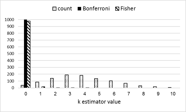
For the examples of this section we synthesize values to emulate a test with hypotheses (domains), and set to 0.05. We start with a simulation of a scenario where algorithm is equivalent to for each domain, and the datasets representing these domains are independent. We sample the 100 values from a standard uniform distribution, which is the value distribution under the null hypothesis, repeating the simulation 1000 times.
Since all the null hypotheses are true then , the number of false null hypotheses, is . Figure 1 presents the histogram of values from all 1000 iterations according to , and .
The figure clearly demonstrates that provides an overestimation of while and do much better. Indeed, the histogram yields the following probability estimates: , and (only the latter two are lower than 0.05). This simulation strongly supports the theoretical results of Section 4.2.
To consider a scenario where a dependency between the participating datasets does exist, we consider a second toy example. In this example we generate values corresponding to 34 independent normal test statistics, and two other groups of 33 positively correlated normal test statistics with and , respectively. We again assume that all null hypotheses are true and thus all the values are distributed uniformly, repeating the simulation 1000 times. To generate positively dependent values we followed the process described in Section 6.1 of ?).
We estimate the probability that for the three estimators based on the 1000 repetitions and get the values of: , and . This simulation demonstrates the importance of using Bonferroni’s method rather than Fisher’s method when the datasets are dependent, even if some of the datasets are independent.
6 NLP Applications
In this section we demonstrate the potential impact of replicability analysis on the way experimental results are analyzed in NLP setups. We explore four NLP applications: (a) two where the datasets are independent: multi-domain dependency parsing and multilingual POS tagging; and (b) two where dependency between the datasets does exist: cross-domain sentiment classification and word similarity prediction with word embedding models.
6.1 Data
Dependency Parsing
We consider a multi-domain setup, analyzing the results reported in ?). The authors compared ten state-of-the-art parsers from which we pick three: (a) Mate [Bohnet (2010]888code.google.com/p/mate-tools. that performed best on the majority of datasets; (b) Redshift [Honnibal et al. (2013]999github.com/syllog1sm/Redshift. which demonstrated comparable, still somewhat lower, performance compared to Mate; and (c) SpaCy [Honnibal and Johnson (2015]101010honnibal.github.io/spaCy. that was substantially outperformed by Mate.
All parsers were trained and tested on the English portion of the OntoNotes 5 corpus [Weischedel et al. (2011, Pradhan et al. (2013], a large multi-genre corpus consisting of the following 7 genres: broadcasting conversations (BC), broadcasting news (BN), news magazine (MZ), newswire (NW), pivot text (PT), telephone conversations (TC) and web text (WB). Train and test set size (in sentences) range from 6672 to 34492 and from 280 to 2327, respectively (see Table 1 of [Choi et al. (2015]). We copy the test set UAS results of ?) and compute values using the data downloaded from http://amandastent.com/dependable/.
POS Tagging
We consider a multilingual setup, analyzing the results reported in [Pinter et al. (2017]. The authors compare their Mimick model with the model of ?), denoted with chartag. Evaluation is performed on 23 of the 44 languages shared by the Polyglot word embedding dataset [Al-Rfou et al. (2013] and the universal dependencies (UD) dataset [De Marneffe et al. (2014]. ?) choose their languages so that they reflect a variety of typological, and particularly morphological, properties. The training/test split is the standard UD split. We copy the word level accuracy figures of [Pinter et al. (2017] for the low resource training set setup, the focus setup of that paper. The authors kindly sent us their -values.
Sentiment Classification
In this task, an algorithm is trained on reviews from one domain and should classify the sentiment of reviews from another domain to the positive and negative classes. For replicability analysis we explore the results of ?) for the cross-domain sentiment classification task of ?). The data in this task consists of Amazon product reviews from 4 domains: books (B), DVDs (D), electronic items (E), and kitchen appliances (K), for the total of 12 domain pairs, each domain having a 2000 review test set.111111http://www.cs.jhu.edu/~mdredze/datasets/sentiment/index2.htm ?) compared the accuracy of their AE-SCL-SR model to MSDA [Chen et al. (2011], a well known domain adaptation method, and kindly sent us the required -values.
Word Similarity
We compare two state-of-the-art word embedding collections: (a) word2vec CBOW [Mikolov et al. (2013] vectors, generated by the model titled the best ”predict” model in ?);121212http://clic.cimec.unitn.it/composes/semantic-vectors.html. Parameters: 5-word context window, 10 negative samples, subsampling, 400 dimensions. and (b) Glove [Pennington et al. (2014] vectors generated by a model trained on a 42B token common web crawl.131313http://nlp.stanford.edu/projects/glove/. 300 dimensions. We employed the demo of ?) to perform Spearman correlation evaluation of these vector collections on 12 English word pair datasets: WS-353 [Finkelstein et al. (2001b], WS-353-SIM [Agirre et al. (2009], WS-353-REL [Agirre et al. (2009], MC-30 [Miller and Charles (1991], RG-65 [Rubenstein and Goodenough (1965], Rare-Word [Luong et al. (2013], MEN [Bruni et al. (2012], MTurk-287 [Radinsky et al. (2011], MTurk-771 [Halawi et al. (2012], YP-130 [Yang and Powers (], SimLex-999 [Hill et al. (2016], and Verb-143 [Baker et al. (2014].
6.2 Statistical Significance Tests
We first calculate the values for each task and dataset according to the principals of values computation for NLP discussed in ?), ?) and ?).
For dependency parsing, we employ the a-parametric paired bootstrap test [Efron and Tibshirani (1994] that does not assume any distribution on the test statistics. We choose this test because the distribution of the values for the measures commonly applied in this task is unknown. We implemented the test as in [Berg-Kirkpatrick et al. (2012] with a bootstrap size of 500 and with repetitions.
For multilingual POS tagging we employ the Wilcoxon signed-rank test [Wilcoxon (1945]. The test is employed for the sentence level accuracy scores of the two compared models. This test is a non-parametric test for difference in measures, which tests the null hyphotesis that the difference has a symmetric distribution around zero. It is appropriate for tasks with paired continuous measures for each observation, which is the case when comparing sentence level accuracies.
For sentiment classification we employ the McNemar test for paired nominal data [McNemar (1947]. This test is appropriate for binary classification tasks and since we compare the results of the algorithms when applied on the same datasets, we employ its paired version. Finally, for word similarity with its Spearman correlation evaluation, we choose the Steiger test [Steiger (1980] for comparing elements in a correlation matrix.
We consider the case of for all four applications. For the dependent datasets experiments (sentiment classification and word similarity prediction) with their generally lower values (see below), we also consider the case where .
6.3 Results
| Independent Datasets | |||
| Dependency Parsing (7 datasets) | |||
| Mate-SpaCy | 7 | 7 | 7 |
| Mate-Redshift | 2 | 1 | 5 |
| Multilingual POS Tagging (23 datasets) | |||
| Mimick-CharTag | 11 | 6 | 16 |
| Dependent Datasets | |||
| Sentiment Classification (12 setups) | |||
| AE-SCL-SR-MSDA | 10 | 6 | 10 |
| () | |||
| AE-SCL-SR-MSDA | 6 | 2 | 8 |
| () | |||
| Word Similarity (12 datasets) | |||
| W2V-Glove | 8 | 6 | 7 |
| () | |||
| W2V-Glove | 6 | 4 | 6 |
| () | |||
| Model Data | BC | BN | MZ | NW | PT | TC | WB |
| Mate | 90.73 | 90.82 | 91.92 | 91.68 | 96.64 | 89.87 | 89.89 |
| SpaCy | 89.05 | 89.31 | 89.29 | 89.52 | 95.27 | 87.65 | 87.40 |
| val (Mate,SpaCy) | () | () | (0.0) | (0.0) | () | () | (0.0) |
| Redshift | 90.19 | 90.46 | 90.90 | 90.99 | 96.22 | 88.99 | 89.31 |
| val (Mate,Redshift) | (0.0979) | (0.1662) | (0.0046) | (0.0376) | (0.0969) | (0.0912) | (0.0823) |
| Language | Mimick | CharTag | value |
| Kazakh | 83.95 | 83.64 | 0.0944 |
| Tamil∗ | 81.55 | 84.97 | 0.0001 |
| Latvian | 84.32 | 84.49 | 0.0623 |
| Vietnamese | 84.22 | 84.85 | 0.0359 |
| Hungarian∗ | 88.93 | 85.83 | 1.12e-08 |
| Turkish | 85.60 | 84.23 | 0.1461 |
| Greek | 93.63 | 94.05 | 0.0104 |
| Bulgarian | 93.16 | 93.03 | 0.1957 |
| Swedish | 92.30 | 92.27 | 0.0939 |
| Basque∗ | 84.44 | 86.01 | 3.87e-10 |
| Russian | 89.72 | 88.65 | 0.0081 |
| Danish | 90.13 | 89.96 | 0.1016 |
| Indonesian∗ | 89.34 | 89.81 | 0.0008 |
| Chinese∗ | 85.69 | 81.84 | 0 |
| Persian | 93.58 | 93.53 | 0.4450 |
| Hebrew | 91.69 | 91.93 | 0.1025 |
| Romanian | 89.18 | 88.96 | 0.2198 |
| English | 88.45 | 88.89 | 0.0208 |
| Arabic | 90.58 | 90.49 | 0.0731 |
| Hindi | 87.77 | 87.92 | 0.0288 |
| Italian | 92.50 | 92.45 | 0.4812 |
| Spanish | 91.41 | 91.71 | 0.1176 |
| Czech∗ | 90.81 | 90.17 | 2.91e-05 |
| Dataset | AE-SCL-SR | MSDA | value |
|---|---|---|---|
| 0.8005 | 0.788 | 0.0268 | |
| 0.8105 | 0.783 | 0.0011 | |
| 0.7675 | 0.7455 | 0.0119 | |
| 0.7295 | 0.7 | 0.0038 | |
| 0.763 | 0.714 | 1.9e-06 | |
| 0.84 | 0.824 | 0.018 | |
| 0.773 | 0.7605 | 0.0186 | |
| 0.8025 | 0.774 | 0.0014 | |
| 0.781 | 0.75 | 0.0011 | |
| 0.7115 | 0.7185 | 0.4823 | |
| 0.8455 | 0.845 | 0.9507 | |
| 0.745 | 0.71 | 0.0003 |
| Dataset | W2V | GLOVE | val. |
|---|---|---|---|
| WS353∗,+ | 0.7362 | 0.629 | |
| WS353-SIM∗,+ | 0.7805 | 0.6979 | 0.0 |
| WS353-REL | 0.6814 | 0.5706 | 0.2123 |
| MC-30∗,+ | 0.8221 | 0.7773 | 0.0001 |
| RG-65 | 0.8348 | 0.8117 | 0.3053 |
| RW | 0.4819 | 0.4144 | 0.2426 |
| MEN∗ | 0.796 | 0.7362 | 0.0021 |
| MTurk-287 | 0.671 | 0.6475 | 0.2076 |
| MTurk-771 | 0.7116 | 0.6842 | 0.0425 |
| YP-130∗,+ | 0.504 | 0.5315 | 0.0 |
| SimLex999∗ | 0.4621 | 0.3725 | 0.0015 |
| 0.4479 | 0.3275 | 0.0431 |
Table 1 summarizes the replicability analysis results while Table 2 – 5 present task specific performance measures and values.
Independent Datasets
Dependency parsing (Tab. 2) and multilingual POS tagging (Tab. 3) are our example tasks for this setup, where is our recommended valid estimator for the number of cases where one algorithm outperforms another.
For dependency parsing, we compare two scenarios: (a) where in most domains the differences between the compared algorithms are quite large and the values are small (Mate vs. SpaCy); and (b) where in most domains the differences between the compared algorithms are smaller and the values are higher (Mate vs. Redshift). Our multilingual POS tagging scenario (Mimick vs. CharTag) is more similar to scenario (b) in terms of the differences between the participating algorithms.
Table 1 demonstrates the estimators for the various tasks and scenarios. For dependency parsing, as expected, in scenario (a) where all the values are small, all estimators, even the error-prone , provide the same information. In case (b) of dependency parsing, however, estimates the number of domains where Mate outperforms Redshift to be 5, while estimates this number to be only 2. This is a substantial difference given that the total number of domains is 7. The estimator, that is valid under arbitrary dependencies and does not exploit the independence assumption as does, is even more conservative than and its estimation is only 1.
Perhaps not surprisingly, the multilingual POS tagging results are similar to case (b) of dependency parsing. Here, again, is too conservative, estimating the number of languages with effect to be 11 (out of 23) while estimates this number to be 16 (an increase of 5/23 in the estimated number of languages with effect). is again more conservative, estimating the number of languages with effect to be only 6, which is not very surprising given that it does not exploit the independence between the datasets. These two examples of case (b) demonstrate that when the differences between the algorithms are quite small, may be more sensitive than the current practice in NLP for discovering the number of datasets with effect.
To complete the analysis, we would like to name the datasets with effect. As discussed in Section 4.2, while this can be straightforwardly done by naming the datasets with the smallest values, in general, this approach does not control the probability of identifying at least one dataset erroneously. We thus employ the Holm procedure for the identification task, noticing that the number of datasets it identifies should be equal to the value of the estimator (Section 4.3).
Indeed, for dependency parsing in case (a), the Holm procedure identifies all seven domains as cases where Mate outperforms SpaCy, while in case (b) it identifies only the MZ domain as a case where Mate outperforms Redshift. For multilingual POS tagging the Holm procedure identifies Tamil, Hungarian, Basque, Indonesian, Chinese and Czech as languages where Mimick outperforms CharTag. Expectedly, this analysis demonstrates that when the performance gap between two algorithms becomes narrower, inquiring for more information (i.e. identifying the domains with effect rather than just estimating their number), may come at the cost of weaker results.141414For completeness, we also performed the analysis for the independent dataset setups with . The results are (, , ): Mate vs. Spacy: (7,7,7); Mate vs. Redshift (1,0,2); Mimick vs. CharTag: (7,5,13). The patterns are very similar to those discussed in the text.
Dependent Datasets
In cross-domain sentiment classification (Table 4) and word similarity prediction (Table 5), the involved datasets manifest mutual dependence. Particularly, each sentiment setup shares its test dataset with 2 other setups, while in word similarity WS-353 is the union of WS-353-REL and WS-353-SIM. As discussed in Section 4, is the appropriate estimator of the number of cases one algorithm outperforms another.
The results in Table 1 manifest the phenomenon demonstrated by the second toy example in Section 5, which shows that when the datasets are dependent, as well as the error-prone may be too optimistic regarding the number of datasets with effect. This stands in contrast to that controls the probability to overestimate the number of such datasets.
Indeed, is much more conservative, yielding values of 6 ( = 0.05) and 2 ( = 0.01) for sentiment, and of 6 ( = 0.05) and 4 ( = 0.01) for word similarity. The differences from the conclusions that might have been drawn by are again quite substantial. The difference between and in sentiment classification is 4, which accounts to 1/3 of the 12 test setups. Even for word similarity, the difference between the two methods, which account to 2 for both values, represents 1/6 of the 12 test setups. The domains identified by the Holm procedure are marked in the tables.
Results Overview
Our goal in this section is to demonstrate that the approach of simply looking at the number of datasets for which the difference between the performance of the algorithms reaches a predefined significance level, gives different results from our suggested statistically sound analysis. This approach is denoted here with and shown to be statistically not valid in Sections 3.2 and 5. We observe that this happens especially in evaluation setups where the differences between the algorithms are small for most datasets. In some cases, when the datasets are independent, our analysis has the power to declare a larger number of datasets with effect than the number of individual significant test values (). In other cases, when the datasets are interdependent, is much too optimistic.
Our proposed analysis changes the observations that might have been made based on the papers where the results analysed here were originally reported. For example, for the Mate-Redshift comparison (independent evaluation sets), we show that there is evidence that the number of datasets with effect is much higher than one would assume based on counting the significant sets (5 vs. 2 out of 7 evaluation sets), giving a stronger claim regarding the superiority of Mate. In multingual POS tagging (again, an independent evaluation sets setup) our analysis shows evidence for 16 sets with effect compared to only 11 of the erroneous count method - a difference in 5 out of 23 evaluation sets (21.7%). Finally, in the cross-domain sentiment classification and the word similarity judgment tasks (dependent evaluation sets), the unjustified counting method may be too optimistic (e.g. 10 vs. 6 out of 12 evaluation sets, for in the sentiment task), in favor of the new algorithms.
7 Discussion and Future Directions
We proposed a statistically sound replicability analysis framework for cases where algorithms are compared across multiple datasets. Our main contributions are: (a) analyzing the limitations of the current practice in NLP work: counting the datasets for which the difference between the algorithms reaches a predefined significance level; and (b) proposing a new framework that addresses both the estimation of the number of datasets with effect and the identification of such datasets.
The framework we propose addresses two different situations encountered in NLP: independent and dependent datasets. For dependent datasets, we assumed that the type of dependency cannot be determined. One could use more powerful methods if certain assumptions on the dependency between the test statistics could be made. For example, one could use the partial conjunction p-value based on Simes test for the global null hypothesis [Simes (1986], which was proposed by [Benjamini and Heller (2008] for the case where the test statistics satisfy certain positive dependency properties (see Theorem 1 in [Benjamini and Heller (2008]). Using this partial conjunction p-value rather than the one based on Bonferroni, one may obtain higher values of with the same statistical guarantee. Similarly, for the identification question, if certain positive dependency properties hold, Holm’s procedure could be replaced by Hochberg’s or Hommel’s procedures [Hochberg (1988, Hommel (1988] which are more powerful.
An alternative, more powerful multiple testing procedure for identification of datasets with effect, is the method in ?), that controls the false discovery rate (FDR), a less strict error criterion than the one considered here. This method is more appropriate in cases where one may tolerate some errors as long as the proportion of errors among all the claims made is small, as expected to happen when the number of datasets grows.
We note that the increase in the number of evaluation datasets may have positive and negative aspects. As noted in Section 2, we believe that multiple comparisons are integral to NLP research when aiming to develop algorithms that perform well across languages and domains. On the other hand, experimenting with multiple evaluation sets that reflect very similar linguistic phenomena may only complicate the comparison between alternative algorithms.
In fact, our analysis is useful mostly where the datasets are heterogeneous, coming from different languages or domains. When they are just technically different but could potentially be just combined into a one big dataset, then we believe the question of ?), whether at least one dataset shows evidence for effect, is more appropriate.
Acknowledgement
The research of M. Bogomolov was supported by the Israel Science Foundation grant No. 1112/14. We thank Yuval Pinter for his great help with the multilingual experiments and for his useful feedback. We also thank Ruth Heller, Marten van Schijndel, Oren Tsur, Or Zuk and the ie@technion NLP group members for their useful comments.
References
- [Agirre et al. (2009] Eneko Agirre, Enrique Alfonseca, Keith Hall, Jana Kravalova, Marius Paşca, and Aitor Soroa. 2009. A study on similarity and relatedness using distributional and wordnet-based approaches. In Proceedings of HLT-NAACL.
- [Al-Rfou et al. (2013] Rami Al-Rfou, Bryan Perozzi, and Steven Skiena. 2013. Polyglot: Distributed word representations for multilingual nlp. In Proceedings of CoNLL.
- [Baker et al. (2014] Simon Baker, Roi Reichart, and Anna Korhonen. 2014. An unsupervised model for instance level subcategorization acquisition. In Proceedings of EMNLP.
- [Baroni et al. (2014] Marco Baroni, Georgiana Dinu, and Germán Kruszewski. 2014. Don’t count, predict! a systematic comparison of context-counting vs. context-predicting semantic vectors. In Proceedings of ACL.
- [Begley and Ellis (2012] C. Glenn Begley and Lee M. Ellis. 2012. Drug development: Raise standards for preclinical cancer research. Nature, 483(7391):531–533.
- [Benjamini and Heller (2008] Yoav Benjamini and Ruth Heller. 2008. Screening for partial conjunction hypotheses. Biometrics, 64(4):1215–1222.
- [Benjamini and Hochberg (1995] Yoav Benjamini and Yosef Hochberg. 1995. Controlling the false discovery rate: A practical and powerful approach to multiple testing. Journal of the royal statistical society. Series B (Methodological), pages 289–300.
- [Benjamini et al. (2006] Yoav Benjamini, Abba M. Krieger, and Daniel Yekutieli. 2006. Adaptive linear step-up procedures that control the false discovery rate. Biometrika, pages 491–507.
- [Benjamini et al. (2009] Yoav Benjamini, Ruth Heller, and Daniel Yekutieli. 2009. Selective inference in complex research. Philosophical Transactions of the Royal Society of London A: Mathematical, Physical and Engineering Sciences, 367(1906):4255–4271.
- [Berg-Kirkpatrick et al. (2012] Taylor Berg-Kirkpatrick, David Burkett, and Dan Klein. 2012. An empirical investigation of statistical significance in nlp. In Proceedings of EMNLP-CoNLL.
- [Blitzer et al. (2006] John Blitzer, Ryan McDonald, and Fernando Pereira. 2006. Domain adaptation with structural correspondence learning. In Proceedings of EMNLP.
- [Blitzer et al. (2007] John Blitzer, Mark Dredze, and Fernando Pereira. 2007. Biographies, bollywood, boom-boxes and blenders: Domain adaptation for sentiment classification. In Proceedings of ACL.
- [Bohnet (2010] Bernd Bohnet. 2010. Very high accuracy and fast dependency parsing is not a contradiction. In Proceedings of COLING.
- [Bruni et al. (2012] Elia Bruni, Gemma Boleda, Marco Baroni, and Nam-Khanh Tran. 2012. Distributional semantics in technicolor. In Proceedings of ACL.
- [Bruni et al. (2014] Elia Bruni, Nam-Khanh Tran, and Marco Baroni. 2014. Multimodal distributional semantics. Journal of Artificial Intelligence Research (JAIR), 49:1–47.
- [Buchholz and Marsi (2006] Sabine Buchholz and Erwin Marsi. 2006. Conll-x shared task on multilingual dependency parsing. In Proceedings of CoNLL.
- [Chan and Ng (2007] Yee Seng Chan and Hwee Tou Ng. 2007. Domain adaptation with active learning for word sense disambiguation. In Proceedings of ACL.
- [Charniak (2000] Eugene Charniak. 2000. A maximum-entropy-inspired parser. In Proceedings of HLT-NAACL.
- [Chen et al. (2011] Minmin Chen, Yixin Chen, and Kilian Q. Weinberger. 2011. Automatic feature decomposition for single view co-training. In Proceedings of ICML.
- [Choi et al. (2015] Jinho D Choi, Joel Tetreault, and Amanda Stent. 2015. It depends: Dependency parser comparison using a web-based evaluation tool. In Proceedings of ACL.
- [Collaboration (2012] Open Science Collaboration. 2012. An open, large-scale, collaborative effort to estimate the reproducibility of psychological science. Perspectives on Psychological Science, 7(6):657–660.
- [Collins (2003] Michael Collins. 2003. Head-driven statistical models for natural language parsing. Computational linguistics, 29(4):589–637.
- [Daumé III (2007] Hal Daumé III. 2007. Frustratingly easy domain adaptation. In Proceedings of ACL.
- [De Marneffe et al. (2014] Marie-Catherine De Marneffe, Timothy Dozat, Natalia Silveira, Katri Haverinen, Filip Ginter, Joakim Nivre, and Christopher D. Manning. 2014. Stanford dependencies: A cross-linguistic typology. In Proceedings of LREC.
- [Demšar (2006] Janez Demšar. 2006. Statistical comparisons of classifiers over multiple data sets. Journal of Machine learning research, 7(Jan):1–30.
- [Dietterich (1998] Thomas G. Dietterich. 1998. Approximate statistical tests for comparing supervised classification learning algorithms. Neural computation, 10(7):1895–1923.
- [Efron and Tibshirani (1994] Bradley Efron and Robert J. Tibshirani. 1994. An introduction to the bootstrap. CRC press.
- [Farcomeni (2007] Alessio Farcomeni. 2007. A review of modern multiple hypothesis testing, with particular attention to the false discovery proportion. Statistical Methods in Medical Research.
- [Faruqui and Dyer (2014] Manaal Faruqui and Chris Dyer. 2014. Community evaluation and exchange of word vectors at wordvectors.org. In Proceedings of the ACL: System Demonstrations.
- [Finkelstein et al. (2001a] Lev Finkelstein, Evgeniy Gabrilovich, Yossi Matias, Ehud Rivlin, Zach Solan, Gadi Wolfman, and Eytan Ruppin. 2001a. Placing search in context: The concept revisited. In Proc. of WWW.
- [Finkelstein et al. (2001b] Lev Finkelstein, Evgeniy Gabrilovich, Yossi Matias, Ehud Rivlin, Zach Solan, Gadi Wolfman, and Eytan Ruppin. 2001b. Placing search in context: The concept revisited. In Proceedings of WWW.
- [Guo et al. (2009] Honglei Guo, Huijia Zhu, Zhili Guo, Xiaoxun Zhang, Xian Wu, and Zhong Su. 2009. Domain adaptation with latent semantic association for named entity recognition. In Proceedings of HLT-NAACL.
- [Halawi et al. (2012] Guy Halawi, Gideon Dror, Evgeniy Gabrilovich, and Yehuda Koren. 2012. Large-scale learning of word relatedness with constraints. In Proceedings of ACM SIGKDD.
- [Heller et al. (2014] Ruth Heller, Marina Bogomolov, and Yoav Benjamini. 2014. Deciding whether follow-up studies have replicated findings in a preliminary large-scale omics study. Proceedings of the National Academy of Sciences, 111(46):16262–16267.
- [Herndon et al. (2014] Thomas Herndon, Michael Ash, and Robert Pollin. 2014. Does high public debt consistently stifle economic growth? a critique of reinhart and rogoff. Cambridge journal of economics, 38(2):257–279.
- [Hill et al. (2015] Felix Hill, Roi Reichart, and Anna Korhonen. 2015. Simlex-999: Evaluating semantic models with (genuine) similarity estimation. Computational Linguistics, 41(4):665–695.
- [Hill et al. (2016] Felix Hill, Roi Reichart, and Anna Korhonen. 2016. Simlex-999: Evaluating semantic models with (genuine) similarity estimation. Computational Linguistics.
- [Hochberg (1988] Yosef Hochberg. 1988. A sharper bonferroni procedure for multiple tests of significance. Biometrika, 75(4):800–802.
- [Holm (1979] Sture Holm. 1979. A simple sequentially rejective multiple test procedure. Scandinavian Journal of Statistics, 6(2):65–70.
- [Hommel (1988] Gerhard Hommel. 1988. A stagewise rejective multiple test procedure based on a modified bonferroni test. Biometrika, 75(2):383–386.
- [Honnibal and Johnson (2015] Matthew Honnibal and Mark Johnson. 2015. An improved non-monotonic transition system for dependency parsing. In Proceedings of EMNLP.
- [Honnibal et al. (2013] Matthew Honnibal, Yoav Goldberg, and Mark Johnson. 2013. A non-monotonic arc-eager transition system for dependency parsing. In Proceedings of CoNLL.
- [Koehn and Schroeder (2007] Philipp Koehn and Josh Schroeder. 2007. Experiments in domain adaptation for statistical machine translation. In Proceedings of the second workshop on statistical machine translation.
- [Koehn (2005] Philipp Koehn. 2005. Europarl: A parallel corpus for statistical machine translation. In Proceedings of the tenth Machine Translation Summit.
- [Leek and Peng (2015] Jeffrey T. Leek and Roger D Peng. 2015. Opinion: Reproducible research can still be wrong: Adopting a prevention approach. Proceedings of the National Academy of Sciences, 112(6):1645–1646.
- [Levy and Goldberg (2014] Omer Levy and Yoav Goldberg. 2014. Dependency-based word embeddings. In Proceedings of ACL.
- [Ling et al. (2015] Wang Ling, Chris Dyer, Alan W. Black, Isabel Trancoso, Ramon Fermandez, Silvio Amir, Luis Marujo, and Tiago Luis. 2015. Finding function in form: Compositional character models for open vocabulary word representation. In Proceedings of EMNLP.
- [Loughin (2004] Thomas M. Loughin. 2004. A systematic comparison of methods for combining p-values from independent tests. Computational statistics & data analysis, 47(3):467–485.
- [Luong et al. (2013] Minh-Thang Luong, Richard Socher, and Christopher D. Manning. 2013. Better word representations with recursive neural networks for morphology. In Proceedings of CoNLL.
- [Marcus et al. (1993] Mitchell P. Marcus, Mary Ann Marcinkiewicz, and Beatrice Santorini. 1993. Building a large annotated corpus of english: The penn treebank. Computational linguistics, 19(2):313–330.
- [Marrese-Taylor and Matsuo (2017] Edison Marrese-Taylor and Yutaka Matsuo. 2017. Replication issues in syntax-based aspect extraction for opinion mining. In Proceedings of the Student Research Workshop at EACL.
- [McNemar (1947] Quinn McNemar. 1947. Note on the sampling error of the difference between correlated proportions or percentages. Psychometrika, 12(2):153–157.
- [Mikolov et al. (2013] Tomas Mikolov, Ilya Sutskever, Kai Chen, Gregory S. Corrado, and Jeffrey Dean. 2013. Distributed representations of words and phrases and their compositionality. In Proceedings of NIPS.
- [Miller and Charles (1991] George A. Miller and Walter G. Charles. 1991. Contextual correlates of semantic similarity. Language and cognitive processes, 6(1):1–28.
- [Moonesinghe et al. (2007] Ramal Moonesinghe, Muin J. Khoury, and A. Cecile J. W. Janssens. 2007. Most published research findings are false—but a little replication goes a long way. PLoS Med, 4(2):e28.
- [Névéol et al. (2016] Aurélie Névéol, Cyril Grouin, Kevin Bretonnel Cohen, and Aude Robert. 2016. Replicability of research in biomedical natural language processing: a pilot evaluation for a coding task. Proceedings of EMNLP.
- [Nilsson et al. (2007] Jens Nilsson, Sebastian Riedel, and Deniz Yuret. 2007. The conll 2007 shared task on dependency parsing. In Proceedings of CoNLL.
- [Ó Séaghdha and Korhonen (2014] Diarmuid Ó Séaghdha and Anna Korhonen. 2014. Probabilistic distributional semantics. Computational Linguistics, 40(3):587–631.
- [Patil et al. (2016] Prasad Patil, Roger D. Peng, and Jeffrey Leek. 2016. A statistical definition for reproducibility and replicability. bioRxiv.
- [Peng (2011] Roger D. Peng. 2011. Reproducible research in computational science. Science, 334(6060):1226–1227.
- [Pennington et al. (2014] Jeffrey Pennington, Richard Socher, and Christopher Manning. 2014. GloVe: Global vectors for word representation. In Proceedings of EMNLP.
- [Petrov and McDonald (2012] Slav Petrov and Ryan McDonald. 2012. Overview of the 2012 shared task on parsing the web. In Notes of the First Workshop on Syntactic Analysis of Non-Canonical Language (SANCL).
- [Pinter et al. (2017] Yuval Pinter, Robert Guthrie, and Jacob Eisenstein. 2017. Mimicking word embeddings using subword rnns. In Proceedings of EMNLP.
- [Pradhan et al. (2013] Sameer Pradhan, Alessandro Moschitti, Nianwen Xue, Hwee Tou Ng, Anders Björkelund, Olga Uryupina, Yuchen Zhang, and Zhi Zhong. 2013. Towards robust linguistic analysis using ontonotes. In Proceedings of CoNLL.
- [Radinsky et al. (2011] Kira Radinsky, Eugene Agichtein, Evgeniy Gabrilovich, and Shaul Markovitch. 2011. A word at a time: Computing word relatedness using temporal semantic analysis. In Proceedings of WWW.
- [Rubenstein and Goodenough (1965] Herbert Rubenstein and John B. Goodenough. 1965. Contextual correlates of synonymy. Communications of the ACM, 8(10):627–633.
- [Schwartz et al. (2015] Roy Schwartz, Roi Reichart, and Ari Rappoport. 2015. Symmetric pattern based word embeddings for improved word similarity prediction. In Proceedings of CoNLL.
- [Silberer and Lapata (2014] Carina Silberer and Mirella Lapata. 2014. Learning grounded meaning representations with autoencoders. In Proceedings of ACL.
- [Simes (1986] R John Simes. 1986. An improved bonferroni procedure for multiple tests of significance. Biometrika, pages 751–754.
- [Snow et al. (2008] Rion Snow, Brendan O’Connor, Daniel Jurafsky, and Andrew Y. Ng. 2008. Cheap and fast—but is it good?: Evaluating non-expert annotations for natural language tasks. In Proceedings of EMNLP.
- [Søgaard et al. (2014] Anders Søgaard, Anders Johannsen, Barbara Plank, Dirk Hovy, and Héctor Martínez Alonso. 2014. What’s in a p-value in nlp? In Proceedings of CoNLL.
- [Søgaard (2013] Anders Søgaard. 2013. Estimating effect size across datasets. In Proceedings of HLT-NAACL.
- [Steiger (1980] James H. Steiger. 1980. Tests for comparing elements of a correlation matrix. Psychological bulletin, 87(2):245–251.
- [Weischedel et al. (2011] Ralph Weischedel, Eduard Hovy, Mitchell Marcus, Martha Palmer, Robert Belvin, Sameer Pradhan, Lance Ramshaw, and Nianwen Xue. 2011. Ontonotes: A large training corpus for enhanced processing. Handbook of Natural Language Processing and Machine Translation. Springer.
- [Wilcoxon (1945] Frank Wilcoxon. 1945. Individual comparisons by ranking methods. Biometrics bulletin, 1(6):80–83.
- [Yang and Powers (] Dongqiang Yang and David MW. Powers. Verb similarity on the taxonomy of wordnet. In Proceedings of the 3rd International WordNet Conference.
- [Yeh (2000] Alexander Yeh. 2000. More accurate tests for the statistical significance of result differences. In Proceedings of CoNLL.
- [Ziser and Reichart (2017] Yftah Ziser and Roi Reichart. 2017. Neural structural correspondence learning for domain adaptation. In Proceedings of CoNLL.