11email: lama.affara@kaust.edu.sa, bernard.ghanem@kaust.edu.sa, pwonka@gmail.com
Fast Convolutional Sparse Coding in the Dual Domain
Abstract
Convolutional sparse coding (CSC) is an important building block of many computer vision applications ranging from image and video compression to deep learning. We present two contributions to the state of the art in CSC. First, we significantly speed up the computation by proposing a new optimization framework that tackles the problem in the dual domain. Second, we extend the original formulation to higher dimensions in order to process a wider range of inputs, such as RGB images and videos. Our results show up to 20 times speedup compared to current state-of-the-art CSC solvers.
1 Introduction
Human vision is characterized by the response of neurons to stimuli within their receptive fields, which is usually modeled mathematically by the convolution operator. Correspondingly for computer vision, coding the image based on a convolutional model has shown its benefits through the development and application of deep Convolutional Neural Networks. Such a model constitutes a strategy for unsupervised feature learning, and more specifically to patch-based feature learning also known as dictionary learning.
Convolutional Sparse Coding (CSC) is a special type of sparse dictionary learning algorithms. It uses the convolution operator in its image representation model rather than generic linear combinations. This results in diverse translation-invariant patches and maintains the latent structures of the underlying signal. CSC has recently been applied in a wide range of computer vision problems such as image and video processing [1, 2, 3, 4, 5], structure from motion [6], computational imaging [7], tracking [8], as well as the design of deep learning architectures [9].
Finding an efficient solution to the CSC problem however is a challenging task due to its high computational complexity and the non-convexity of its objective function. Seminal advances [10, 11, 12] in CSC have shown computational speed-up by solving the problem efficiently in the Fourier domain where the convolution operator is transformed to element-wise multiplication. As such, the optimization is modeled as a biconvex problem formed by two convex subproblems, the coding subproblem and the learning subproblem, that are iteratively solved in a fixed point manner.
Despite the performance boost attained by solving the CSC optimization problem in the Fourier domain, the problem is still computationally expensive due to the dominating cost of solving large linear systems. More recent work [12, 11] makes use of the block-diagonal structure of the matrices involved and solves the linear systems in a parallel fashion, thus leveraging hardware acceleration.
Inspired by recent work on circulant sparse trackers [8], we model the CSC problem in the dual domain. The dual formulation casts the coding subproblem into an Alternating Direction Method of Multipliers (ADMM) framework that involves solving a linear system with a lower number of parameters than previous work. This allows our algorithm to achieve not only faster convergence towards a feasible solution, but also a lower computational cost. The solution for the learning subproblem in the dual domain is achieved by applying coordinate ascent over the Lagrange multipliers and the dual parameters. Our extensive experiments show that the dual framework achieves significant speedup over the state of the art while converging to comparable objective values.
Moreover, recent work on higher order tensor formulations for CSC (TCSC) handles the problem with an arbitrary order tensor of data which allows learning more elaborate dictionaries such as colored dictionaries. This allows a richer image representation and greatly benefits the applicability of CSC in other application domains such as color video reconstruction. Our dual formulation provides faster performance compared to TCSC by eliminating the need for solving a large number of linear systems involved in the coding subproblem which dominates the cost for solving the problem.
Contributions. We present two main contributions. (1) We formulate the CSC problem in the dual domain and show that this formulation leads to faster convergence and thus lower computation time. (2) We extend our dual formulation to higher dimensions and gain up to 20 times speedup compared to TCSC.
2 Related Work
As mentioned earlier, CSC has many applications and quite a few methods have been proposed to solve the non-convex CSC optimization. In the following, we mainly review the works that focus on the computational complexity and efficiency aspects of the problem.
The seminal work of [13] proposes Deconvolutional Networks, a learning framework based on convolutional decomposition of images under a sparsity constraint. Unlike previous work in sparse image decomposition [14, 15, 16, 17] that builds hierarchical representations of an image on a patch level, Deconvolutional Networks perform a sparse decomposition over entire images. This strategy significantly reduces the redundancy among filters compared with those obtained by the patch-based approaches. Kavukcuoglu et al. [18] propose a convolutional extension to the coordinate descent sparse coding algorithm [19] to represent images using convolutional dictionaries for object recognition tasks. Following this path, Yang et al. [20] propose a supervised dictionary learning approach to improve the efficiency of sparse coding.
To efficiently solve the complex optimization problems in CSC, most existing solvers attempt to transform the problem into the frequency domain. Šorel and Šroubek [21] propose a non-iterative method for computing the inversion of the convolutional operator in the Fourier domain using the matrix inversion lemma. Bristow et al. [10] propose a quad-decomposition of the original objective into convex subproblems and exploit the ADMM approach to solve the convolution subproblems in the Fourier domain. In their follow-up work [22], a number of optimization methods for solving convolution problems and their applications are discussed. In the work of [11], the authors further exploit the separability of convolution across bands in the frequency domain. Their gain in efficiency arises from computing a partial vector (instead of a full vector). To further improve efficiency, Heide et al. [12] transform the original constrained problem into an unconstrained problem by encoding the constraints in the objective using some indicator functions. The new objective function is then further split into a set of convex functions that are easier to optimize separately. They also devise a more flexible solution by adding a diagonal matrix to the objective function to handle the boundary artifacts resulting from transforming the problem into the Fourier domain.
Various CSC methods have also been proposed for different applications. Zhang et al. [8] propose an efficient sparse coding method for sparse tracking. They also solve the problem in the Fourier domain, in which the optimization is obtained by solving its dual problem and thus achieving more efficient computation. Unlike traditional sparse coding based image super resolution methods that divide the input image into overlapping patches, Gu et al. [5] propose to decompose the image by filtering. Their method is capable of reconstructing local image structures. Similar to [10], the authors also solve the subproblems in the Fourier domain. The stochastic average and ADMM algorithms [23] are used for a memory efficient solution. Recent work [24, 25, 26] has also reformulated the CSC problem by extending its applicability to higher dimensions [27] and to large scale data [28].
In this work, we attempt to provide a more efficient solution to CSC and higher order CSC by tackling the optimization problem in its dual form.
3 CSC Formulation and Optimization
In this section, we present the mathematical formulation of the CSC problem and show our approach to solving its subproblems in their dual form. There are multiple slightly different, but similar formulations for the CSC problem. Heide et al. [12] introduced a special case for boundary handling, but we use the more general formulation that is used by most authors. Thus, unlike [12], we assume circular boundary conditions in our derivation of the problem. Brisow et al.[10] verified that this assumption has a negligible effect for small support filters, which is generally the case in dictionary learning where the learned patches are of a small size relative to the size of the image. In addition, they show that the Fourier transform can be replaced by the Discrete Cosine Transform when the boundary effects are problematic.
3.1 CSC Model
The CSC problem is generally expressed in the form
| (1) | ||||
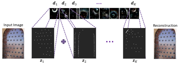
where are the vectorized 2D patches representing dictionary elements, and are the vectorized sparse maps corresponding to each of the dictionary elements (see Figure 1). The data term represents the image modelled by the sum of convolutions of the dictionary elements with their corresponding sparse maps, and controls the tradeoff between the sparsity of the feature maps and reconstruction error. The inequality constraint on the dictionary elements assumes Laplacian distributed coefficients, which ensures solving the problem at a proper scale for all elements since a larger value of would scale down the value of the corresponding . The above equation shows the objective function for a single image, and it can be easily extended to multiple images, where corresponding sparse maps are inferred for each image and all the images share the same dictionary elements.
3.1.1 CSC Subproblems
The objective in Eq. 1 is not jointly convex. However, using a fixed point approach (i.e.iteratively solving for one variable while keeping the other fixed) leads to two convex subproblems, which we refer to as the coding subproblem and the dictionary learning subproblem. For ease of notation, we represent the convolution operations by multiplication of Toeplitz matrices with the corresponding variables.
Coding Subproblem. We infer the sparse maps for a fixed set of dictionary elements as shown in Eq. 2.
| (2) |
Here, is of size and is a concatenation of the convolution matrices of the dictionary elements, and is a concatenation of the vectorized sparse maps.
Learning Subproblem. We learn the dictionary elements for a fixed set of sparse feature maps as shown in Eq. 3.
| (3) | ||||
Similar to above, is of size and is a concatenation of the sparse convolution matrices, is a concatenation of the dictionary elements, and projects the filter onto its spatial support.
The above two subproblems can be optimized iteratively using ADMM [10, 12], where each ADMM iteration requires solving a large linear system of size for each of the two variables and . Moreover, when applied to multiple images, solving the linear systems for the coding subproblem can be done separably, but should be done jointly for the learning subproblem, since all images share the same dictionary elements (see Section 4.2 for more details on complexity analysis).
3.2 CSC Dual Optimization
In this section, we show our approach to solving the CSC subproblems in the dual domain. Formulating the problems in the dual domain reduces the number of parameters involved in the linear systems from to , which leads to faster convergence towards a feasible solution and thus better computational performance. Since the two subproblems are convex, the duality gap is zero and solving the dual problem is equivalent to solving the primal form. In addition, similar to [10], we also solve the convolutions efficiently in the Fourier domain as described below.
3.2.1 Coding Subproblem
To find the dual problem of Eq. 2, we first introduce a dummy variable with equality constraints to yield the following formulation
| (4) | ||||
The Lagrangian of this problem would be:
| (5) |
which results in the following dual optimization with dual variable :
| (6) |
Solving the minimizations over and and using the definition of the conjugate function to the norm, we get the dual problem of Eq. 2 as:
| (7) | ||||
Coding Dual Optimization. Now, we show how to solve the optimization problem in Eq. 7 using ADMM. ADMM generally solves convex optimization problems by breaking the original problem into easier subproblems that are solved iteratively. To apply ADMM here, we introduce an additional variable , which allows us to write the problem in the general ADMM form as shown in Eq. 8. Since the dual solution to a dual problem is the primal solution for convex problems, the Lagrange multiplier involved in the ADMM update step is the sparse map vector in Eq. 2.
| (8) | ||||
Here, is the indicator function defined on the convex set of constraints . Deriving the augmented Lagrangian of the problem and solving for the ADMM update steps [29] yields the following iterative solutions to the dual problem with representing the iteration number.
| (9) | ||||
The parameter denotes the step size for the ADMM iterations, and represents the projection operator onto the set . The linear systems shown above do not require expensive matrix inversion or multiplication as they are transformed to elementwise divisions and multiplications when solved in the Fourier domain. This is possible because ignoring the boundary effects leads to a circulant structure for the convolution matrices, and thus they can be expressed by their base sample as follows:
| (10) |
where denotes the Discrete Fourier Transform (DFT) of , is the DFT matrix independent of , and is the Hermitian transpose.
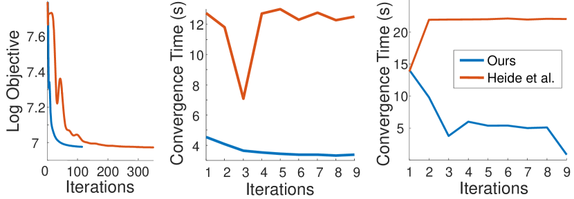
In our formulation, the -update step requires solving a linear system of size . Heide et al. [12] however solve the problem in the primal domain in which the -update step involves solving a much larger system of size . Clearly, our solution in the dual domain will lead to faster ADMM convergence. Figure 2-left shows the coding subproblem convergence of our approach and that of Heide et al.Our dual formulation leads to convergence within less iterations compared to the primal domain. In addition, our approach achieves a lower objective in general at any feasible number of iterations.
3.2.2 Learning Subproblem
To find a solution for Eq. 3, we minimize the Lagrangian of the problem (see Eq. 11) assuming optimal values for the Lagrange multipliers . This results in the optimization problem shown in Eq. 12.
| (11) |
| (12) |
To find the dual problem of Eq. 12, we follow a similar approach to the inference subproblem by introducing a dummy variable with equality constraints such that . Deriving the Lagrangian of the problem and minimizing over the primal variables yields the dual problem shown in 13.
| (13) |
Learning Dual Optimization. The optimization problem in Eq. 13 has a closed form solutionas shown in Eq. 14.
| (14) |
Given the optimal value for the dual variable , we can compute the optimal value for the primal variable as follows:
| (15) |
To find the optimal values for the Lagrange multipliers , we need to assure that the KKT conditions are satisfied. At optimal , the solution to the primal problem in Eq. 3 and its Lagrangian are equal. Thus, we end up with the below iterative update step for .
| (16) |
The learning subproblem is then solved iteratively by alternating between updating as per Eqs. 14,15 and updating as per Eq. 16 until convergence is achieved.
We use conjugate gradient to solve the system involved in the -update step by applying the heavy convolution matrix multiplications in the Fourier domain. The computation cost for solving this system decreases with ADMM iterations, since we employ a warm start where we initialize with the solution from the previous iteration. Figure 2-right shows the decreasing computation time of the learning subproblem of our approach.
For more details on the derivations of the coding and learning subproblems as well as the solutions to the equations in the Fourier domain, you may refer to the supplementary material.
3.2.3 Coordinate Descent
Now that we derived a solution to the two subproblems, we can use coordinate descent to solve the joint objective in Eq. 1 by alternating between the solutions for and . The full algorithm for the CSC problem is shown in Alg. 1.
The coordinate descent algorithm above guarantees a monotonically decreasing joint objective. We keep iterating until convergence is reached, i.e.when the change in the objective value, or the solution for the optimization variables and reaches a user-defined threshold . For solving the coding and learning subproblems, we also run the algorithms until convergence.
3.3 Higher Order Tensor CSC
Higher order tensor CSC [27] allows convolutional sparse coding over higher dimensional input such as a set of 3D input images as well as 4D videos. Similar to before, given the input data, we seek to reconstruct using patches convolved with sparse maps. In this formulation, each of the patches is of the same order of dimensionality as the input data with the possibility of a smaller spatial support. In addition, TCSC allows high dimensional correlation among features in the data. In this sense, unlike traditional CSC in which a separate sparse code is learned for separate features, the sparse maps in TCSC are shared along one of the dimensions such as the color channels for images/videos. The reader may be referred to the paper by Bibi et al. [27] for more details of the derivations for TCSC. Below we give our approach to solving the TCSC coding and learning subproblems in the dual domain.
The dictionary elements are represented by a tensor where represents the correlated input dimension (usually referring to data features/channels), is the number of elements, and are the uncorrelated dimensions (i.e. representing the spatial dimensions for images, and representing the spatial and time dimensions for videos). In our dual formulation, we perform circulant tensor unfolding [27] resulting in a block circulant dictionary matrix of size where . Thus, each of the convolution matrices is now of size where .
4 Results
In this section, we give an overview of the implementation details and the parameters selected for our dual CSC solver. We also show the complexity analysis and convergence of our approach compared to [12], the current state-of-the-art CSC solver. Finally, we show results on 4D TCSC using color input images as well as 5D TCSC using colored videos.
4.1 Implementation Details
We implemented the algorithm in MATLAB using the Parallel Computing Toolbox and we ran the experiments on an Intel 3.1GHz processor machine. We used the code provided by [12] in the comparisons for regular CSC and by [27] in the comparisons to TCSC. We evaluate our approach on the fruit and city datasets formed of 10 images each, the house dataset containing 100 images, and basketball video from the OTB50 dataset selecting 10 frames similar to [27].
We apply contrast normalization to the images prior to learning the dictionaries for both gray scale and color images; thus, the figures show normalized patches. We show results by varying the sparsity coefficient , the number of dictionary elements , and the number of images . In our optimization, we choose a constant value of for the ADMM step size. We also initialize and with zeros for the first iteration of the learning subproblem, and with random values in the coding subproblem. Our results compare with Heide et al. [12] for regular CSC, as it is the fastest among the published methods discussed in the related work section, and with Bibi et al. [27] for TCSC as it is the only method that deals with higher order CSC.

4.2 Complexity Analysis
In this section, we analyze the per-iteration complexity of our approach compared to [12] and [27] with respect to each of the subproblems as shown in Table 1. In the equations below, corresponds to the product of the order of the uncorrelated dimensions (e.g. number of pixels for images), is the number of channels in the correlated input dimension, and is the number of conjugate gradient iterations within the learning subproblem. For regular CSC on high dimensional data, we assume that the problem is solved separately for each of the channels.
Coding Subproblem. In the coding subproblem, the complexity of our approach is similar to that of [12] for regular 2D CSC (). The computational complexity is dominated by solving the linear system by elementwise product and division operations in the Fourier domain. Although the two approaches are computationally similar here, it is important to note that the number of variables involved in solving the systems is much less in our approach. In practice, we observe that this also leads to faster convergence for the subproblem as shown in Figure 2. For higher order dimensional CSC (), our formulation is linear in the number of filters compared to a cubic cost for TCSC. In TCSC, the Sherman Morrison formula no longer applies and the computation is dominated by solving linear systems of size .
Learning Subproblem. Here, our approach solves the problem iteratively using conjugate gradient to solve the linear system. Thus, the computational cost lies in solving elementwise products and divisions, with the additional cost of applying the Fourier transforms to the variables. On the other hand, Heide et al. [12] and Bibi et al. [27] need to solve the subproblem by applying ADMM.
We observe that the performance of our dictionary learning approach improves by increasing the number of conjugate gradient iterations involved in solving the linear system. This number decreases after each inner iteration and its cost becomes negligible within 4-6 iterations due to the warm-start initialization of at each step as shown in Figure 2. On the other hand, Heide et al. [12] and Bibi et al. [27] incur the additional cost of solving the linear systems. Thus, our method has better scalability compared to the primal methods in which the linear systems solving step dominates as the number of images and filters increase (see section 4.4).
4.3 CSC Convergence
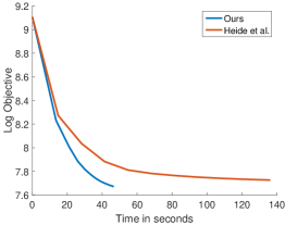
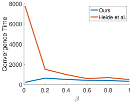
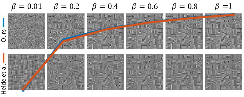
In this section, we analyse the convergence properties of our approach to regular convolutional sparse coding. In Figure 3, we plot the convergence of our method compared to the state of the art [12] on the city dataset for fixed and . We also show the progression of the learnt filters in correspondence with the curves. As shown in the figure, the two methods converge to the same solution. Figure 4a plots how the objective value decreases with time for each of the two methods using the same parameters as above. This shows that our method converges significantly faster than [12].
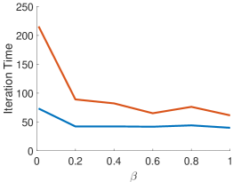
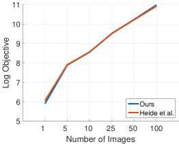
We also plot in Figure 5 the objective value as a function of the sparsity coefficient . The plot shows how increasing the sparsity coefficient results in an increase in the objective value, and more importantly, it verifies that our method converges to an objective value similar to that of [12] even though we reach a solution faster as shown in Figure 4c. Figure 5 also shows how the dictionary elements vary with .
4.4 Scalability
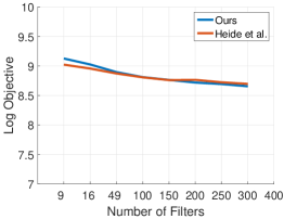
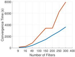
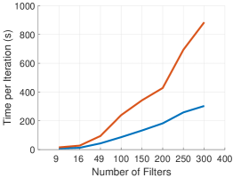
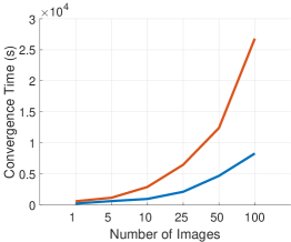
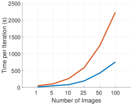
In this section, we analyze the scalability of the CSC problem with increasing number of filters and images. We compare our approach to Heide et. al. [12] in terms of the overall convergence time and average time per iteration for reaching the same final objective value. To ensure that the two problems achieve similar overall objective values, we make sure that each of the methods runs until convergence for both the coding and learning convex subproblems with the same initial point. Figure 6 shows that the computation time of each of the methods increases when the number of filters and images increases. It also shows a significant speedup (about 2.5x) for our approach over that of [12].
4.5 TCSC Results
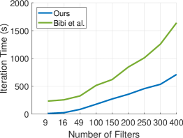
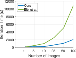
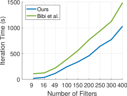
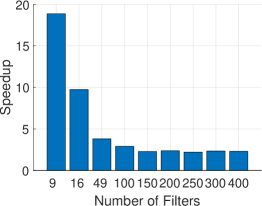
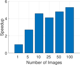
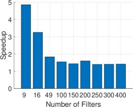
In this section, we show results for TCSC on color images and videos. We compare the performance of our dual formulation for TCSC with that of Bibi et al. [27]. Figures 7a and 7b show iteration time results on color images from the fruit and house datasets respectively with varying the number of filters and number of images. Correspondingly, we show the speedup acheived by our dual formulation for images and videos in Figure 8. As shown, our dual formulation achieves up to 20 times speed-up compared to the primal solution. We can observe higher speedups for smaller number of filters and we can also observe that the speedup is approximately constant as the number of images increases. This is inline with our complexity analysis in which we verified that Sherman Morrison formula is no longer applicable in the primal domain for TCSC, while parallelization is still applicable in the dual.
5 Conclusion and Future Work
We proposed our approach for solving the convolutional sparse coding problem by posing and solving each of its underlying convex subproblems in the dual domain. This results in a lower computational complexity than previous work. We can also easily extend our proposed solver to CSC problems of higher dimensional data. We demonstrated that tackling CSC in the dual domain results in up to 20 times speedup compared to the current state of the art. In future work, we would like to experiment with additional regularizers for CSC. We could make use of the structure of the input signal and map the regularizer over to the sparse maps to reflect this structure. For example, for images with a repetitive pattern, a nuclear norm can be added as a regularizer, which is equivalent to making the sparse maps low rank.
References
- [1] Elad, M., Aharon, M.: Image denoising via sparse and redundant representations over learned dictionaries. IEEE Transactions on Image processing 15(12) (2006) 3736–3745
- [2] Aharon, M., Elad, M., Bruckstein, A.M.: On the uniqueness of overcomplete dictionaries, and a practical way to retrieve them. Linear algebra and its applications 416(1) (2006) 48–67
- [3] Couzinie-Devy, F., Mairal, J., Bach, F., Ponce, J.: Dictionary learning for deblurring and digital zoom. arXiv preprint arXiv:1110.0957 (2011)
- [4] Yang, J., Wright, J., Huang, T., Ma, Y.: Image super-resolution as sparse representation of raw image patches. In: Computer Vision and Pattern Recognition, 2008. CVPR 2008. IEEE Conference on, IEEE (2008) 1–8
- [5] Gu, S., Zuo, W., Xie, Q., Meng, D., Feng, X., Zhang, L.: Convolutional sparse coding for image super-resolution. ICCV (2015)
- [6] Zhu, Y., Lucey, S.: Convolutional sparse coding for trajectory reconstruction. PAMI (2015)
- [7] Heide, F., Xiao, L., Kolb, A., Hullin, M.B., Heidrich, W.: Imaging in scattering media using correlation image sensors and sparse convolutional coding. Optics express (2014)
- [8] Zhang, T., Bibi, A., Ghanem, B.: In Defense of Sparse Tracking: Circulant Sparse Tracker. CVPR (2016)
- [9] Krizhevsky, A., Sutskever, I., Hinton, G.E.: Imagenet classification with deep convolutional neural networks. In: Advances in neural information processing systems. (2012)
- [10] Bristow, H., Eriksson, A., Lucey, S.: Fast Convolutional Sparse Coding. CVPR (2013)
- [11] Kong, B., Fowlkes, C.C.: Fast Convolutional Sparse Coding. Tech. Rep. UCI (2014)
- [12] Heide, F., Heidrich, W., Wetzstein, G.: Fast and Flexible Convolutional Sparse Coding. CVPR (2015)
- [13] Zeiler, M.D., Krishnan, D., Taylor, G.W., Fergus, R.: Deconvolutional networks. In: CVPR. (2010)
- [14] Olshausen, B.A., Field, D.J.: Sparse coding with an overcomplete basis set: A strategy employed by v1? Vision research 37(23) (1997) 3311–3325
- [15] Lee, H., Battle, A., Raina, R., Ng, A.Y.: Efficient sparse coding algorithms. In: Advances in neural information processing systems. (2006) 801–808
- [16] Mairal, J., Bach, F., Ponce, J., Sapiro, G.: Online dictionary learning for sparse coding. In: Proceedings of the 26th annual international conference on machine learning, ACM (2009) 689–696
- [17] Mairal, J., Ponce, J., Sapiro, G., Zisserman, A., Bach, F.R.: Supervised dictionary learning. In: Advances in neural information processing systems. (2009) 1033–1040
- [18] Kavukcuoglu, K., Sermanet, P., Boureau, Y.L., Gregor, K., Mathieu, M., Cun, Y.L.: Learning convolutional feature hierarchies for visual recognition. In: Advances in neural information processing systems. (2010) 1090–1098
- [19] Li, Y., Osher, S.: Coordinate descent optimization for ℓ 1 minimization with application to compressed sensing; a greedy algorithm. Inverse Probl. Imaging 3(3) (2009) 487–503
- [20] Yang, J., Yu, K., Huang, T.: Supervised translation-invariant sparse coding. In: Computer Vision and Pattern Recognition (CVPR), 2010 IEEE Conference on, IEEE (2010) 3517–3524
- [21] Šorel, M., Šroubek, F.: Fast convolutional sparse coding using matrix inversion lemma. Digital Signal Processing 55 (2016) 44–51
- [22] Bristow, H., Lucey, S.: Optimization Methods for Convolutional Sparse Coding. arXiv Prepr. arXiv1406.2407v1 (2014)
- [23] Zhong, W., Kwok, J.T.Y.: Fast stochastic alternating direction method of multipliers. In: ICML. (2014) 46–54
- [24] Wang, Y., Yao, Q., Kwok, J.T., Ni, L.M.: Online convolutional sparse coding. CoRR abs/1706.06972 (2017)
- [25] Wohlberg, B.: Boundary handling for convolutional sparse representations. In: Image Processing (ICIP), 2016 IEEE International Conference on, IEEE (2016) 1833–1837
- [26] Wohlberg, B.: Convolutional sparse representation of color images. In: Image Analysis and Interpretation (SSIAI), 2016 IEEE Southwest Symposium on, IEEE (2016) 57–60
- [27] Bibi, A., Ghanem, B.: High order tensor formulation for convolutional sparse coding. In: Proceedings of the IEEE Conference on Computer Vision and Pattern Recognition. (2017) 1772–1780
- [28] Choudhury, B., Swanson, R., Heide, F., Wetzstein, G., Heidrich, W.: Consensus convolutional sparse coding. In: Proceedings of the IEEE Conference on Computer Vision and Pattern Recognition. (2017) 4280–4288
- [29] Boyd, S., Parikh, N., Chu, E., Peleato, B., Eckstein, J.: Distributed optimization and statistical learning via the alternating direction method of multipliers. (2011)