Axion dark matter and the Lattice

Abstract

First I will review the QCD theta problem and the Peccei-Quinn solution, with its new particle, the axion. I will review the possibility of the axion as dark matter. If PQ symmetry was restored at some point in the hot early Universe, it should be possible to make a definite prediction for the axion mass if it constitutes the Dark Matter. I will describe progress on one issue needed to make this prediction – the dynamics of axionic string-wall networks and how they produce axions. Then I will discuss the sensitivity of the calculation to the high temperature QCD topological susceptibility. My emphasis is on what temperature range is important, and what level of precision is needed.

1 Overview

The axion Peccei:1977hh ; Peccei:1977ur ; Weinberg:1977ma ; Wilczek:1977pj is a proposed particle, the angular excitation of a new “Peccei-Quinn” (PQ) field $\varphi$ that would solve the strong CP problem tHooft:1976 ; Jackiw:1976pf ; Callan:1979bg and which is also a very interesting dark matter candidate Preskill:1982cy ; Abbott:1982af ; Dine:1982ah , thereby solving two puzzles with one mechanism. That’s why I think it well motivated to study the axion as a dark matter candidate. The axion model has one undetermined parameter, the vacuum value of $\varphi$, $f_{a}$; the axion mass $m_{a}$ scales as $f_{a}^{-1}$. The value of $f_{a}$ also plays a role in determining the amount of axion dark matter produced in the early Universe. So do some nontrivial dynamics which we will explain in detail below. If we can understand the nontrivial dynamics of the axion field during cosmology, that lets us find a fixed relation between $f_{a}$ and the (measured) dark matter abundance. It therefore allows a clean determination of the axion mass, under some simple assumptions. This is valuable in the experimental search for the axion and it motivates us to solve the cosmological axion dynamics.

Supposing we make the following assumptions:

• The axion exists.

• The axion field starts out “random” (in a sense we will define precisely below) either during or shortly after inflation (or whatever physics featured in the Universe at very high energy density).

• Gravity and the Universe’s energy budget followed the “standard” picture (General Relativity and the known Standard Model species dominating the energy density) at temperatures $T<2$ GeV.

• Axions make up all of the observed dark matter.

Then, as I will explain, we have enough information to determine the axion mass. But to do so we will need to solve two problems:

1. We need to know the temperature dependence of the QCD topological susceptibility at temperatures between 540 and 1150 MeV.

2. We need to control the axion field dynamics during this temperature range, to solve for the efficiency of axion production.

The session following this talk addresses item 1 and the remainder of this talk will lay out the groundwork more completely and will then address item 2.

2 Strong CP problem and the axion

Let me refresh your memories on the strong CP problem. There are two gauge-invariant dimension-4 scalars which can enter the gauge-field part of the QCD Lagrangian:

$$\mathcal{L}=\frac{1}{2g^{2}}\,\mathrm{Tr}\,G_{\mu\nu}G_{\mu\nu}+\frac{\Theta}{32\pi^{2}}\,\mathrm{Tr}\,\epsilon_{\mu\nu\alpha\beta}G^{\mu\nu}G^{\alpha\beta}\,.$$ (1)

The latter term is P and T odd because it contains the antisymmetric tensor $\epsilon_{\mu\nu\alpha\beta}$. The operator which $\Theta$ multiplies is the topological density and it integrates to the instanton number. Its zero-momentum two-point function defines the topological susceptibility,

$$\chi(T)\equiv\left\langle\int d^{4}x\frac{1}{32\pi^{2}}\epsilon_{\mu\nu\alpha\beta}\,\mathrm{Tr}\,G_{\mu\nu}G_{\alpha\beta}(x)\;\frac{1}{32\pi^{2}}\epsilon_{\sigma\rho\kappa\zeta}\,\mathrm{Tr}\,G_{\sigma\rho}G_{\kappa\zeta}(0)\right\rangle_{T}\,,$$ (2)

$\langle\ldots\rangle_{T}$ means the expectation value in the thermal ensemble at temperature $T$.

Such a term is strongly constrained by the absence of a measured neutron electric dipole moment. The experimental limit of Baker:2006ts

$$|d_{n,\mathrm{meas}}|<2.9\times 10^{-26}\;e\,\mathrm{cm}$$ (3)

contradicts the lattice results for the dipole moment from $\Theta$ Guo:2015tla

$$d_{n}=-3.8\times 10^{-16}\;e\,\mathrm{cm}\times\Theta$$ (4)

unless $|\Theta|<10^{-10}$. At this conference we saw new results for the lattice $\Theta$-dependent dipole moment which show that the above result may be too high and its error bar was certainly underestimated (see Abramczyk:2017oxr ; Liu:2017man and these proceedings). However it is clear that the absence of a neutron electric dipole moment places an extremely tight constraint on $\Theta$.

This is hard to understand because we know P and T are not fundamental symmetries; and any physics at a high scale which violates them generically gives rise to a $\Theta$ which does not decrease as we move to lower scales. For instance, consider a very heavy Dirac quark species $Q$, with Lagrangian

$$\mathcal{L}_{Q}=\bar{Q}\not{D}Q+\left(m\bar{Q}P_{\scriptscriptstyle L}Q+m^{*}\bar{Q}P_{\scriptscriptstyle R}Q\right)\,.$$ (5)

Note that $m$ can be complex, since $(\bar{Q}P_{\scriptscriptstyle L}Q)^{\dagger}=\bar{Q}P_{\scriptscriptstyle R}Q$. But an imaginary part is T and P odd, since the role of left and right projector, $P_{\scriptscriptstyle L}$ and $P_{\scriptscriptstyle R}$, switch under parity and because T is antiunitary. We can remove this mass through a chiral rotation of $Q$,

$$Q\to(e^{-i\,\mathrm{arg}\,m/2}P_{\scriptscriptstyle L}+e^{-i\,\mathrm{arg}\,m/2}P_{\scriptscriptstyle R})Q\,,$$ (6)

at the cost of reintroducing it, via the Fujikawa mechanism Fujikawa:1979ay ; Fujikawa:1980eg , as a shift in the value of $\Theta$,

$$\Theta\to\Theta-\mathrm{arg}\,m\,.$$ (7)

Therefore even a very heavy quark can influence the P and T symmetry properties of low energy QCD.

But what if there is a symmetry forbidding the mass term for this quark? For instance, suppose $P_{\scriptscriptstyle L}Q$ is charge 1 and $P_{\scriptscriptstyle R}Q$ is charge-0 under some global U(1) symmetry? Then the mass term breaks this symmetry, but a complex scalar $\varphi$ with charge 1 under the symmetry could induce a mass via a Yukawa interaction and a vacuum value. The possible Lagrangian terms for such a scalar are

$$\mathcal{L}_{\varphi}=\partial_{\mu}\varphi^{*}\partial_{\mu}\varphi+\frac{m^{2}}{8f_{a}^{2}}\left(f_{a}^{2}-2\varphi^{*}\varphi\right)^{2}+\Big{(}y\varphi\bar{Q}P_{\scriptscriptstyle R}Q+y^{*}\varphi^{*}\bar{Q}P_{\scriptscriptstyle L}Q\Big{)}\,.$$ (8)

The combination $y\varphi$ plays the role of $m^{*}$ in the previous case. But now $\,\mathrm{Arg}\,\varphi$ is a dynamical quantity. We will be interested in temperatures around 1 GeV and $\varphi$ varying on scales of the Hubble scale at that time – tens of meters! Therefore from the point of view of QCD we can take $\varphi$ to be space-independent, and perform an $\,\mathrm{Arg}\,\varphi$ dependent rotation on $Q$, making the theta term

$$\Theta\to\Theta+\,\mathrm{Arg}\,\varphi\,.$$ (9)

Here we have absorbed the phase in $y$ into a phase redefinition of $\varphi$. We can also absorb $\Theta$ in the same way, so that $\,\mathrm{Arg}\,\varphi$ alone plays the role of $\Theta$-angle. For notational compactness we will henceforth write $\varphi=ve^{i\theta_{\mathrm{a}}}$, with $\theta_{\mathrm{a}}=\,\mathrm{Arg}\,\varphi$. This specific way of coupling QCD topology to a complex scalar is called the KSVZ axion Kim:1979if ; Shifman:1979if . There are other mechanisms but the low-energy phenomenology is essentially identical and this mechanism is particularly clear to understand.

From the point of view of QCD, the $\Theta$-angle is replaced by a possibly spacetime-varying dynamical field $\theta_{\mathrm{a}}$. What about from the point of view of the field $\varphi$? Since we want physics on the meter length scale, we can integrate out QCD, leading to an effective potential:

$$V_{\mathrm{eff}}(\theta_{\mathrm{a}}) = -\frac{T}{\Omega}\ln\int\mathcal{D}(A_{\mu}\bar{\psi}\psi)\,\mathrm{Det}\,(\not{D}{+}m)e^{-\int d^{4}x\frac{1}{2g^{2}}\,\mathrm{Tr}\,G_{\mu\nu}G_{\mu\nu}}\times e^{i\theta_{\mathrm{a}}\int d^{4}x\frac{1}{32\pi^{2}}\epsilon_{\mu\nu\alpha\beta}\,\mathrm{Tr}\,G_{\mu\nu}G_{\alpha\beta}}$$ (10)

$$\simeq \chi(T)(1-\cos\,\theta_{\mathrm{a}})\,,$$

with $\Omega$ the volume of space included in the path integration. In the second line we have made a dilute instanton approximation, which is that the integration exponentiates over the two-point function of the topological density, controlled by the topological susceptibility $\chi(T)$ introduced already in Eq. (2). This is not a good approximation for large $\theta_{\mathrm{a}}$ and low temperatures diCortona:2015ldu , but it works well when instantons are dilute, which is true for $T>500\>\mathrm{MeV}$, and for small values of $\theta_{\mathrm{a}}$, which will be all we encounter below this temperature. So we can actually use this approximation all the time. Independent of this approximation, it is easy to see that the effective potential is smallest (the $\theta_{\mathrm{a}}$ choice is most energetically favored) for $\theta_{\mathrm{a}}=0$ and therefore when P and T symmetry are restored. Note that $\theta_{\mathrm{a}}$ only enters as the coefficient in a complex phase, in an otherwise real and positive integral. The integral is maximized, and the free energy minimized, if the phase is always unity. Any nonzero value of $\theta_{\mathrm{a}}$ gives rise to phase cancellations and therefore suppresses the partition function, raising the free energy.

Although we derived it in Euclidean space, we can also use this effective potential in Minkowski space to study the spacetime evolution of the $\varphi$ field. In summary, the Minkowski effective Lagrangian for the $\varphi$ field is

$$-\mathcal{L}_{\varphi}=\partial_{\mu}\varphi^{*}\partial^{\mu}\varphi+\frac{m^{2}}{8f_{a}^{2}}\left(f_{a}^{2}-2\varphi^{*}\varphi\right)^{2}+\chi(T)(1-\cos\theta_{\mathrm{a}})\,.$$ (11)

We will use this to determine the dynamics of the field in the next sections.

3 Axion in Cosmology

Let us see what happens to the axion field during cosmological evolution.

3.1 Value of susceptibility

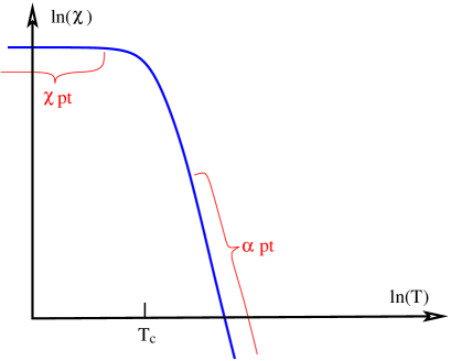
Figure 1: Cartoon of what we know about the topological susceptibility as a function of temperature (log-log plot). At low temperatures, chiral perturbation theory gives us the zero-temperature limit and small-temperature behavior. At large temperatures, perturbation theory predicts a power-law falloff with a power near 8.

The form of Eq. (11) makes it clear that, in order to study the axion’s role in cosmology, we are going to need to know the temperature dependence of the topological susceptibility $\chi(T)$. It does not yet tell us what temperature range will be interesting. Figure 1 shows our knowledge at the cartoon level. At low temperature or vacuum, chiral perturbation theory works and diCortona:2015ldu

$$\chi(T\to 0)\simeq\frac{m_{u}m_{d}}{(m_{u}+m_{d})^{2}}m_{\pi}^{2}f_{\pi}^{2}\simeq(76\>\mathrm{MeV})^{4}\,.$$ (12)

At high temperatures we have conventional perturbation theory, which forecasts Gross:1980br that $\chi(T)\propto T^{-7-N_{f}/3}$. However the exact coefficient is sensitive to the physics of electric screening and is not known accurately. This is why we need lattice results for this quantity! Recently there have been several Berkowitz:2015aua ; Borsanyi:2015cka ; Petreczky:2016vrs ; Taniguchi:2016tjc ; Burger:2017xkz ; Frison:2016vuc ; Borsanyi:2016ksw , which give generally compatible results but generally at temperatures below 600 MeV (or in the quenched approximation). It takes new techniques to reach higher temperatures, and only one recent paper Borsanyi:2016ksw achieves this, reaching temperatures of 1500 MeV. Also, one group Bonati:2015vqz ; Bonati:2016imp finds results which are discrepant with the others, indicating that the matter is not yet settled. Here we will assume that the results of Borsanyi:2016ksw are correct. This may well be the case, but we leave the discussion of the relative merits of these approaches and results to the panel, who have more expertise. Needless to say it would be valuable to know definitively that $\chi(T)$ is well determined.

3.2 Space-uniform axion field

So let’s assume for now that we know $\chi(T)$. For simplicity let us also assume that the axion takes the same value everywhere in space, $\theta_{\mathrm{a}}(x,t)=\theta_{\mathrm{a}}(t)$. It is simplest to work in terms of conformal time, so the metric is $g_{\mu\nu}=a^{2}(t)\eta_{\mu\nu}$ with $a$ the scale factor. (Later we will use $a$ to represent the lattice spacing. This is actually the same thing, since we will work in comoving coordinates; the lattice spacing is proportional to the scale factor and we may as well use a proportionality of 1.) In the radiation era $a(t)\propto t$ and $T\propto t^{-1}$. The radial component of $\varphi=ve^{i\theta_{\mathrm{a}}}$ is inactive, $v=f_{a}$, and the angular part obeys

$$\mathcal{L} = f_{a}^{2}t^{2}\left(\frac{1}{2}(\partial_{t}\theta_{\mathrm{a}})^{2}+t^{2}\tilde{\chi}(t^{-1})(1-\cos\theta_{\mathrm{a}})\right)\,,$$ (13)

$$\partial_{t}^{2}\theta_{\mathrm{a}}+\frac{2}{t}\partial_{t}\theta_{\mathrm{a}} = -t^{2}\tilde{\chi}(t^{-1})\sin\theta_{\mathrm{a}}\,,$$ (14)

where $\tilde{\chi}(t^{-1})$ is a rescaled form of the susceptibility. This leads to damped, anharmonic oscillations. The oscillations start roughly at the time $t_{*}$ when $t_{*}^{2}\tilde{\chi}(t_{*}^{-1})=t_{*}^{-2}$, or in physical units, when $m_{a}\equiv\sqrt{\chi(T)/f_{a}^{2}}$ obeys $m_{a}t_{*}=1$ or equivalently $m_{a}/H=1$ with $H$ the Hubble scale. After this time the oscillations accelerate as $t^{2}\tilde{\chi}$ increases, and they damp away. The damping arises both from the $2\partial_{t}\theta_{\mathrm{a}}/t$ term (Hubble drag) and from the time variation of the susceptibility. After several oscillations the axion particle number becomes an approximate adiabatic invariant, with number density parametrically of form $(t_{*}/t)^{2}(f_{a}^{2}/t_{*})$. We see that the number density is quadratic in $f_{a}$, while the axion mass is $m_{a}\propto f_{a}^{-1}$. Because $\chi(T)$ is a very strong function of temperature, $t_{*}$ depends only weakly on $f_{a}$, and so the generated axion energy density is almost linear in $f_{a}$.

Therefore, the larger the value of $f_{a}$, the larger the produced axion abundance. However the axion abundance also depends on the unknown initial angle $\theta_{\mathrm{a}}(t=0)$. Therefore the dark matter density depends on two variables and it is impossible to make a clean prediction for the value of $f_{a}$. We can make a baseline prediction, however, by averaging over the value of the starting angle $\theta_{\mathrm{a}}(t=0)$. Doing so, one finds the axion mass should be $32\,\mu\mathrm{eV}$, and $t_{*}$ corresponds to a temperature of $T_{*}=1.6\,\mathrm{GeV}$.

3.3 Space-random axion field

It is far more likely that the Universe started out with a spatially random value for $\theta_{\mathrm{a}}$, with no correlations on scales longer than the Hubble scale. Arguments for this picture are presented in Visinelli:2014twa and are summarized as follows:

• It is likely that inflation occurs with a high scale, $H^{2}>f_{a}^{2}/60$. In this case, over 60 efoldings of inflation, quantum fluctuations stretched (squeezed) by inflation into classical fluctuations would randomize the value of the axion field over the course of inflation. The observation of cosmological tensor modes would more-or-less settle this issue.

• After inflation, the Universe reheats to a temperature which can be as high as $T_{\mathrm{rh}}\sim 0.1\sqrt{Hm_{\mathrm{pl}}}$. Even if $H\ll f_{a}$, if the reheat temperature is $T_{\mathrm{rh}}>f_{a}$, there would be thermal symmetry restoration for $\varphi$. Then when the temperature falls below this scale, $\varphi$ would independently take on a vacuum value at different points in space, which would be uncorrelated.

• The case where inflation and reheating are both low-scale is actually tightly constrained by the absence of observed isocurvature fluctuations (different fluctuations in $\theta_{\mathrm{a}}$ than in the radiation temperature), which require roughly $H<10^{-5}f_{a}$. Most inflation model-builders would consider this rather unlikely.

I emphasize that we do not know that $\theta_{\mathrm{a}}$ was randomized in the early Universe (assuming the axion exists). But it appears likely, and it motivates studying the consequences. I will also assume that the axion makes up all of the dark matter in the universe, so we may equate the final axion matter density with the dark matter density, which is known to obey $\rho_{\mathrm{dm}}/s=0.39\>\mathrm{eV}$ with $s$ the entropy density Ade:2015xua .

The space-inhomogeneous case is much more complicated than the space-homogeneous case. Nevertheless, in the remainder of the presentation I will show how to solve it.

4 Axion string/wall network

The $\varphi$ field varies with amplitude of order $f_{a}\sim 10^{11}\,\mathrm{GeV}$ over a length scale controlled by $H\sim T^{2}/m_{\mathrm{pl}}\sim 10^{-18}\,\mathrm{GeV}$. This huge hierarchy makes the dynamics those of a classical field to extremely high accuracy. The Lagrangian Eq. (11) (times $t^{2}$ to account for Hubble expansion) and resulting classical equations of motion are easy to put on the lattice and solve as a function of time, from random initial conditions. In broad brushstrokes, our approach is to do just this, evolving the system until only small fluctuations in $\theta_{\mathrm{a}}$ remain and their evolution has become adiabatic. Then we integrate the associated axion number,

$$n_{\mathrm{ax}}=\int\frac{d^{3}p}{(2\pi)^{3}}f(p)=\int\frac{d^{3}p}{(2\pi)^{3}}\frac{(p^{2}+m_{a}^{2})\varphi^{*}\varphi(p)+\dot{\varphi}^{*}\dot{\varphi}}{\sqrt{p^{2}+m_{a}^{2}}}$$ (15)

and compare it to the result of the angle-averaged misalignment baseline.

In fact such a simulation is not sufficient, because of the large hierarchy in Eq. (11) between the mass scale $m\sim 10^{11}\,\mathrm{GeV}$ of radial excitations and the mass scale $m_{a}=\sqrt{\chi(T)}/f_{a}\sim H\sim 10^{-18}\,\mathrm{GeV}$ of angular fluctuations. The simulations have to take place at the $m_{a}$ scale, which means that the radial-mass scale cannot be resolved. Naively this should not matter, as radial excitations should decouple. But it does matter, because the theory contains topological string defects which play a role in the dynamics, and the string tension depends logarithmically on the ratio $m/m_{a}$. Let’s explain this in a little more detail.

4.1 String defects

First note that $\theta_{\mathrm{a}}$ is only defined modulo $2\pi$. Therefore in traversing a circle, $\theta_{\mathrm{a}}$ might return to its starting value, but it might only return modulo $2\pi$, that is, $\oint\partial_{i}\theta_{\mathrm{a}}dx^{i}=2\pi N$. The integer $N$ is a winding number which counts a “flux” of string defects through the circle. If we deform a loop, $N$ can only change when the loop passes through a singularity in the $\theta_{\mathrm{a}}$ field. The locus of these singularities defines the axionic cosmic string.

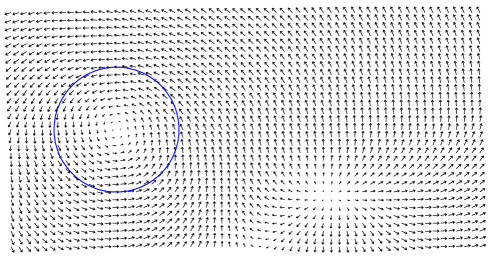
Figure 2: A 2D slice of a simulation, with the complex field $\varphi$ represented by a field of arrows with a length and direction. Going around the blue circle, the arrow direction winds by $2\pi$. The associated string defect is at the center of the circle; another string defect is farther down and to the right.

We illustrate the idea with Figure 2, which shows a 2D slice out of a simulation, representing the complex field as a field of arrows with length and direction. The field direction has singularities where the arrows have zero length; going around the singularity, the direction of $\varphi$ revolves by $\pm 2\pi$. The singular point extends in 3D into a line where the field has zero value; any loop circling this line will have the direction of $\varphi$ revolve by $\pm 2\pi$ as the one circles around the string.

Such a defect – essentially a vortex in the $\varphi$ field – is called an axionic cosmic string, and it is topologically stable; no local changes to the value of $\varphi$ can cause it to disappear. If PQ symmetry is restored in the early Universe, then $\theta_{\mathrm{a}}$ starts out uncorrelated at widely separated points and will generically begin with a dense network of these strings (the Kibble mechanism for string production Kibble:1976sj ). The strings evolve, straightening out, chopping off loops, and otherwise reducing their density, arriving at a scaling solution Albrecht:1984xv where the length of string per unit volume scales with time t as $t^{-2}$. They may play a dominant role in establishing axion production in the scenario under discussion Davis:1986xc .

Let us analyze the structure of a string in a little more detail. Consider a straight string along the $z$ axis; in polar $(z,r,\phi)$ coordinates the string equations of motion are solved by $\sqrt{2}\varphi=v(r)f_{a}e^{i\phi}$, with $v(r)\simeq 1$ for all $r\gg 1/m$; so $\theta_{\mathrm{a}}=\phi$ (up to a constant which we can remove by our choice of $x$-axis). The string’s energy is dominated by the gradient energy due to the space variation of $\theta_{\mathrm{a}}$:

$$T_{\mathrm{str}} = \frac{\mbox{Energy}}{\mbox{length}}=\int r\,dr\,d\phi\left(V(\varphi^{*}\varphi)+\frac{1}{2}\nabla\varphi^{*}\nabla\varphi\right)$$ (16)

$$\simeq \pi\int r\,dr\left(\frac{\partial_{\phi}\varphi^{*}}{r}\;\frac{\partial_{\phi}\varphi}{r}\right)\simeq\pi\int^{H^{-1}}_{1/m}r\,dr\;\frac{f_{a}^{2}}{r^{2}}=\pi f_{a}^{2}\ln(m/H)\equiv\pi f_{a}^{2}\kappa\,,$$ (17)

where the integral over $r$ is cut off at small $r$ by the scale where $v(r)\neq 1$ (the string core), and at large distances by the scale where the string is not alone in the Universe but its field is modified by other strings or effects; this should be the larger of $H$ and $m_{a}$. We define $\kappa=\ln(m/H)$ as the log of this scale ratio. Now $m$ is at most $f_{a}\sim 10^{11}\,\mathrm{GeV}$, and to ensure that the radial particles decay by the scale of 1 GeV we need $m>10^{3}\,\mathrm{GeV}$. Therefore $\kappa\in[48,67]$.

This logarithm, $\kappa$, controls several aspects of the strings’ dynamics. It controls the string tension, as we just saw. More relevant, while the string tension is $\pi\kappa f_{a}^{2}$, the string’s interactions with the long-range $\varphi$ field scale as $f_{a}^{2}$ without the $\kappa$ factor. Therefore the string’s long-range interactions become less important, relative to the string evolution under tension, as $\kappa$ gets larger. The long-range interactions are responsible for energy radiation from the strings, as well as for long-range, often attractive, interactions between strings. Since these effects tend to deplete and straighten out the string network, the large-$\kappa$ theory will have denser, kinkier strings. Indeed, in the large $\kappa$ limit the string behavior should go over to that of local (Nambu-Goto) strings Dabholkar:1989ju . Unfortunately, a numerical implementation must resolve the length scale $m$, $ma\leq 1$, and cannot exceed $m/H\sim 1000$; numerical studies of the scalar field system have $\kappa<7$, nearly an order of magnitude too small.

4.2 Wall defects

Besides the strings, there are also wall defects. These occur late in the simulation when $m_{a}\gg H$. The potential term $\chi(T)(1-\cos\theta_{\mathrm{a}})$ then forces $\theta_{\mathrm{a}}\simeq 0$ nearly everywhere – modulo $2\pi$. But suppose some region has $\theta_{\mathrm{a}}\simeq 0$ and another has $\theta_{\mathrm{a}}\simeq 2\pi$. There must be some 2D surface between them with $\theta_{\mathrm{a}}\simeq\pi$. This is a wall defect. The region near the defect where $\theta_{\mathrm{a}}$ differs significantly away from its minimum has thickness $\ell\sim 1/m_{a}$, which is easily resolved on the lattice. The surface tension of such a surface turns out to be $8m_{a}f_{a}^{2}$. A 2D slice of a configuration, illustrating such a domain wall attached to a string, is shown in Figure 3.

Figure 3: A 2D slice of a simulation, this time with a string (lower left) attached to a domain wall which extends near the bottom, off the right edge.

These wall defects are not a problem to simulate. But they play an important role in the dynamics. Every string has $\theta_{\mathrm{a}}$ take every value $[0,2\pi]$ as one goes around the string. That includes $\theta_{\mathrm{a}}=\pi$. Therefore every string is attached to a domain wall. When $m_{a}$ becomes $m_{a}\gg\kappa H$, the force from the domain wall tension becomes large enough to pull around the strings, leading to the collapse of the string network and the annihilation of all strings. It is only after this network collapse that one can speak about axion number. Because of the factor $\kappa$ in the needed tension, a large-$\kappa$ simulation will feature a more persistent string network.

One final problem for scalar-only simulations, pointed out in axion1 , is that the domain walls actually lose even their metastability as soon as $m_{a}^{2}/m^{2}>1/39$. This drives up the required size of simulations so that large $m$ can be achieved.

5 Simulating high-tension strings

We see from the previous section that simulations of the $\varphi$ field alone are not reliable. Although one can make the scale $m$ very heavy compared to $H,m_{a}$, the string tension depends logarithmically on this scale, and is nearly a factor of 10 too small. This profoundly affects the dynamics of the string network, and therefore renders the results unreliable. We need a method to simulate high-tension strings coupled to $\theta_{\mathrm{a}}$. We found such a method in axion3 and present it here.

5.1 Effective theory

We are interested in the large-scale structure of string networks and the infrared behavior of any (pseudo)Goldstone modes they radiate. For these purposes it is not necessary to keep track of all physics down to the scale of the string core. Rather, it is sufficient to describe the desired IR behavior with an effective theory of the strings and the Goldstone modes around them. This consists of replacing the physics very close to the string core with an equivalent set of physics. It has long been known how to do this Dabholkar:1989ju . The string cores are described by the Nambu-Goto action Goto:1971ce ; Goddard:1973qh ; Nambu:1974zg , which describes the physics generated by the string tension arising close to the string core. The physics of the Goldstone mode is described by a Lagrangian containing the scalar field’s phase. And they are coupled by the Kalb-Ramond action Kalb:1974yc ; Vilenkin:1986ku :

$$\mathcal{L} =\mathcal{L}_{\mathrm{NG}}+\mathcal{L}_{\mathrm{GS}}+\mathcal{L}_{\mathrm{KR}}\,,$$ (18)

$$\mathcal{L}_{\mathrm{NG}} =\bar{\kappa}\pi f_{a}^{2}\int d\sigma\sqrt{{y^{\prime}}^{2}(\sigma)(1-\dot{y}^{2}(\sigma))}\,,$$ (19)

$$\mathcal{L}_{\mathrm{GS}} =f_{a}^{2}\int d^{3}x\;\partial_{\mu}\theta_{\mathrm{a}}\partial^{\mu}\theta_{\mathrm{a}}\,,$$ (20)

$$\mathcal{L}_{\mathrm{KR}} =\int d^{3}x\;A_{\mu\nu}j^{\,\mu\nu}\,,$$ (21)

$$H_{\mu\nu\alpha} =f_{a}\epsilon_{\mu\nu\alpha\beta}\partial^{\beta}\theta_{\mathrm{a}}=\partial_{\mu}A_{\nu\alpha}+\mbox{cyclic}\,,$$ (22)

$$j^{\,\mu\nu} =-2\pi f_{a}\int d\sigma\left(v^{\mu}{y^{\prime}}^{\nu}-v^{\nu}{y^{\prime}}^{\mu}\right)\delta^{3}(x-y(\sigma))\,.$$ (23)

Here $\sigma$ is an affine parameter describing the string’s location $y^{\mu}(\sigma,t)$, $v^{\mu}=(1,\dot{y})=dy^{\mu}/dt$ is the string velocity, and $H_{\mu\nu\alpha}$ and $A_{\mu\nu}$ are the Kalb-Ramond field strength and tensor potential, which are a dual representation of $\theta_{\mathrm{a}}$. Effectively $\mathcal{L}_{\mathrm{NG}}$ tracks the effects of the string tension, which we name $\bar{\kappa}\pi f_{a}^{2}$, stored locally along its length. Next, $\mathcal{L}_{\mathrm{GS}}$ says that the axion angle propagates under a free wave equation, as expected for a Goldstone boson, and its decay constant is $f_{a}$. And $\mathcal{L}_{\mathrm{KR}}$ incorporates the interaction between strings and axions, also controlled by $f_{a}$. The interaction can be summarized by saying that the string forces $\theta_{\mathrm{a}}$ to wind by $2\pi$ in going around the string (in the same sense that the $eJ_{\mu}A^{\mu}$ interaction in electrodynamics can be summarized by saying that it enforces that the electric flux emerging from a charge is $e$).

It should be emphasized that in writing these equations, we are implicitly assuming a separation scale $r_{\mathrm{min}}$; at larger distances from a string $r>r_{\mathrm{min}}$ we consider $\nabla\varphi$ energy to be associated with $\theta_{\mathrm{a}}$; for $r<r_{\mathrm{min}}$ the gradient energy is considered as part of the string tension Dabholkar:1989ju , meaning that $\bar{\kappa}$ incorporates all tension contributions from scales shorter than $r_{\mathrm{min}}$.

Any other set of UV physics which reduces to the effective description of Eq. (18) would present an equally valid way to study this string network. Our plan is to find a model without a large scale hierarchy, such that the IR behavior is also described by Eq. (18) with a large value for the string tension. Optimally, we want a model which is easy to simulate on the lattice with a spacing not much smaller than $r_{\mathrm{min}}$. Reading Eq. (19) through Eq. (23) in order, the model must have Goldstone bosons with a decay constant $f_{a}$ and strings with a large and tunable tension $T_{\mathrm{str}}=\bar{\kappa}\pi f_{a}^{2}$, with $\bar{\kappa}\gg 1$. There can be other degrees of freedom, but only if they are very heavy (with mass $m\sim r_{\mathrm{min}}^{-1}$), and we will be interested in the limit that their mass goes to infinity. Finally, the string must have the correct Kalb-Ramond charge. Provided everything is derived from an action, this will be true if the Goldstone boson mode always winds by $2\pi$ around a loop which circles a string.

5.2 The model

We do this by writing down a model of two scalar fields $\varphi_{1},\varphi_{2}$, each with a U(1) phase symmetry. A linear combination of the phases is gauged; specifically, the fields are given electrical charges $q_{1}\in\mathcal{Z}$ and $q_{2}=q_{1}-1$ under a single U(1) gauge field. The orthogonal phase combination represents a global U(1) symmetry which will give rise to our Goldstone bosons. The role of the gauge symmetry will be to attach an abelian-Higgs string onto every global string, which will enhance the string tension. The added degrees of freedom are all massive off the string, achieving our intended effective description. The model falls under the general rubric of “frustrated cosmic strings” Hill:1987bw , but our motivation and some specifics (particularly our initial conditions) are different.

Specifically, the Lagrangian is

$$-\mathcal{L}(\varphi_{1},\varphi_{2},A_{\mu}) =\frac{1}{4e^{2}}F_{\mu\nu}F^{\mu\nu}+\Big{|}(\partial_{\mu}-iq_{1}A_{\mu})\varphi_{1}\Big{|}^{2}+\Big{|}(\partial_{\mu}-iq_{2}A_{\mu})\varphi_{2}\Big{|}^{2}$$

$$\phantom{=}{}+\frac{m_{1}^{2}}{8v_{1}^{2}}\Big{(}2\varphi_{1}^{*}\varphi_{1}-v_{1}^{2}\Big{)}^{2}+\frac{m_{2}^{2}}{8v_{2}^{2}}\Big{(}2\varphi_{2}^{*}\varphi_{2}-v_{2}^{2}\Big{)}^{2}+\frac{\lambda_{12}}{2}\Big{(}2\varphi_{1}^{*}\varphi_{1}-v_{1}^{2}\Big{)}\Big{(}2\varphi_{2}^{*}\varphi_{2}-v_{2}^{2}\Big{)}\,.$$ (24)

For simplicity we will specialize to the case

$$\lambda_{12}=0,\quad m_{1}=m_{2}=\sqrt{e^{2}(q_{1}^{2}v_{1}^{2}+q_{2}^{2}v_{2}^{2})}\equiv m_{e}\,.$$ (25)

The model has 6 degrees of freedom; two from each scalar and two from the gauge boson. Symmetry breaking, $\varphi_{1}=e^{i\theta_{1}}v_{1}\sqrt{2}$ and $\varphi_{2}=e^{i\theta_{2}}v_{2}\sqrt{2}$, spontaneously breaks both U(1) symmetries and leaves five massive and one massless degrees of freedom. Specifically, expanding about a vacuum configuration, the fluctuations and their masses are

$$v_{1} \to v_{1}+h_{1}\,, m=m_{1}$$ (26)

$$v_{2} \to v_{2}+h_{2}\,, m=m_{2}$$ (27)

$$A_{i} \neq 0\,, m=\sqrt{e^{2}(q_{1}^{2}v_{1}^{2}+q_{2}^{2}v_{2}^{2})}\equiv m_{e}$$ (28)

$$(\theta_{1},\theta_{2}) \to(\theta_{1},\theta_{2})+\omega(q_{1},q_{2})\,, A$$ eaten by (29)

$$(\theta_{1},\theta_{2}) \to(\theta_{1},\theta_{2})+\theta_{\mathrm{a}}\left(\textstyle{\frac{q_{2}}{{q_{1}^{2}+q_{2}^{2}}},\frac{-q_{1}}{{q_{1}^{2}+q_{2}^{2}}}}\right) m=0\,.$$ (30)

We see that the choices in Eq. (25) have made all heavy masses equal. To clarify, note that a gauge transformation $A_{\mu}\to A_{\mu}+\partial_{\mu}\omega$ changes $\theta_{1}\to\theta_{1}+q_{1}\omega$ and $\theta_{2}\to\theta_{2}+q_{2}\omega$. Therefore the linear combination of $\theta_{1},\theta_{2}$ fluctuations with $\delta\theta_{1}\propto q_{1}$ and $\delta\theta_{2}\propto q_{2}$ is precisely the combination which can be shifted into $A^{\mu}$ by a gauge change, and is therefore the combination which is “eaten” by the $A$-field to become the third massive degree of freedom. The remaining phase difference $q_{2}\theta_{1}-q_{1}\theta_{2}$ is gauge invariant,

$$q_{2}\theta_{1}-q_{1}\theta_{2}\to_{\omega}q_{2}(\theta_{1}+q_{1}\omega)-q_{1}(\theta_{2}+q_{2}\omega)=q_{2}\theta_{1}-q_{1}\theta_{2}+0\omega$$ (31)

and represents a global, Goldstone-boson mode.

5.3 The strings

We initialize $\varphi_{1}$ and $\varphi_{2}$ with the same space-random initial phase, which ensures that all strings will have each scalar wind by $2\pi$, and the strings will have global charge $q_{1}-q_{2}=1$. To find the tension of such a string, we write the Ansatz

$$\sqrt{2}\varphi_{1}(r,\phi) =e^{i\phi}f_{1}(r)v_{1}\,,$$

$$\sqrt{2}\varphi_{2}(r,\phi) =e^{i\phi}f_{2}(r)v_{2}\,,$$

$$A_{\phi}(r) =\frac{g(r)}{r}\,,$$ (32)

and derive the equations of motion from Eq. (5.2),

$$g^{\prime\prime}-\frac{g^{\prime}}{r} =e^{2}v_{1}^{2}f_{1}2q_{1}(q_{1}g-1)+e^{2}v_{2}^{2}f_{2}^{2}q_{2}(q_{2}g-1)\,,$$ (33)

$$f_{1}^{\prime\prime}+\frac{f_{1}^{\prime}}{r} =\frac{f_{1}}{r^{2}}(1-q_{1}g)^{2}+\frac{m^{2}}{2}f_{1}(f_{1}^{2}-1)\,,$$ (34)

$$f_{2}^{\prime\prime}+\frac{f_{2}^{\prime}}{r} =\frac{f_{2}}{r^{2}}(1-q_{2}g)^{2}+\frac{m^{2}}{2}f_{2}(f_{2}^{2}-1)\,.$$ (35)

Here $f_{1},f_{2}$ represent the progress of the two scalar fields towards their large-radius asymptotic vacuum values, while $2\pi g(r)$ is the magnetic flux enclosed by a loop at radius $r$, which trends at large $r$ towards the total enclosed magnetic flux. The large-$r$ behavior is well behaved only if $f_{1}\to 1$, $f_{2}\to 1$, and

$$\lim_{r\to\infty}g(r)=\frac{q_{1}v_{1}^{2}+q_{2}v_{2}^{2}}{q_{1}^{2}v_{1}^{2}+q_{2}^{2}v_{2}^{2}}\quad=\frac{1}{2\pi}\mbox{(enclosed magnetic flux)}\,.$$ (36)

The magnetic flux is therefore a compromise between the value $1/q_{1}$, which cancels large-distance gradient energies for the first field, and $1/q_{2}$, which cancels large-distance gradient energies for the second field. The gradient energy at large distance is given by

$$T_{\mathrm{str}} \simeq 2\pi\int r\>dr\left(|D_{\phi}\varphi_{1}|^{2}+|D_{\phi}\varphi_{2}|^{2}\right)$$

$$\simeq\pi\int r\>dr\left(\frac{v_{1}^{2}}{r^{2}}\Big{(}1-q_{1}g\Big{)}^{2}+\frac{v_{2}^{2}}{r^{2}}\Big{(}1-q_{2}g\Big{)}^{2}\right)$$

$$\simeq\pi\int\frac{dr}{r}\>\frac{v_{1}^{2}v_{2}^{2}}{q_{1}^{2}v_{1}^{2}+q_{2}^{2}v_{2}^{2}}\,.$$ (37)

Comparing Eq. (16), Eq. (17) with Eq. (5.3), we identify the Goldstone-mode decay constant as

$$f_{a}^{2}=\frac{v_{1}^{2}v_{2}^{2}}{q_{1}^{2}v_{1}^{2}+q_{2}^{2}v_{2}^{2}}\,.$$ (38)

 

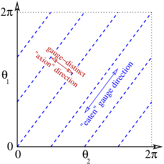
Figure 4: Space of $\varphi_{1},\varphi_{2}$ phases $(\theta_{1},\theta_{2})$ for the case $(q_{1},q_{2})=(4,3)$. The dashed (blue) line indicates phase pairs which are equivalent under gauge transformations. An appropriate vector potential can cancel any gradient energy in the direction of the dashed lines.

 

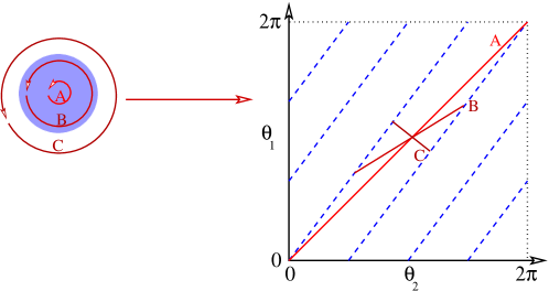
Figure 5: Left: cross-section of a string, showing the magnetic field strength “bundle” and three possible loops one can take around the center of the string. Right: path through $(\theta_{1},\theta_{2})$ space taken along each loop. As more magnetic flux is enclosed, the component of $(\Delta\theta_{1},\Delta\theta_{2})$ along the gauge-direction is canceled, but the component in the “global” direction is not.

For a more intuitive explanation, consider Figure 4. It shows the set of possible phases $(\theta_{1},\theta_{2})$ for the two scalar fields, in the case $(q_{1},q_{2})=(4,3)$. The figure includes a dotted line to indicate which phase choices are gauge-equivalent. Moving along the dotted line corresponds to changing the gauge, or moving through space along a gauge field; a vector potential of the right size can cancel a gradient energy along this field direction. The orthogonal direction, which is unaffected by a gauge field, is the global (axion) field direction. A change in this direction from one blue dotted line to the next represents a full $2\pi$ rotation in the (axial) Goldstone direction, which explains the value of $f_{a}$ found in Eq. (38). Figure 5 then shows how each field varies around a string. As we consider loops farther and farther from the string’s center, more and more flux is enclosed, so more and more of the gradients along the blue-dotted direction are canceled by the $A_{\phi}$ field. For the innermost loop there is no enclosed flux, and the gradient energy is given by the distance between the point $(\theta_{1},\theta_{2})=(0,0)$ to the point $(2\pi,2\pi)$. For a loop enclosing the entire flux, all gradient energy arising from the gauge-direction is canceled, almost but not fully removing the gradient energy. Only the gradient energy arising from the shortest path from one blue-dotted line to the next cannot be compensated. This represents the residual global charge of the string. This path length is $2\pi f_{a}$.

Now let us estimate the effective value of $\bar{\kappa}$, the added contribution to the string tension in units of the long-distance Goldstone-mode contribution. The energy of the string’s core is the energy of an abelian Higgs string with $m_{h}=m_{e}$ and with $f^{2}=v_{1}^{2}+v_{2}^{2}$, which is

$$T_{\mathrm{str,abelian}}\simeq\pi(v_{1}^{2}+v_{2}^{2})\,.$$ (39)

The value of $\bar{\kappa}$ is therefore

$$\bar{\kappa}=\frac{T_{\mathrm{str}}}{\pi f_{a}^{2}}\simeq\frac{v_{1}^{2}+v_{2}^{2}}{\frac{v_{1}^{2}v_{2}^{2}}{q_{1}^{2}v_{1}^{2}+q_{2}^{2}v_{2}^{2}}}=\frac{(v_{1}^{2}+v_{2}^{2})(q_{1}^{2}v_{1}^{2}+q_{2}^{2}v_{2}^{2})}{v_{1}^{2}v_{2}^{2}}\quad\longrightarrow_{v_{1}=v_{2}}\quad 2(q_{1}^{2}+q_{2}^{2})\,.$$ (40)

Detailed calculations show that this is indeed the added tension. The full value of $\kappa$ is $\kappa=\bar{\kappa}+\ln(m/H)$ where $m,H$ are the values actually used in the numerical simulation; typically $m/H\sim 1000$. So choosing $q_{1}=4$ and $v_{1}=v_{2}$ gives $\bar{\kappa}=50$ and $\kappa=57$, in the middle of the physically interesting range.

 

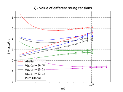
Figure 6: Network density for different string tensions. The falling curves represent the overdense networks, while the rising curves represent the underdense networks.

Figure 6 shows how the density of the string network depends on the string tension. The network density is expressed in terms of the dimensionless scaling variable $\xi$,

$$L_{\mathrm{sep}}^{-2}\equiv V^{-1}\int_{\mathrm{all\;string}}\gamma dl\,,\qquad\xi\equiv\frac{t^{2}}{4L^{2}}\,.$$ (41)

We see that it increases by over a factor of 3 as one goes from scalar-only ($\kappa\simeq 7$) to high-tension ($\kappa\simeq 57$) simulations. It is not clear that our lattices are large enough to see the onset of scaling behavior for the highest-tension networks we studied. We certainly don’t see scaling behavior for the abelian Higgs simulations, but this is another story.

5.4 Numerical implementation

I will not insult this audience by explaining how to implement a bosonic U(1) theory on the lattice. I use the noncompact formulation of U(1) and a next-nearest neighbor $(a^{2})$ improved action. There are no issues of renormalization of parameters because we are studying classical field theory. A subtlety in implementing electric fields with improvement is handled as in Moore:1996wn . We pause only to mention one subtlety in how we implement $\chi(1-\cos\theta_{\mathrm{a}})$. The function $\cos\theta_{\mathrm{a}}$, with $\theta_{\mathrm{a}}=q_{2}\theta_{1}-q_{1}\theta_{2}$, is highly singular near the string core. Such singular behavior creates problems under space discretization, so we have to “round off” the behavior inside the string core, with the substitution

$$\chi(t)\Big{(}1-\cos\theta_{\mathrm{a}}\Big{)} \Rightarrow\chi(t)F(2\varphi_{1}^{*}\varphi_{1})F(2\varphi_{2}^{*}\varphi_{2})\left(1-\cos\Big{(}q_{2}\,\mathrm{Arg}\,\varphi_{1}-q_{1}\,\mathrm{Arg}\,\varphi_{2}\Big{)}\right)\,,$$ (42)

$$F(r) \equiv\left\{\begin{array}[]{ll}\frac{25}{16}r\left(\frac{8}{5}-r\right)\,,&r<\frac{4}{5}\,,\\ 1\,,&r>\frac{4}{5}\,.\end{array}\right.$$ (45)

The smoothing function $F(r)$ is chosen such that $F(1)=1$, $F^{\prime}(1)=0$, $F(0)=0$, and $F^{\prime}(r)$ is continuous. This modification only affects the dynamics inside string cores, but the $\chi(t)(1-\cos\theta_{\mathrm{a}})$ term is much smaller than the other potential terms there. Indeed, this term is everywhere small and it is only important because it operates over much of the lattice volume, while the radial potential has an effect only in the tiny fraction of the lattice corresponding to string cores.

6 Results

We studied this model axion4 on $2048^{3}$ lattices using a single compute node containing two Xeon Phi (KNL) processors. After systematic studies of lattice spacing and continuum limits, we also studied how the network evolution and the axion production depend on the string tension.

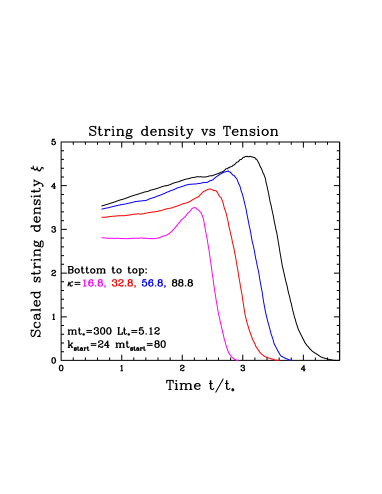
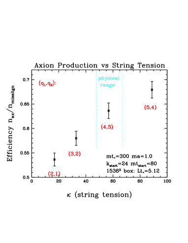
Figure 7: Left: string density as a function of time for different $\kappa$ values. The higher the string tension, the longer the strings persist. Right: axion production efficiency as a function of $\kappa$.

The most notable result is that the axion production is actually smaller for the case with strings than the angle-average of the “misalignment” mechanism of Eq. (14). This contradicts the “conventional wisdom” Hiramatsu:2012gg that axion production should be the sum of a misalignment contribution, a string contribution, and a wall contribution. We claim that this view double counts; the energy in domain walls is the energy of field misalignment, from values $\theta_{\mathrm{a}}\sim\pi$. This energy represents most of the potential axion production from misalignment. But the energy in the wall network is mostly absorbed by the strings when the walls pull on the strings, giving their energy to string velocity. Then the strings chop up into loops, which appear to produce axions quite inefficiently.

Combining our numbers with expressions for the energy budget $g_{*}$ and topological susceptibility from Borsanyi:2016ksw , and the observed dark matter density, we find $m_{a}=26.2\pm 3.4\,\mu\mathrm{eV}$.

7 Topology: temperature range

We have emphasized that an input value for $\chi(T)$ from the lattice is essential to deriving these results. But we don’t need $\chi(T)$ at all temperatures; some are more important than others. We will extend the results of axion4 by investigating over what temperature range the topological susceptibility is really needed.

At sufficiently high temperature $\chi(T)$ is small. Therefore $\chi(T)(1-\cos\theta_{\mathrm{a}})$ plays little role in the field dynamics. Its importance is controlled by the combination $m_{a}t$ which rises with time as approximately $t^{5.8}$. Therefore at high temperature, large errors in $\chi(T)$, or no value at all, is not a problem. To study this, we replace $\chi(T)$ with the following “chopped” form:

$$\chi(T)\to\left\{\begin{array}[]{ll}\chi(T)&T<T_{\mathrm{chop}}\\ \chi(T_{\mathrm{chop}})&T>T_{\mathrm{chop}}\,.\\ \end{array}\right.$$ (46)

Technically it is $t^{2}\chi(T)$ we chop in this way, because of the $t^{2}$ factor in, eg, Eq. (14). We then study the axion production as a function of the temperature $T_{\mathrm{chop}}$. When $n_{\mathrm{ax}}$ ceases to depend on $T_{\mathrm{chop}}$, we know that $\chi(T_{\mathrm{chop}})$ is not relevant. But so long as the result with $T_{\mathrm{chop}}$ is different than the unchopped limit, we need $\chi(T)$ at that temperature.

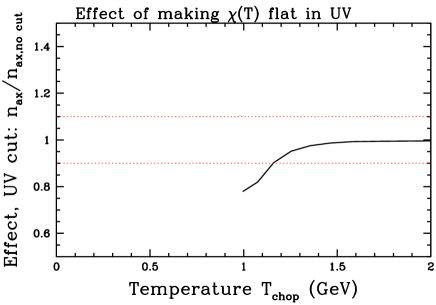
Figure 8: Effect of replacing $\chi(T)$ with a result which is flat in the UV, to diagnose at what scale we need to compute $\chi(T)$.

We see from Fig.8 that above about 1150 MeV, it makes little difference if we change $\chi(T)$. But below this value, we are quite sensitive. So it is necessary to determine $\chi(T)$ all the way up to 1150 MeV.

On the IR side, perhaps surprisingly, there is also a range of temperatures where the susceptibility is not important. That is because the strings and walls are gone and the $\theta_{\mathrm{a}}$ value is small and oscillating rapidly, with $m_{a}\gg H$. Then the axion number is an approximate adiabatic invariant, which reacts smoothly to Hubble expansion and mass shifts and does not feel the anharmonicity of the potential, $1-\cos\theta_{\mathrm{a}}\simeq\theta_{\mathrm{a}}^{2}/2$. All that matters is the final value of $\chi(T\to 0)$, which is well known. To find out where this temperature range starts, we make a similar modification:

$$\chi(T)\to\left\{\begin{array}[]{ll}\chi(T)&T>T_{\mathrm{chop}}\\ \chi(T_{\mathrm{chop}})&T<T_{\mathrm{chop}}\,.\\ \end{array}\right.$$ (47)

That is, we freeze $\chi(T)$ (really, $t^{2}\chi(T)$) from rising after some point, and see if that changes the axion number produced.

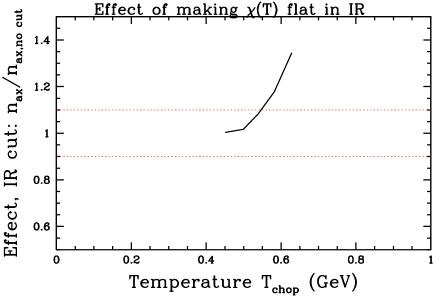
Figure 9: Effect of replacing $\chi(T)$ with a result which is flat in the IR, to diagnose at what temperature we first need to know $\chi(T)$.

The results are shown in Fig. 9. They indicate that the susceptibility is irrelevant below about 550 MeV; the behavior above that temperature is important. Therefore the axion dynamics is sensitive to $\chi(T)$ in the range 550 to 1150 MeV; outside of that range it is not.

8 Conclusions

The axion is a well motivated hypothetical particle, because it might explain two mysteries – the P and T symmetry of QCD, and the nature of the Dark Matter – with a single mechanism and particle. The physics of the axion in cosmology is rich, governed by a network of string defects which are swept together when domain walls form. Its explication requires two new pieces of physics. We need to understand this network evolution and axion production better. And we need to know the QCD topological susceptibility as a function of temperature, $\chi(T)$, because it sets the tension of the domain walls and controls the physics which destroys the string network. I have presented the latest details on the network evolution, introducing a new technique which allows simulation of high-tension strings without excessive numerical resources. The results indicate rather inefficient axion production and therefore a rather light axion compared to previous studies, with $m_{a}=26.2\pm 3.4\,\mu\mathrm{eV}$.

It remains to form a consensus in the lattice community that the topological susceptibility is well measured. My work indicates that the susceptibility is needed in a temperature range from 550 to 1150 MeV. Below this range the evolution is adiabatic. Above this range the susceptibility does not yet play a role in axion dynamics. Clearly it is challenging to determine the susceptibility at such high temperatures. But I am confident this is a challenge which the lattice community will accept with gusto.

References

- (1) R. Peccei, H.R. Quinn, Phys.Rev.Lett. 38, 1440 (1977)
- (2) R. Peccei, H.R. Quinn, Phys.Rev. D16, 1791 (1977)
- (3) S. Weinberg, Phys.Rev.Lett. 40, 223 (1978)
- (4) F. Wilczek, Phys.Rev.Lett. 40, 279 (1978)
- (5) G. ’t Hooft, Phys.Rev. D14, 3432 (1976)
- (6) R. Jackiw, C. Rebbi, Phys. Rev. Lett. 37, 172 (1976)
- (7) C.G. Callan, Jr., R.F. Dashen, D.J. Gross, Phys. Rev. D20, 3279 (1979)
- (8) J. Preskill, M.B. Wise, F. Wilczek, Phys. Lett. B120, 127 (1983)
- (9) L.F. Abbott, P. Sikivie, Phys. Lett. B120, 133 (1983)
- (10) M. Dine, W. Fischler, Phys. Lett. B120, 137 (1983)
- (11) C.A. Baker et al., Phys. Rev. Lett. 97, 131801 (2006), hep-ex/0602020
- (12) F.K. Guo, R. Horsley, U.G. Meissner, Y. Nakamura, H. Perlt, P.E.L. Rakow, G. Schierholz, A. Schiller, J.M. Zanotti, Phys. Rev. Lett. 115, 062001 (2015), 1502.02295
- (13) M. Abramczyk, S. Aoki, T. Blum, T. Izubuchi, H. Ohki, S. Syritsyn, Phys. Rev. D96, 014501 (2017), 1701.07792
- (14) K.F. Liu, J. Liang, Y.B. Yang (2017), 1705.06358
- (15) K. Fujikawa, Phys. Rev. Lett. 42, 1195 (1979)
- (16) K. Fujikawa, Phys. Rev. D21, 2848 (1980), [Erratum: Phys. Rev.D22,1499(1980)]
- (17) J.E. Kim, Phys. Rev. Lett. 43, 103 (1979)
- (18) M.A. Shifman, A.I. Vainshtein, V.I. Zakharov, Nucl. Phys. B166, 493 (1980)
- (19) G. Grilli di Cortona, E. Hardy, J.P. Vega, G. Villadoro, JHEP 01, 034 (2016), 1511.02867
- (20) D.J. Gross, R.D. Pisarski, L.G. Yaffe, Rev. Mod. Phys. 53, 43 (1981)
- (21) E. Berkowitz, M.I. Buchoff, E. Rinaldi, Phys. Rev. D92, 034507 (2015), 1505.07455
- (22) S. Borsanyi, M. Dierigl, Z. Fodor, S.D. Katz, S.W. Mages, D. Nogradi, J. Redondo, A. Ringwald, K.K. Szabo, Phys. Lett. B752, 175 (2016), 1508.06917
- (23) P. Petreczky, H.P. Schadler, S. Sharma, Phys. Lett. B762, 498 (2016), 1606.03145
- (24) Y. Taniguchi, K. Kanaya, H. Suzuki, T. Umeda, Phys. Rev. D95, 054502 (2017), 1611.02411
- (25) F. Burger, E.M. Ilgenfritz, M.P. Lombardo, M. MÃller-Preussker, A. Trunin, Topology (and axion’s properties) from lattice QCD with a dynamical charm, in 26th International Conference on Ultrarelativistic Nucleus-Nucleus Collisions (Quark Matter 2017) Chicago,Illinois, USA, February 6-11, 2017 (2017), 1705.01847, https://inspirehep.net/record/1598136/files/arXiv:1705.01847.pdf
- (26) J. Frison, R. Kitano, H. Matsufuru, S. Mori, N. Yamada, JHEP 09, 021 (2016), 1606.07175
- (27) S. Borsanyi et al., Nature 539, 69 (2016), 1606.07494
- (28) C. Bonati, M. D’Elia, M. Mariti, G. Martinelli, M. Mesiti, F. Negro, F. Sanfilippo, G. Villadoro, JHEP 03, 155 (2016), 1512.06746
- (29) C. Bonati, M. D’Elia, M. Mariti, G. Martinelli, M. Mesiti, F. Negro, F. Sanfilippo, G. Villadoro, EPJ Web Conf. 137, 08004 (2017), 1612.06269
- (30) L. Visinelli, P. Gondolo, Phys. Rev. Lett. 113, 011802 (2014), 1403.4594
- (31) P.A.R. Ade et al. (Planck), Astron. Astrophys. 594, A13 (2016), 1502.01589
- (32) T.W.B. Kibble, J. Phys. A9, 1387 (1976)
- (33) A. Albrecht, N. Turok, Phys. Rev. Lett. 54, 1868 (1985)
- (34) R.L. Davis, Phys. Lett. B180, 225 (1986)
- (35) A. Dabholkar, J.M. Quashnock, Nucl. Phys. B333, 815 (1990)
- (36) L. Fleury, G.D. Moore, Journal of Cosmology and Astroparticle Physics 2016, 004 (2016), 1509.00026
- (37) V.B. Klaer, G.D. Moore (2017), 1707.05566
- (38) T. Goto, Prog. Theor. Phys. 46, 1560 (1971)
- (39) P. Goddard, J. Goldstone, C. Rebbi, C.B. Thorn, Nucl. Phys. B56, 109 (1973)
- (40) Y. Nambu, Phys. Rev. D10, 4262 (1974)
- (41) M. Kalb, P. Ramond, Phys. Rev. D9, 2273 (1974)
- (42) A. Vilenkin, T. Vachaspati, Phys. Rev. D35, 1138 (1987)
- (43) C.T. Hill, A.L. Kagan, L.M. Widrow, Phys. Rev. D38, 1100 (1988)
- (44) G.D. Moore, Nucl. Phys. B480, 689 (1996), hep-lat/9605001
- (45) V.B. Klaer, G.D. Moore (2017), 1708.07521
- (46) T. Hiramatsu, M. Kawasaki, K. Saikawa, T. Sekiguchi, Phys.Rev. D85, 105020 (2012), 1202.5851