Fighting topological freezing in the two-dimensional CP^N-1 model

Abstract

We perform Monte Carlo simulations of the CP^N-1 model on the square lattice for $N=10$, $21$, and $41$. Our focus is on the severe slowing down related to instantons. To fight this problem we employ open boundary conditions as proposed by Lüscher and Schaefer for lattice QCD. Furthermore we test the efficiency of parallel tempering of a line defect. Our results for open boundary conditions are consistent with the expectation that topological freezing is avoided, while autocorrelation times are still large. The results obtained with parallel tempering are encouraging.

1 Introduction

The CP^N-1 model shares fundamental properties such as asymptotic freedom and confinement with QCD. Therefore it serves as a toy model of QCD. It has been shown DAdda:1978vbw ; Witten79 that the model has a non-trivial vacuum structure with stable instanton solutions. It turned out that these topological objects pose a particular problem in the simulation of the lattice CP^N-1 model, similar to lattice QCD.

On the torus, in the continuum limit, the configuration space is decomposed into sectors that are characterized by their topological charge. At finite lattice spacing, the free energy barriers between such sectors increase as the lattice spacing decreases. For Markov chain Monte Carlo algorithms that walk in a quasi continuous fashion through configuration space this means that they become essentially non-ergodic and slowing down becomes dramatic. Numerical results are compatible with an increase of autocorrelation times that is exponential in the inverse lattice spacing. In the case of the CP^N-1 model this is numerically verified, for example, in refs. Campostrini ; Vicari04 ; Flynnetal15 . Modelling the autocorrelation times with a more conventional power law Ansatz, large powers are needed to fit the data. From a practical point of view, the consequence is that it becomes virtually impossible to access lattice spacings below a certain threshold. The numerical studies show that in the case of the CP^N-1 model the problem becomes worse with increasing $N$. Since it is much less expensive to simulate the two-dimensional model than lattice QCD, it is a good test bed for new ideas and algorithms that could overcome the severe slowing down of the topological modes. For example simulated tempering MaPa92 has been studied in ref. Vicari92 with moderate success. More recently, “trivializing maps in the Hybrid Monte Carlo algorithm” Engel:2011re or the “Metadynamics” method Metadynamics have been tested.

A very principle solution of the problem had been suggested in ref. Luscher:2011kk . By abandoning periodic boundary conditions in one of the directions in favour of open ones, barriers between the topological sectors are abolished. The proposal has been further tested Luscher:2012av ; McGlMa14 and adopted in large scale simulations of lattice QCD with dynamical fermions Bruno:2014ova ; CLS . Here we shall probe in detail how open boundary conditions effect the slowing down in the case of the CP^N-1 model. Since the CP^N-1 model is much cheaper to simulate than lattice QCD, a larger range of lattice spacings can be studied and autocorrelation functions can be computed more accurately.

Furthermore, we shall explore parallel tempering SW86 ; raex ; Hukushima:1996xx ; Earl:2005xx as a solution to our problem. Parallel tempering is a well established approach in statistical physics to overcome effective non-ergodicity due to a ragged free energy landscape. The idea of parallel tempering and similar methods is to enlarge the configuration space such that the hills can be easily by-passed. A prototype problem is the study of spin-glasses, where parallel tempering is mandatory. For recent work see for example ref. Janus2013 . Typically a global parameter such as the temperature or an external field is used as parameter of the tempering. Here instead, we shall discuss a line defect.

Finally we like to mention that for the CP^N-1 model dual formulations can be found. These can be simulated by using the worm algorithm Prokofev:2001ddj ; Ulli . In these dual formulations there are no topological sectors and hence severe slowing down does not occur in the simulation.

2 The model

We consider a square lattice with sites $x=(x_{0},x_{1})$, where $x_{i}\in\{0,1,2,...,L_{i}-1\}$. The lattice spacing is set to $a=1$. This means that we trade a decreasing lattice spacing for an increasing correlation length. The action is

$$S=-\beta N\sum_{x,\mu}\left(\bar{z}_{x+\hat{\mu}}z_{x}\lambda_{x,\mu}+z_{x+\hat{\mu}}\bar{z}_{x}\bar{\lambda}_{x,\mu}-2\right)\;,$$ (1)

where $z_{x}$ is a complex $N$-component vector with $z_{x}\bar{z}_{x}=1$ and $\lambda_{x,\mu}$ is a complex number with $\lambda_{x,\mu}\bar{\lambda}_{x,\mu}=1$. The gauge fields live on the links, which are denoted by $x,\mu$, where $\mu\in\{0,1\}$ gives the direction and $\hat{\mu}$ is a unit vector in $\mu$-direction. In $1$-direction we always consider periodic boundary conditions. In $0$-direction either open or periodic boundary conditions are considered. We implement open boundary conditions in a crude way, simply setting $\beta=0$ for the links that connect $x_{0}=L_{0}-1$ and $x_{0}=0$.

2.1 The observables

We measure the energy, the magnetic susceptibility, the second moment and the exponential correlation length. For the definition of these quantities see for example ref. Campostrini or section II A of ref. MyCPN . Our main focus is on the topology of the field. Motivated by eq. (33) of ref. Campostrini we define the plaquette angle

$$\theta_{plaq,x}=\theta_{x,\mu}+\theta_{x+\hat{\mu},\nu}-\theta_{x+\hat{\nu},\mu}-\theta_{x,\nu}-2n\pi\;\;\;,\;\;\;\;\;\;\mu\neq\nu\;,$$ (2)

where $\theta_{x,\mu}=\mbox{arg}\{\bar{z}_{x}z_{x+\hat{\mu}}\}$ and the integer $n$ is chosen such that $-\pi<\theta_{plaq,x}\leq\pi$. We define the topological charge density $q_{x}=\frac{1}{2\pi}\theta_{plaq,x}$. The topological charge on the lattice with periodic boundary conditions is defined by

$$Q=\sum_{x}q_{x}=\frac{1}{2\pi}\sum_{x}\theta_{plaq,x}\;.$$ (3)

The topological susceptibility is then given by

$$\chi_{t}=\frac{1}{V}\langle Q^{2}\rangle=\frac{1}{L_{0}L_{1}}\left\langle\sum_{xy}q_{x}q_{y}\right\rangle=\frac{1}{L_{0}L_{1}}\left\langle\sum_{x_{0}x_{1}}q_{x_{0},x_{1}}\sum_{y_{0}y_{1}}q_{y_{0}y_{1}}\right\rangle=\frac{1}{L_{0}}\left\langle\sum_{x_{0}}\tilde{q}_{x_{0}}\sum_{y_{0}}\tilde{q}_{y_{0}}\right\rangle\;,$$ (4)

where we define $\tilde{q}_{x_{0}}=\frac{1}{\sqrt{L_{1}}}\sum_{x_{1}}q_{x_{0},x_{1}}$. Note that the definition of the topological charge given in ref. Berg:1981er and (3) are not equivalent at finite lattice spacing. We checked numerically that the difference between the two definitions decreases quickly with increasing $\beta$. Also cooling of the configurations strongly reduces the difference.

On the lattice with periodic boundary conditions, $Q$ can take only integer values. Naively, $\theta_{plaq,x}$ adds up to zero, since each link angle appears with both signs. A nontrivial result is due to the fact that $\theta_{plaq,x}$ is thrown back to the interval $[-\pi,\pi)$.

In the case of open boundary conditions, the definitions of susceptibilities have to be adapted. In order to avoid large finite size effects, the sites with a distance less than $l_{0}$ from the open boundary are not taken into account, when computing the observables. Motivated by the rightmost part of eq. (4) we arrive at

$$\chi_{t,open}=\frac{1}{L_{0}-2l_{0}}\sum_{x_{0}=l_{0}}^{L_{0}-l_{0}-1}\langle\tilde{q}_{x_{0}}^{2}\rangle\;+2\sum_{w=1}^{l_{max}}\frac{1}{L_{0}-2l_{0}-w}\sum_{x_{0}=l_{0}}^{L_{0}-l_{0}-w-1}\langle\tilde{q}_{x_{0}}\tilde{q}_{x_{0}+w}\rangle\;\;.$$ (5)

3 Basic algorithms

As basic algorithm we use a hybrid of the Metropolis, the heat bath and the microcanonical overrelaxation algorithm. To a large extend, we follow section III of ref. Campostrini . Let us first discuss the updates of the site variables and then the updates of the gauge fields. In an elementary step of the algorithm we update the variable at a single site $x$, while keeping the gauge fields and the variables at all other sites fixed. The part of the action that depends on this site variable can be written as as

$$\tilde{S}(z_{x})=-\mbox{Re}\;z_{x}\bar{F}_{x}\;,\;\;\mbox{where}\;\;F_{x}=2N\beta\;\sum_{\mu}\left[\bar{\lambda}_{x,\mu}z_{x+\hat{\mu}}+\lambda_{x-\hat{\mu},\mu}z_{x-\hat{\mu}}\right]\;.$$ (6)

Note that the problem at this point is identical to the update of an O$(2N)$ invariant vector model with site variables of unit length. Instead of $\bar{F}_{x}$ we would have to deal with the sum of the variables on the nearest neighbour sites. The microcanonical update keeps $\tilde{S}(z_{x})$ fixed, while the new value of $z_{x}$ has maximal distance from the old one. It is given by eq. (43a) of ref. Campostrini :

$$z_{x}^{\prime}=2\frac{\mbox{Re}\;z_{x}\bar{F}_{x}}{|F_{x}|^{2}}F_{x}-z_{x}\;.$$ (7)

In addition to these updates, we have to perform updates that change the value of the action. To this end we implemented a heat bath algorithm that is applied to the subset of three of the $2N$ components of $z_{x}$, where we count both the real and the imaginary parts. The heat bath update is identical to the one used in the simulation of the O(3)-Heisenberg model on the lattice or for the update of SU$(2)$ subgroups in the simulation of pure SU$(N)$ lattice gauge models CM82 ; Cr80 . We run through all $N$ complex components of $z_{x}$ taking the real and the imaginary part of the component as first two components for the heat bath. The third component is randomly chosen among the real or imaginary parts of the remaining $N-1$ components of $z_{x}$. Note that the CPU-time required by the microcanonical overrelaxation update is about one order of magnitude less than that for the heat bath update.

For fixed variables $z$ the gauge fields can be updated independently of each other. The action reads

$$\tilde{S}_{g}(\lambda_{x,\mu})=-\mbox{Re}\lambda_{x,\mu}\bar{f}_{x,\mu}\;,\;\;\mbox{where}\;\;f_{x,\mu}=2N\beta\;z_{x+\hat{\mu}}\bar{z}_{x}\;.$$ (8)

Here we perform a four hit Metropolis update, where the stepsize was chosen such that the acceptance rate is roughly $50\%$, and a microcanonical update, see eq. (43b) of Campostrini .

3.1 Autocorrelation times

The performance of a Markov chain Monte Carlo algorithm is characterized by the autocorrelation time. There are different definitions of the autocorrelation time. These are based on the autocorrelation function. The autocorrelation function of an estimator $A$ is given by

$$\rho_{A}(t)=\frac{\langle A_{i}A_{i+t}\rangle-\langle A\rangle^{2}}{\langle A^{2}\rangle-\langle A\rangle^{2}}\;.$$ (9)

The modulus of the autocorrelation function is bounded from above by an exponentially decaying function. In practice one often finds that the autocorrelation function at large $t$ is given by $\rho_{A}(t)\simeq c_{A}\exp(-t/\tau_{exp,A})$. The integrated autocorrelation time of the estimator $A$ is given by

$$\tau_{int,A}=0.5+\sum_{t=1}^{\infty}\rho_{A}(t)\;.$$ (10)

The summation in eq. (10) has to be truncated at some finite $t_{max}$. Since $\rho_{A}(t)$ is falling off exponentially at large distances, the relative statistical becomes large at large distances. Therefore it is mandatory to truncate the summation at some point that is typically much smaller than the total length of the simulation. In the literature one can find various recommendations how this upper bound should be chosen. Fore example, Wolff Wolff:2003sm proposes to balance the statistical error with the systematic one that is due to the truncation of the sum.

4 Simulations with open boundary conditions

In order to keep the fraction of discarded sites small, it seems useful to chose $L_{0}\gg L_{1}$. On the other hand, since the time needed for topological objects to diffuse to the centre of the lattice or back to the boundary increases with increasing $L_{0}$, too large values of $L_{0}$ are not advisable. After performing preliminary simulations we decided to take $L_{0}=4L_{1}$ throughout. Furthermore we take $l_{0}\approx 10\xi_{2nd}$ and $l_{max}=l_{0}$. For $N=10$, using standard simulations and periodic boundary conditions, $\xi_{2nd}\approx 23$ can be reached Flynnetal15 . Hence it is hard to demonstrate a clear advantage for open boundary conditions. Instead for $N=21$ it is virtually impossible to go beyond $\xi_{2nd}\approx 6$ by using periodic boundary conditions and standard simulations. Therefore in the following we focus on our simulations for $N=21$. We find that for $L_{1}\gtrapprox 16\xi_{2nd}$ finite $L_{1}$ effects can be ignored at the level of our statistical accuracy. We performed simulations for a large number of $\beta$-values, ranging from $\beta=0.625$ up to $0.95$. For each value of $\beta$, we performed $2\times 10^{6}$ update cycles. For the larger values of $\beta$, we discarded $50000$ update cycles at the beginning of the simulation. One update cycle consists of one sweep over all sites of the lattice using the heat bath algorithm, the 4 hit Metropolis update of the gauge fields, and finally $n_{ov}$ sweeps using the overrelaxation algorithm for both the site variables and the gauge fields. We perform a measurement of the observables for each cycle. Autocorrelation times are quoted in units of these update cycles. The number of overrelaxation updates $n_{ov}$ is chosen to be proportional to the correlation length. It increases from $n_{ov}=3$ for $\beta=0.625$ up to $n_{ov}=28$ for $\beta=0.95$. The second moment correlation length increases from $\xi_{2nd}=2.2968(5)$ at $\beta=0.625$ up to $18.2419(43)$ at $\beta=0.95$.

Figure 1: We plot the integrated autocorrelation time $\tau_{int}$ of the topological susceptibility for both periodic and open boundary conditions as a function of the second moment correlation length $\xi_{2nd}$ for $N=21$. Here $\tau_{int}$ is given in units of update cycles. For large $\xi_{2nd}$ the effort for one update cycle is proportional to the number of overrelaxation sweeps $n_{ov}$. Hence, the plateau of $\tau_{int}$ corresponds to a dynamical critical exponent $z\approx 1$, taking single sweeps as unit of time.

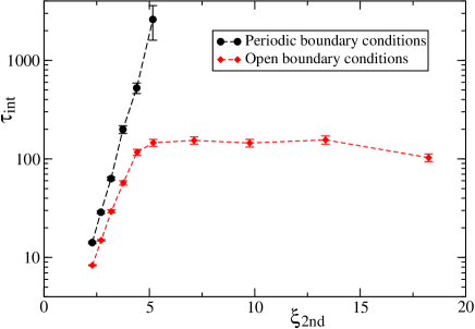
Let us discuss the autocorrelation times of the topological susceptibility (4,5). For periodic boundary conditions, $\tau_{int}$ increases very rapid, compatible with exponential in the correlation length. Instead, for open boundary conditions, we first see an increase that is similar to that for periodic boundary conditions. The difference here can be attributed to the different definitions of the topological susceptibility (4,5). Then, for $\xi_{2nd}\gtrapprox 5$ the autocorrelation time levels off for open boundary conditions.

The behaviour in the case of open boundary conditions can be explained along the lines of ref. McGlMa14 . For $\xi_{2nd}\lessapprox 5$ changes of the topological charge are dominantly due to the creation and destruction of instantons in the bulk. Then for $\xi_{2nd}\gtrapprox 5$ the diffusion from and to the boundaries completely dominates. This diffusion is not effected by the severe slowing down. Our numerical results for $N=41$ confirm the conclusions drawn here for $N=21$.

5 Parallel tempering in a line defect

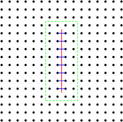
In a parallel tempering simulation one introduces a sequence of $N_{t}$ systems that differ in one parameter of the action. For each system there is a configuration $\{z,\lambda\}_{t}$. The tempering parameter might have a physical meaning. In statistical physics simulations this parameter is mostly the temperature. However it could also be a parameter that is introduced only for the sake of the simulation, as it is the case here. At one end of the sequence there is the system that we want to study. In our case this is a lattice with $L_{0}=L_{1}$, periodic boundary conditions in both directions, and the coupling constant is the same for all links. For the system at the other end, it should be easy to sample the whole configuration space. Motivated by the success of the simulations with open boundary conditions, we use a system with a line defect to this end. Such a line defect is sketched in fig. 2. For $l_{d}=L_{1}$ we recover open boundary conditions.

Figure 2: Sketch of a line defect. The red line indicates a line defect of length $l_{d}$. The coupling on the blue links is reduced or, in the extreme case, completely switched off. In our simulations we take for simplicity a linear interpolation: The couplings on the blue links are multiplied by $c_{r}(t)=1-t/(N_{t}-1)$. The homogeneous system corresponds to $t=0$, while for $t=N_{t}-1$ the coupling along the defect line is completely eliminated. The green lines confine the area of a rectangle centred around the defect line. The size of the rectangle is $2l_{i}\times(l_{d}+2l_{i})$, where $i$ gives the level. In our simulations $l_{i+1}=l_{i}/2$ for $i>1$. For each update cycle at level $i$ we perform $n_{i+1}$ update cycles at level $i+1$. At level $i=0$ we sweep over the whole lattice. $l_{1}=2^{m}$, where $m$ is an integer and $l_{1}\approx\xi$. Furthermore $l_{i_{max}}=1$.

In addition to updates of the individual systems there are exchanges of configurations between the systems. A swap of configurations $\{z,\lambda\}_{t_{1}}^{\prime}=\{z,\lambda\}_{t_{2}}$, $\{z,\lambda\}_{t_{2}}^{\prime}=\{z,\lambda\}_{t_{1}}$ between $t_{1}$ and $t_{2}$ is accepted with the probability

$$A_{swap}=\mbox{min}\left[1,\exp\left(-S_{t_{2}}(\{z,\lambda\}_{t_{1}})-S_{t_{1}}(\{z,\lambda\}_{t_{2}})+S_{t_{1}}(\{z,\lambda\}_{t_{1}})+S_{t_{2}}(\{z,\lambda\}_{t_{2}})\right)\right]\;.$$ (11)

In our simulations we run from $t_{1}=0$ up to $t_{1}=N_{t}-2$ in steps of one, proposing to swap the configurations at $t_{1}$ and $t_{2}=t_{1}+1$. The number of replica $N_{t}$ is chosen such that the acceptance rate for the swap of configurations is larger than $30\%$ for all $t_{1}$. Note that $S_{t_{2}}$ and $S_{t_{1}}$ differ only on the defect line. Typically the swap of configurations is alternating with standard updates of the individual configurations. Typically, when the tempering parameter is homogeneous in space, a sweep over the whole lattice is performed. In contrast, here we temper in a defect that takes only a small fraction of the lattice. Therefore it is advisable to update only some part of the lattice that is centred around the defect. To this end, we introduce a sequence of rectangles of decreasing size, each associated with a level of our update scheme. For details see Fig. 2. In one update cycle, at a given level, we sweep over the rectangle, updating all $N_{t}$ configurations: Once using the heat bath algorithm for the site variables and the 4 hit Metropolis update for the gauge fields. Then follow $n_{ov,i}$ overrelaxation sweeps of the site variables and the gauge fields. For small $i$, $n_{ov,i}$ is the same as for our simulations with open boundary conditions. For larger $i$, smaller values are taken. The update cycle at a given level is completed by a swap of configurations (11). We chose $n_{i}$ such that for each level of the update scheme, roughly the same amount of CPU time is spent. The larger $l_{d}$, the more topological objects can be generated or destroyed. On the other hand, for increasing $l_{d}$, $N_{t}$ has to be enlarged to keep the acceptance rate above $30\%$. Our numerical study shows that $l_{d}\approx\xi$ is the optimal choice. We perform a translation of the configuration for $t=0$ after each swap. This way changes in the topology are injected at any location on the lattice and diffusion is not needed.

We performed simulations for $N=10$, $21$, and $41$ and various values of $\beta$. Let us discuss the simulation for $N=21$ and $\beta=0.95$ in more detail. We used $l_{d}=16$ and $N_{t}=32$. The complete update cycle over all levels is characterized by $n_{1}=24$, $n_{2}=n_{3}=n_{4}=3$, and $n_{5}=n_{6}=2$. The number of overrelaxation updates per cycle is $28$, $14$, $7$, $7$, $3$, and $3$ at levels $1$, $2$, $3$, $4$, $5$, and $6$, respectively. We find that the acceptance rate is about $81.4\%$ for the pair $t=0$ and $1$. It drops to $39.4\%$ for the pair $t=26$ and $27$. Then it increases again to $47.3\%$ for the pair $t=30$ and $31$. The simulation, consisting of 50370 complete update cycles over all levels, took 25 days on a 4 core PC running with 8 threads. This is about the same CPU time that is used for the corresponding run with open boundary conditions. The error bar of the topological susceptibility is smaller by a factor of $2.3$ compared with the simulation with open boundary conditions.

6 Physics results and comparison with the large $N$-expansion

Following ref. CaRo91

$$\frac{\xi_{2nd}}{\xi_{exp}}=\sqrt{\frac{2}{3}}+O\left(N^{-2/3}\right)\;.$$ (12)

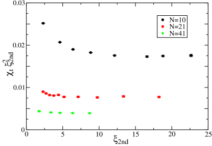
Our results obtained for $N=10$, $21$ and $41$, which are plotted in Fig. 3 a are still quite far from this asymptotic value. Therefore we abstain from estimating the coefficient of the $O(N^{-2/3})$ corrections.

The product $\chi_{t}\xi^{2}$ should have a finite continuum limit. For the exponential correlation length the $1/N$-expansion gives ML78

$$\chi_{t}\xi_{exp}^{2}=\frac{3}{4\pi N}+O\left(N^{-5/3}\right)\;\;.$$ (13)

For the second moment correlation length a faster convergence with increasing $N$ is obtained CaRo91

$$\chi_{t}\xi_{2nd}^{2}=\frac{1}{2\pi N}\left(1-\frac{0.38088...}{N}\right)+O\left(N^{-3}\right)\;.$$ (14)

(a) We plot the ratio $\xi_{exp}/\xi_{2nd}$ as a function of $\xi_{2nd}$.

(b) We plot $\xi_{2nd}^{2}\chi_{t}$ as a function of $\xi_{2nd}$.

Figure 3: Physics results for $N=10$, $21$ and $41$.

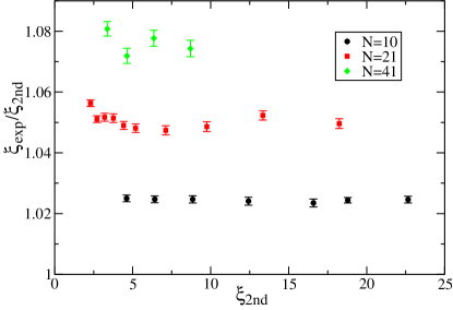
In Fig. 3 b we plot $\xi_{2nd}^{2}\chi_{t}$ as a function of $\xi_{2nd}$. Looking at the figure, the numerical data seem to converge nicely to the scaling limit. Corrections to scaling seem to be smaller for larger values of $N$. Taking simply the largest values of $\beta$ for each $N$ we get $\xi_{2nd}^{2}\chi_{t}=0.01737(8)$, $0.00767(5)$, and $0.00391(2)$ for $N=10$, $21$, and $41$, respectively. This can be compared with results quoted in the literature. For $N=10$ one finds for example $\xi_{2nd}^{2}\chi_{t}=0.01719(10)(3)$ and $0.0175(3)$ in refs. Flynnetal15 ; Vicari04 , respectively. For $N=21$ one finds $\xi_{2nd}^{2}\chi_{t}=0.0080(2)$ and $0.0076(3)$ in refs. Vicari04 ; Vicari92 , respectively. For $N=41$ we find in ref. Vicari92 the results $\xi_{2nd}^{2}\chi_{t}=0.0044(4)$ and $0.0036(4)$ for $\beta=0.57$ and $0.6$, respectively. Our estimates are essentially consistent with those presented in the literature. In particular for large values of $N$, we improved the accuracy of the estimates. To see the effect of leading corrections, it is useful to multiply $\xi_{2nd}^{2}\chi_{t}$ by $2\pi N$. Using our numbers, we get $1.091(5)$, $1.012(7)$, and $1.007(5)$ for $N=10$, $21$, and $41$, respectively. As already discussed in ref. Vicari04 it is a bit puzzling that the numbers suggest a $1/N$ correction with the opposite sign as that of eq. (14).

7 Summary and conclusions

We have shown that the severe slowing down in the simulation of the lattice CP^N-1 model can be avoided by using open boundary conditions in one of the directions. We studied parallel tempering in a line defect as an alternative. Our numerical results are encouraging. Focussing on the statistical error of the topological susceptibility, the simulation with open boundary conditions is outperformed by a factor of about 4. The crucial question is, of course, whether parallel tempering in a defect structure is helpful in simulations of lattice QCD. A more detail account of this study is given in MyCPN .

References

- (1) A. D’Adda, M. Lüscher, P. Di Vecchia, Nucl. Phys. B146, 63 (1978)
- (2) E. Witten, Nuovo Cim. A51, 325 (1979)
- (3) M. Campostrini, P. Rossi, E. Vicari, Phys. Rev. D46, 2647 (1992)
- (4) L. Del Debbio, G.M. Manca, E. Vicari, Phys. Lett. B594, 315 (2004), hep-lat/0403001
- (5) J. Flynn, A. Jüttner, A. Lawson, F. Sanfilippo (2015), 1504.06292
- (6) E. Marinari, G. Parisi, Europhys. Lett. 19, 451 (1992), hep-lat/9205018
- (7) E. Vicari, Phys. Lett. B309, 139 (1993), hep-lat/9209025
- (8) G.P. Engel, S. Schaefer, Comput. Phys. Commun. 182, 2107 (2011), 1102.1852
- (9) A. Laio, G. Martinelli, F. Sanfilippo, JHEP 07, 089 (2016), 1508.07270
- (10) M. Lüscher, S. Schaefer, JHEP 07, 036 (2011), 1105.4749
- (11) M. Lüscher, S. Schaefer, Comput. Phys. Commun. 184, 519 (2013), 1206.2809
- (12) G. McGlynn, R.D. Mawhinney, Phys. Rev. D90, 074502 (2014), 1406.4551
- (13) M. Bruno, S. Schaefer, R. Sommer (ALPHA), JHEP 08, 150 (2014), 1406.5363
- (14) M. Bruno et al., JHEP 02, 043 (2015), 1411.3982
- (15) Swendsen, Robert H. and Wang, Jian-Sheng, Phys.Rev.Lett. 57, 2607 (1986)
- (16) Geyer, C. J., Markov chain Monte Carlo maximum likelihood, in Computer Science and Statistics: Proc. of the 23rd Symposium on the Interface, edited by Keramidas, E. M. (Interface Foundation, Fairfax Station, 1991), p. 156
- (17) Hukushima, Koji and Nemoto, Koji, J.Phys.Soc.Jpn. 65, 1604 (1996), cond-mat/9512035
- (18) Earl, David J. and Deem, Michael W., Phys.Chem.Chem.Phys. 7, 3910 (2005)
- (19) M. Baity-Jesi et al., Phys.Rev.B 88, 224416 (2013), 1310.2910
- (20) N. Prokof’ev, B. Svistunov, Phys. Rev. Lett. 87, 160601 (2001)
- (21) U. Wolff, Nucl. Phys. B832, 520 (2010), 1001.2231
- (22) M. Hasenbusch, Phys. Rev. D96, 054504 (2017), 1706.04443
- (23) B. Berg, M. Lüscher, Nucl. Phys. B190, 412 (1981)
- (24) N. Cabibbo, E. Marinari, Phys. Lett. 119B, 387 (1982)
- (25) M. Creutz, Phys. Rev. D21, 2308 (1980)
- (26) U. Wolff (ALPHA), Comput. Phys. Commun. 156, 143 (2004), [Erratum: Comput. Phys. Commun.176,383(2007)], hep-lat/0306017
- (27) M. Campostrini, P. Rossi, Phys. Lett. B272, 305 (1991)
- (28) M. Lüscher, Phys. Lett. 78B, 465 (1978)