Review of image quality measures for solar imaging
Solar Physics

1 Introduction

Ground-based telescopes suffer from the degradation of image quality due to the turbulent nature of Earth’s atmosphere. This phenomenon, frequently termed as ”seeing”, prevents large-aperture telescopes from achieving their theoretical angular resolution. Even the best observing sites do not allow for observations in the visible with the resolution higher then the diffraction limit of a 20 cm telescope. This means, that long exposures of both very small and extremely large telescope show the same angular resolution.

The Fried parameter, $r_{0}$, is a quantity which describes the average atmospheric conditions. The Fried parameter is the distance across which the expected change of the wavefront phase is exactly 1/2$\pi$. It may be also understood as the size of the telescope’s aperture over which the theoretical diffraction limit may be easily achieved. Since at the best observational sites $r_{0}$ rarely reaches 20 cm in the visible ($\mathrm{\lambda=0.5~{}\mu m}$) (Socas-Navarro et al., 2005), the long exposures obtained from any telescope do not expose the resolution higher than the one reached by a 20 cm telescope. Importantly, the $D/r_{0}$ ratio is frequently utilized to determine how far the resolution of images obtained by a telescope of $D$ diameter is from its theoretical diffraction limit.

So far, numerous techniques, both hardware- and software-based, have been developed to enhance the resolution of astronomical observations. Probably the most prominent hardware-based approach is adaptive optics (AO, Hardy, 1998), in which the compensation of wavefront distortions is performed directly by a deformable mirror. The AO for solar imaging differs from the one used in nighttime observations (Rimmele and Marino, 2011; Rimmele, 2004). There is no point-like object for wavefront sensing which is performed usually with Shack-Hartmann sensor. Instead, the cross-correlation between images observed in individual sub-apertures has to be calculated to estimate the shape of wavefront (Löfdahl, 2010). Significantly poorer daytime atmospheric conditions put much higher demands on the updating frequency of deformable mirror. Fortunately, there is also more light available for sensors which enables such observations.

A popular example of software-based approach to improve the quality of images is the method called Lucky Imaging (LI, Scharmer, 1989; Law, Mackay, and Baldwin, 2006). Due to the availability of very fast and low-noise cameras, this method has recently become very popular high-resolution acquisition technique in the visible. However, it is dedicated to smaller telescopes ($<$ 2 m), since it relies on the fact, that there is only a small chance to obtain a diffraction-limited image in a series of very short exposures (i.e., shorter than the coherence time of the atmosphere – usually up to several milliseconds). This chance, estimated by Fried (1978), is relatively high for smaller apertures (e.g., $D/r_{0}<2$), while it quickly becomes negligible for greater mirrors.

There are many combinations of software and hardware techniques of high-resolution imaging. As an example, Colodro-Conde et al. (2017) or Mackay et al. (2012) present the fusion of Lucky Imaging and adaptive optics (AOLI). In Schödel and Girard (2012) the deconvolution of a series of short exposures is shown as another possible way to enhance the quality of astronomical images. A wide range of speckle-interferometry methods is also available (Saha, 2007; Tokovinin and Cantarutti, 2008). They involve such approaches as the aperture masking (Monnier et al., 2004; Ireland, 2013) or speckle bispectral reconstructions (Lohmann, Weigelt, and Wirnitzer, 1983; Hofmann and Weigelt, 1993). Some of them have been successfully used for a long time in solar imaging (von der Lühe, 1993).

Either with or without AO, the observer acquires a series of images and then applies several post-processing steps (e.g., Denker et al., 2005). One of them is always the selection of best exposures, i.e., the ones having the highest image quality. Such lucky imaging has been very popular for a long time in ground-based solar observatories due to its apparent simplicity and very low hardware requirements (only a fast camera is necessary) (Beckers, 1989). However, the most advanced imagers utilizing lucky exposures are far from being simple (Ferayorni et al., 2016). The rejection of less useful frames is possible due to the high intensity of observed object which allows for acquiring thousands of exposures per second at relatively low resolution or tens of frames if large-format cameras are utilized. The selection is also essential for reaching the high quality of final outcomes regardless of the complexity of succeeding image reconstruction (e.g., simple stacking, deconvolution, or bi-spectral analysis).

The assessment of the temporal quality of registered solar images becomes challenging due to the complex character of observed scene. It is impossible to utilize a basic quality metric frequently used in lucky imaging – the intensity of the brightest pixel in a speckle pattern – as it requires a well isolated point-like object (star). Instead, a widely employed method for quality assessment of solar images is the root-mean-square contrast (rms-contrast) which assumes the uniform isotropic properties of granulation (Danilovic et al., 2008; Denker et al., 2005; Scharmer et al., 2010). Unfortunately, the method has several drawbacks like a significant dependency of its effectiveness on the wavelength (Albregtsen and Hansen, 1977) and the sensitivity to the structural contents of the image (Deng et al., 2015). This implies that also the tip-tilt effects, which move observed patch slightly changing its contents, will introduce additional noise to quality estimation as the image features, like sunspots or pores, will move in and out of the analyzed region.

Motivated by a recent work by Deng et al. (2015) introducing an objective image quality metric to solar observations, we decided to explore which of the numerous quality metrics (QMs) available in the rich literature can be employed for selection of solar frames. This is carried out by investigating the correlation between the outcomes of QMs and the known strength of simulated turbulence. Our review includes 36 QMs with many varying implementations. Implementations refers to different gradient operators, kernel sizes, thresholding techniques, etc., without implying conceptual changes. We utilize reference images from the Solar Optical Telescope (SOT) on board the Hindoe satellite Tsuneta et al. (2008) and use an advanced method for modeling atmospheric turbulences, the Random Wave Vectors (RWV, Voitsekhovich et al., 1999) method. The scintillation noise is also included to faithfully reflect all the seeing characteristics. Moreover, we check the computational efficiency of the QMs to indicate which methods are more suitable for application in high-speed real-time image processing.

2 Experiment

2.1 Turbulence simulation

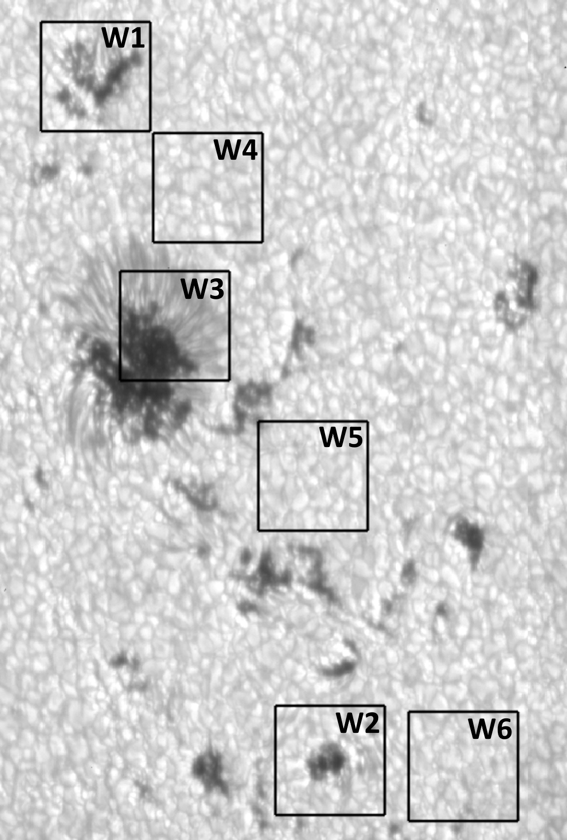
Since the observations from the space are not disturbed by the atmosphere, as the reference data for our experiments we used the images obtained by the SOT. From a wide range of registered images in Hindoe database, we selected a one which contained several regions of enhanced magnetic activity (sunspots). The image was originally obtained at green continuum wavelength, on 29 Nov. 2015 at 21:19:44UT. In the Fig. allSun we show the selected reference and indicate the positions of six extracted $100\times 100$-pixel patches, (roughly $5^{\prime\prime}\times 5^{\prime\prime}$ each, image scale of 0.054” pixel^-1). Patches W1, W2, and W3 include sunspots, while W4, W5, and W6 contain granulation.

Figure 1.: A part of solar photosphere imaged by the Hindoe satellite. The six patches, ($W1-W6$, $100\times 100$ pixels) extracted for the experiment, are annotated. Three of them ($W1,W2,W3$) contain the parts of active regions, while the remaining ones ($W4,W5,W6$) include only granulation. The image was obtained in the green continuum on 29 Nov. 2015 at 21:19:44 UT.allSun

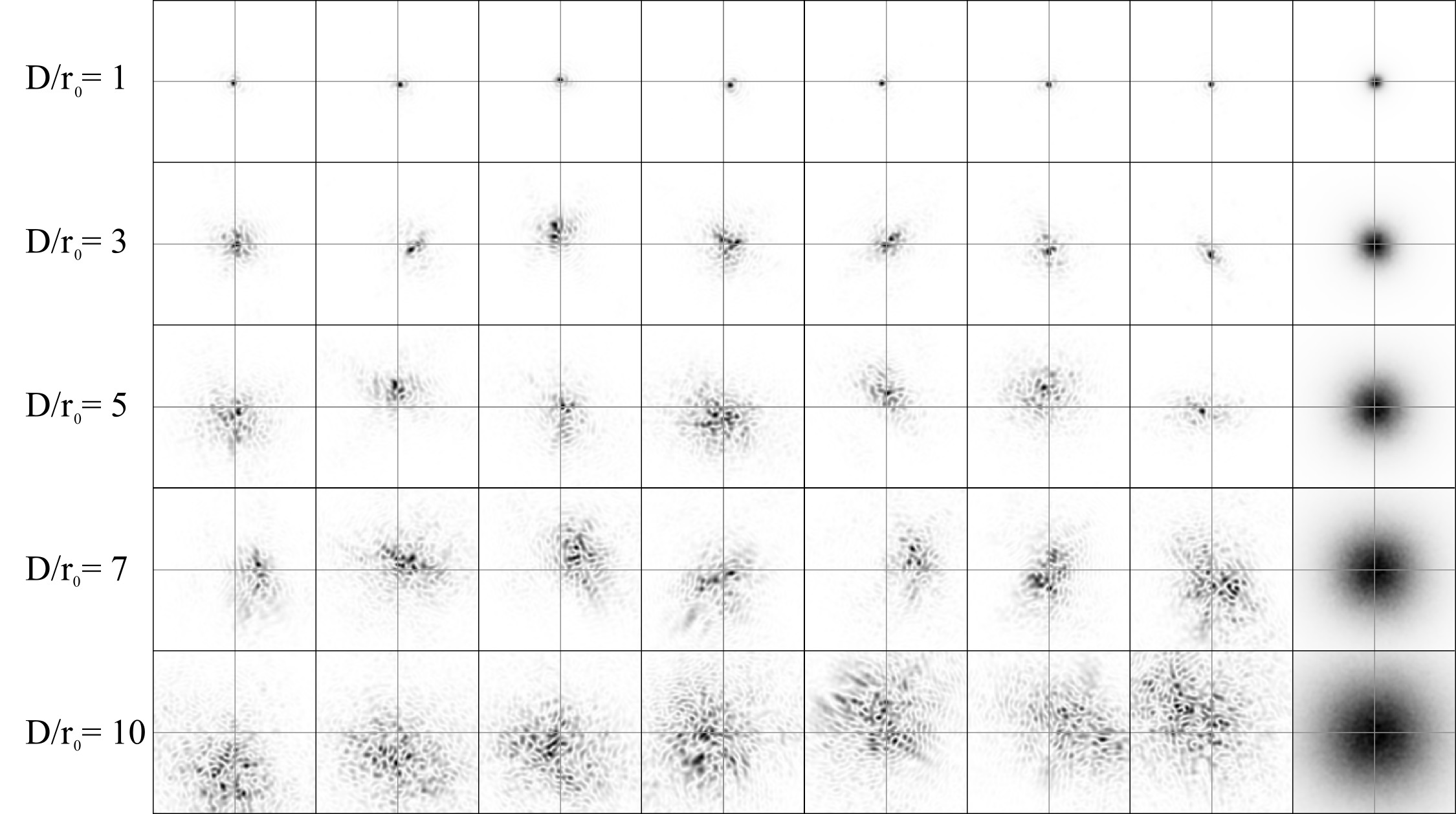
To investigate the response of various QMs for a given strength of turbulence, we modeled the transfer function of the atmosphere utilizing RWV method. The method allows for reliable modeling of amplitude and phase fluctuations of the incoming optical wavefront. Since a patch of solar photosphere, which is used for quality assessment, can be arbitrarily small we assumed that it is within the isoplanatic angle. Thus, anisoplanatic effects, more complicated for simulation, are neglected in this study, which will otherwise significantly complicate the simulations. Using RVW we generated 1000 blurring kernels (speckles patterns) for ten distinctive scenarios of seeing conditions: $D/r_{0}$ = 1, 2, …, 10. We assumed that such a range is representative for observations at best observing sites. Each generated kernel consisted of 1024$\times$1024 pixels and the resolution was two times higher than required by the Nyquist limit, i.e, a single pixel corresponded to an angular size of $\lambda/4D$ ($\lambda$ – wavelength, $D$ – telescope diameter). We opted for such oversampling to be able to combine simulated speckle kernels with reference Hindoe images. Each blurring kernel was normalized so that the summed intensity over all pixels is unity. Exemplary kernels with the corresponding long-exposure seeing disks are presented in Fig. kernels1. Evidently, the poorer the seeing conditions (higher $D/r_{0}$), the more complex is the kernel shape. The simulated tip-tilt effect is also visible as a displacement of the kernel’s centroid.

Figure 2.: Exemplary blurring kernels (negatives) employed in the experiment. The rows correspond to various $D/r_{0}$ relative atmospheric conditions while the last column exposes the simulated long-exposure seeing disk (i.e., an ensemble average over all the kernels for a given $D/r_{0}$). Each kernel is presented in a box with a side length of $40\lambda/D$. The auxiliary gray lines indicate the box center highlighting the simulated tip-tilt effect.kernels1

Atmospheric scintillation results in varying attenuation of flux collected by a telescope. This type of noise was recently investigated by Osborn et al. (2015). The authors present the following formula for estimating the relative variance of the total intensity of the observed object:

$$\sigma_{s}=\sqrt{10^{-5}~{}C^{2}_{Y}~{}D^{-4/3}~{}t_{e}^{-1}~{}(\textrm{cos}\gamma)^{-3}~{}\textrm{exp}(-2h_{\mathrm{obs}}/H)},$$ (1)

where $D$ is telescope diameter, $\gamma$ is the zenith distance , $h_{\mathrm{obs}}$ is the altitude of the observatory, $H$ is the scale height of the atmospheric turbulence, generally assumed to be $\sim$ 8000 m, $C_{Y}$ is the scaling coefficient which can be determined from turbulence profilers (SCIDARs) and was estimated between 1.30$-$1.67 for best observing sites (see Tab. 1 in the original work Osborn et al. (2015)).

To include such fluctuations in our simulated images, we multiplied each kernel by a random variable with an expected value of unity and a standard deviation equal to $\sigma_{s}$. We assumed (1) the telescope size $D=0.5$ m according to the size of Hindoe/SOT instrument, (2) the observations at zenith distance of $\gamma=60^{\circ}$ and (3) a low scintillation index, $C_{y}=1.5$, which is expected for (4) high-altitude observatory, $h_{\mathrm{obs}}=3000$ m. For such conditions the relative scintillation noise is $\sigma_{s}=0.032$.

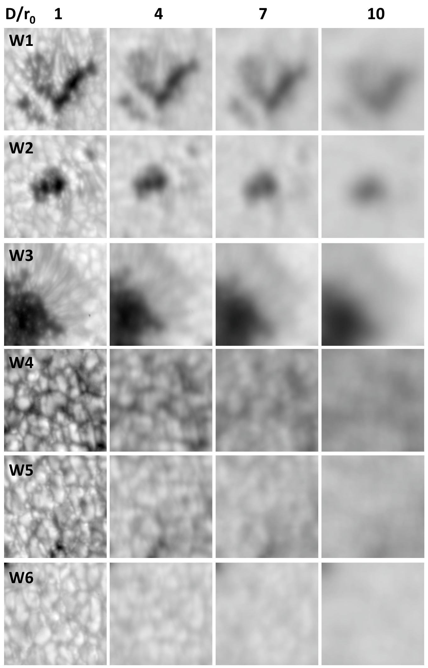
To properly convolve a blurring kernel with a reference patch, the scale of a kernel has to be the same as the image scale. For the assumptions given above, i.e., $D=0.5$ m telescope observing at $\lambda=550$ nm, we obtain an image scale of 0.055” pixel^-1. This means that the sampling of blurring kernels ($D/4\lambda$) and the assumed telescope size allow for convolving kernels with the Hindoe images without any prescalling. Several examples of solar images degraded by simulated blurring kernels are presented in Fig. patches1.

Figure 3.: Exemplary simulated images for all six patches (rows) and four selected degrees of atmospherics turbulence, $D/r_{0}=1,~{}4,~{}7,\textrm{~{}and~{}}10$ (columns).patches1

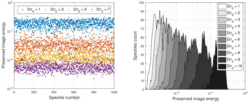
The time-dependent quality, when observing stellar objects, can be determined from the relative intensity of the brightest pixel in the normalized kernel. This is a widely accepted approach to select the sharpest frames in the nighttime lucky imaging (Law, Mackay, and Baldwin, 2006). However, in our case the object is not point-like and shows complex structures. Thus, we decided to use the quality measure based on the amount of energy preserved from the original frequency spectrum. Since the original image is convolved with a blurring kernel and the original amplitudes in frequency spectrum are multiplied by the amplitudes of a kernel, the value of proposed quality measure can be calculated by summing squared amplitudes in 2-D Fourier transform of a kernel. According to the Parseval’s theorem, this also equals to the sum of squared intensities of a kernel directly in the image plane.

Since turbulence is a random process, there is also a possibility that the temporal seeing conditions will become much better or much worse than the ones indicated by the average $D/r_{0}$ (Fried, 1978). This is in fact what we also observed in our data. For all ten sets of simulated kernels ($D/r_{0}=1,2,...,10$), the spread of temporal quality is exposed in the histograms in Fig. qKernel. In the upper part of Fig. qKernel we plotted the amount of preserved energy of the original image over all 1000 kernels for three values of $D/r_{0}$. Clearly, the quality for the average $D/r_{0}=4$ can sometimes outperform the conditions registered at $D/r_{0}=1$. Therefore, $D/r_{0}$ expresses only the average blurring strength while it can not be taken as a reliable estimator of the quality of individual frames.

Figure 4.: Dependencies of temporal turbulence strength expressed by the maximal intensity in normalized blurring kernel, on the average seeing conditions $D/r_{0}$. Left: amount of preserved image energy for three 1000-kernel sets $D/r_{0}=1,4$, and 10. Rigth: histograms of the preserved image energy over all the simulated kernels. (Color figures are available in online version.)qKernel

2.2 Methods

A set of 35 state-of-the-art QMs was provided in the review of Pertuz, Puig, and Garcia (2013). The authors consider the most popular methods dedicated for the assessment of focus in complex scenes by means of contrast measurement. The methods can be categorized into six families of operators, based on: gradients (GRA), Laplacians (LAP), wavelets (WAV), intensity statistics (STA), discrete-cosine transform (DCT), and the miscellaneous methods (MIS), i.e., the ones that can not be categorized into any other group. An overview of the methods with their abbreviations and references is given in Tab. tab_par_ref.

Within the set of techniques one can find the most popular method used in solar image processing, i.e., rms-contrast measure, which was called Normalized Gray-level Variance and abbreviated as STA5 (we followed this nomenclature). The most recent QM proposed by Deng et al. (2015), Median Filter Gradient Similarity (GRA8), was included in our comparison as well.

Table 1.: Overview of quality measures.

Abbr.	Operator name	Citation
Miscellaneous operators (MIS*)
MIS1	Absolute Central Moment	Shirvaikar (2004)
MIS2	Brenner’s Focus measure	Brenner et al. (1976)
MIS3	Image Contrast	Nanda and Cutler (2001)
MIS4	Image Curvature measure	Helmli and Scherer (2001)
MIS5	Helmli and Scherer’s Mean	Helmli and Scherer (2001)
MIS6	Local Binary Patterns measure	Lorenzo et al. (2008)
MIS7	Steerable Filters-based measure	Minhas et al. (2009)
MIS8	Spatial Frequency measure	Malik and Choi (2008)
MIS9	Vollath’s Autocorrelation	Vollath (1987)
Gradient-based operators (GRA*)
GRA1	Gaussian Derivative	Geusebroek et al. (2000)
GRA2	Gradient Energy	Subbarao, Choi, and Nikzad (1993)
GRA3	Thresholded Gradient	Santos (1997); Chern, Neow, and Ang (2001)
GRA4	Squared Gradient	Geusebroek et al. (2000)
GRA5	3D Gradient	Ahmad and Choi (2007)
GRA6	Tenengrad	Tenenbaum (1971); Schlag et al. (1983)
GRA7	Tenengrad Variance	Pech-Pacheco et al. (2000)
GRA8	Median Filter Gradient Similarity	Deng et al. (2015)
Laplacian-based operators (LAP*)
LAP1	Energy of Laplacian	Subbarao, Choi, and Nikzad (1993)
LAP2	Modified Laplacian	Nayar and Nakagawa (1994)
LAP3	Diagonal Laplacian	Thelen et al. (2009)
LAP4	Variance of Laplacian	Pech-Pacheco et al. (2000)
Wavelet-based operators (WAV*)
WAV1	Sum of Wavelet Coefficients	Yang and Nelson (2003)
WAV2	Variance of Wavelet Coefficients	Yang and Nelson (2003)
WAV3	Ratio of Wavelet Coefficients	Xie, Rong, and Sun (2006)
WAV4	Ratio of Curvelet Coefficients	Minhas et al. (2009)
Statistics-based operators (STA*)
STA1	Chebyshev Moments-based	Yap and Raveendran (2004)
STA2	Eigenvalues-based	Wee and Paramesran (2007)
STA3	Gray-level Variance	Groen, Young, and Ligthart (1985)
STA4	Gray-level Local Variance	Pech-Pacheco et al. (2000)
STA5	Normalized Gray-level Variance	Groen, Young, and Ligthart (1985)
STA6	Modified Gray-level Variance	Pertuz, Puig, and Garcia (2013)
STA7	Histogram Entropy	Firestone et al. (1991)
STA8	Histogram Range	Firestone et al. (1991)
DCT-based operators (DCT*)
DCT1	DCT Energy Ratio	Shen and Chen (2006)
DCT2	DCT Reduced Energy Ratio	Lee et al. (2009)
DCT3	Modified DCT	Lee et al. (2008)

tab_par_ref

To improve the effectiveness of QMs for solar observations we had to adjust the parameters of many techniques. This was carried out experimentally by tuning the parameter considering the properties of observed solar scene and analyzing the algorithm’s details. Moreover, for some of the methods we proposed major, but still simple, modifications which allowed for enhancing their effectiveness. This resulted in creation of various implementations of the most of methods (labeled as version $A$, $B$, etc.). The set of investigated parameter values and/or the details of applied modifications are given in Tab. method_params. The distance parameters, like radius or size of local filtering window, are expressed in pixels (in our case 1 pixel = 0.055”). The thresholds are given in relative values, which means that before applying thresholding the intensities in a patch were normalized such that the intensities cover the range from zero to unity. Several methods have two adjustable parameters, therefore we evaluated various combinations of their values. Including all the modifications, we end up in a total number of 105 implementations of 36 techniques which are included in our comparison.

Table 2.: The parameters and modifications of the quality measures compared in the experiment. Some methods do not have any parameters, thus they were left blank.method˙params

Method	Variants	Description
Miscellaneous operators (MIS*)
MIS1	A$-$D	number of bins in a histogram of image intensities ($L$)
		$L=\{50,100,256,1000\}$
MIS2	A	only horizontal gradient
	B	only vertical gradient
	C	maximum of vertical and horizontal gradients
	D$-$G	sum of vertical and horizontal gradients with thresholding ($T$)
		$T=\{0,0.01,0.1,0.5\}$
MIS3	–	–
MIS4	–	–
MIS5	A$-$C	window size ($w$)
		$w=\{3,7,15\}$
MIS6	A$-$D	radius of the circle in LBP operator ($r$)
		number of equally spaced pixels on the circle ($n$)
		$(r,n)=\{(1,8),(1,16),(2,8),(2,16)\}$
MIS7	A$-$H	size of the Gaussian mask ($N$)
		standard deviation of the Gaussian ($\sigma$)
		$(N,\sigma)=\{(7,2),(7,5),(7,10),(7,15),(15,2),(15,5),$
		$(15,10),(15,15)\}$
MIS8$-$9	–	–
Gradient-based operators (GRA*)
GRA1	A$-$F	size of Gaussian mask ($N$)
		standard deviation of the Gaussian ($\sigma$)
		$(N,\sigma)=\{(7,2),(7,5),(7,10),(15,2),(15,5),(15,10)\}$
GRA2	–	–
GRA3	A	maximum of the horizontal and vertical gradients
	B$-$F	horizontal gradient bigger than a threshold ($T$)
		$T=\{0.0,0.01,0.05,0.1,0.5\}$
	G$-$K	horizontal and vertical gradients bigger than a threshold ($T$)
		$T=\{0.0,0.01,0.05,0.1,0.5\}$
GRA4$-$7	–	–
GRA8	A	horizontal gradient and constant window size ($w$=3)
GRA8	B	vertical gradient and constant window size ($w$=3)
GRA8	C$-$F	horizontal and vertical gradient and window size $w$
		$w=\{3,5,7,11\}$
Laplacian-based operators (LAP*)
LAP1$-$4	–	–
Wavelet-based operators (WAV*)
WAV1	A	1-level DWT with Daubechies-6 filters
	B	2-level DWT and Daubechies-10 filters
WAV2	A	1-level DWT with Daubechies-6 filters
	B	2-level DWT and Daubechies-10 filters
WAV3$-$4	–	–

Table 3.: Continuation of Tab. method_paramsmethod˙params2

Method	Variants	Description
Statistics-based operators (STA*)
STA1	A$-$E	order of Tchebichef polynomials ($p$)
		$p=\{2,3,4,5,6\}$
STA2	A$-$E	number of diagonal elements from the matrix of eigenvalues ($k$)
		$k=\{1,3,5,7,9\}$
STA3	–	–
STA4	A$-$E	size of the window in which the local variance is computed ($w$)
		$w=\{3,5,7,11,15\}$
STA5	–	–
STA6	A$-$E	size of the window in which the local mean is computed ($w$)
		$w=\{3,5,7,11,15\}$
STA7	A$-$D	number of bins in histogram of image intensities ($L$)
		$L=\{50,100,256,1000\}$
STA8	A$-$D	percent of pixels removed from the histogram ($\alpha$)
		$\alpha=\{0,0.01,0.02,0.05\}$
DCT-based operators (DCT*)
DCT1	A$-$C	size of sub-block of the image
		$w=\{4,8,16\}$
DCT2	A$-$C	size of sub-block of the image
		$w=\{4,8,16\}$
DCT3	–	–

2.3 Data analysis

To assess the performance of all methods we investigated the correlation between the results of QMs and the actual expected quality $Q$. As stated before, the quality was estimated by the total preserved energy with respect to the reference, undisturbed image. We observed that the relation between these two quantities is almost always nonlinear. Fortunately, it is sufficient that the dependency is monotonic as it allows us to distinguish between better and worse atmospheric conditions. Therefore, to estimate the effectiveness of the methods, instead of Pearson’s correlation coefficient, we used the Spearman rank-order correlation $C_{s}$. Such a coefficient is insensitive to any nonlinearities in observed dependencies.

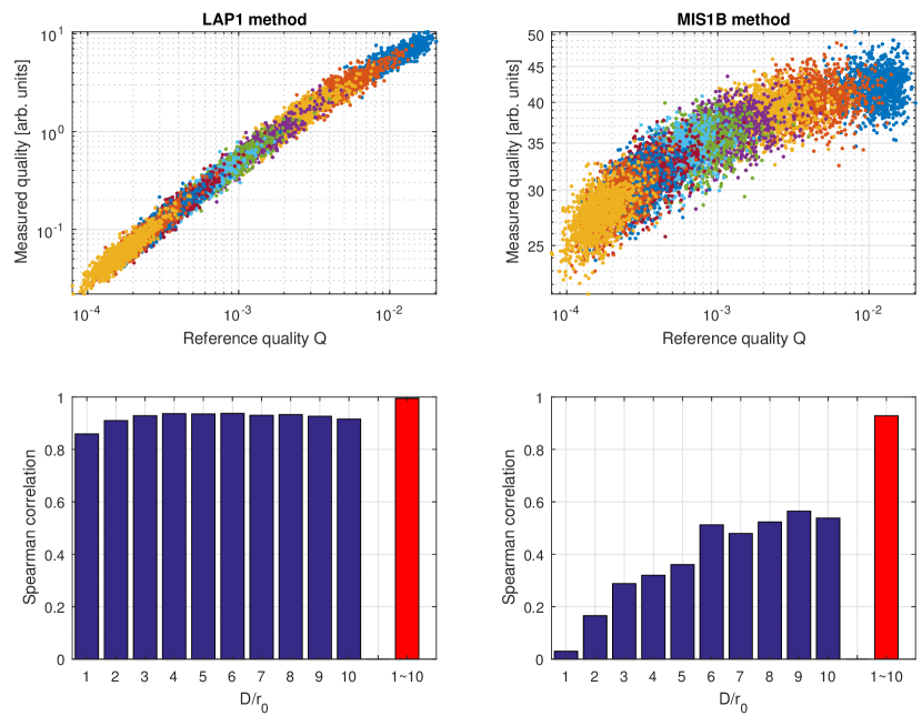
As an example in the upper panel of Fig. corrExamples we show significantly different dependencies between the expected quality Q and the outcomes of two QMs (LAP1 and MISB, on the left and right side, respectively) calculated for image patch $W1$. Each set of $D/r_{0}$ was presented with a different marker/color. We decided to calculate the Spearman correlation coefficient in two ways: (1) within a set of observations for each $D/r_{0}$ and (2) across all the simulated conditions $D/r_{0}=1-10$. We present the corresponding results of $C_{s}$ in each $D/r_{0}$ subset in the bar plots of Fig. corrExamples. The correlation depends on $D/r_{0}$ so that it becomes apparent which range of atmospheric conditions is most suitable for a given method. For example, the LAP1 method allows for effective estimation of image quality in $D/r_{0}=1$ while MIS1B is completely useless in this range. The proposed approach to calculate the correlation coefficient permitted estimating the performance of each method for a range of typical atmospheric conditions.

In the example presented in Fig. corrExamples the superiority of LAP1 over MIS1B is also visible for $C_{s}$ calculated over whole set of $D/r_{0}$. However, the difference is significantly smaller than in particular groups as both methods achieve $C_{s}>0.9$ (0.98 and 0.90 for LAP1 and MIS1B, respectively). This is due to the wide range of considered $Q$ values, which makes the correlation between the quantities more evident and leads to the elevated value of the $C_{s}$ coefficient. Although the differences are not so significant, the correlation for such a wide range of $Q$ values still allows for comparison of the overall effectiveness of QMs, however, within much narrower range of $C_{s}$ values.

Figure 5.: Examples of correlation between measured and expected image quality for two distinct methods: LAP1 – left side and MIS1B – right side. The analysis was performed for image patch W1. The calculated correlation coefficients in each $D/r_{0}$ set and over whole data set ($D/r_{0}=1-10$) are presented in the lower bar plots. Colors in point correspond to various $D/r_{0}$ conditions. (Color figures are available in online version.)corrExamples

2.4 Results and discussion

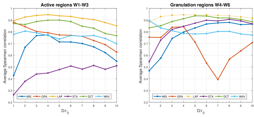
The results of the comparison are presented in Tab. tab_wyniki and Fig. families. While in Tab. tab_wyniki we present only the best four methods for each $D/r_{0}$, the average performance obtained for whole QM families is summarized in Fig. families. We divided the results into two categories, according to the contents of observed image: W1, W2, and W3 – active regions, and W4, W5, and W6 – granulation.

Table 4.: The rankings of best quality measures for various $D/r_{0}$ seeing conditions and six analyzed patches: W1, W2, W3 – active regions and W4, W5, W6 – granulation areas. The lower bar plots show the rankings for wide-range correlation accross all atmospheric conditions $D/r_{0}=1-10$.

		$D/r_{0}=1$	$D/r_{0}=2$	$D/r_{0}=3$	$D/r_{0}=4$	$D/r_{0}=5$
W1–W3	active regions
W4–W6	granulation
		$D/r_{0}=6$	$D/r_{0}=7$	$D/r_{0}=8$	$D/r_{0}=9$	$D/r_{0}=10$
W1–W3	active regions
W4–W6	granulation

$D/r_{0}=1-10$
W1–W3	W4–W6
active regions	granulation

tab_wyniki

Figure 6.: Average correlation coefficients obtained for QM families. The left panel corresponds to the results for active regions, while the right one shows outcomes for granulation patches. (Color figures are available in online version.)families

According to the results presented in Tab. tab_wyniki, there is no single winner covering all possible atmospherics conditions and scene characteristics. However, there are three techniques which showed distinctively better performance and, therefore, they are discussed below.

One of the methods with very impressive performance, is Helmli and Scherer’s Mean method (MIS5) proposed by Helmli and Scherer (2001). This technique provided very good results for whole range of $D/r_{0}$ conditions and both types of observed solar regions. For all atmospheric conditions it is always among the four best methods. As indicated by distinctively higher correlation coefficients calculated over $D/r_{0}=1-10$, its usefulness should be considered when the seeing is highly varying or unknown. In summary, this method should be the first choice among all tested techniques.

The second noteworthy method is the Median Filter Gradient Similarity (GRA8) method, which was recently proposed by Deng et al. (2015). It shows the best performance for very good atmospherics conditions ($D/r_{0}<4$). However, to achieve the high effectiveness we had to slightly modify the method by (1) combining both horizontal and vertical gradients and (2) changing the size of kernel. The superiority of the method is evident especially for active regions (W1$-$W3), while it is slightly less efficient when assessing only granulation patches (W4$-$W6), especially for $D/r_{0}>2$. Interestingly, this technique was not included in the best 12 methods indicated by wide-range correlations, $D/r_{0}=1-10$ which indicates that it should not be applied for observations with poor or unknown atmospherics conditions. The results of the GRA8 method recommend it for the utilization in observations assisted by AO since in this case the image quality is significantly enhanced, and the effective $D/r_{0}$ is small.

The last method, which provides good results is the DCT Energy Ratio proposed by Shen and Chen (2006). Its performance is the highest for moderate and poor atmospherics conditions when observing granulation regions. This method is second best method when the whole range of $D/r_{0}$ is taken into account, for patches W4-W6. The parameter of this method - the size of sub-block - should be selected accordingly to the blurring strength, i.e., the larger the $D/r_{0}$, the larger the sub-block.

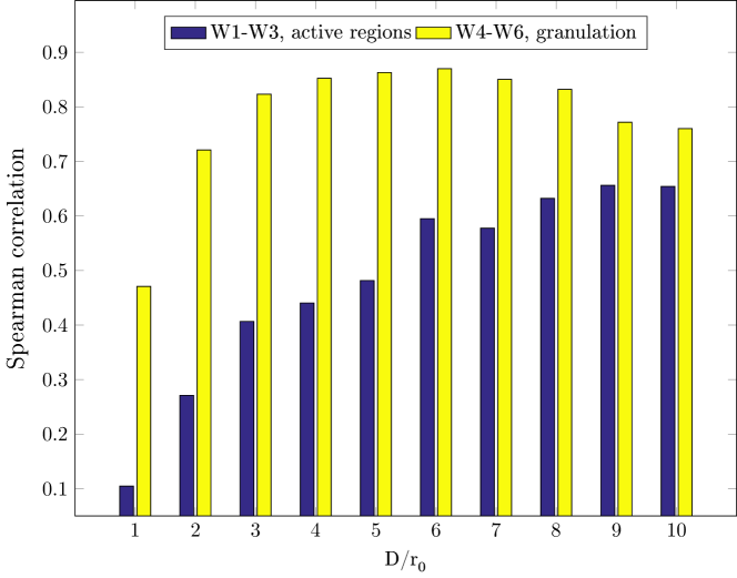
The method frequently used in solar observations, rms-contrast or normalized gray-level variance (STA5), showed surprisingly poor performance. Since the rms-contrast measure was originally developed for granulation regions, with isotropic and uniform characteristics, we investigated how the method performed for this type of scene. The results presented in Fig. rms_test indicate that indeed the techniques allows for achieving significantly higher correlation values for granulation. Still, the outcomes based on rms-contrast were much less correlated with the expected image quality than the results achieved by the best techniques. Therefore, it did not appeared in any ranking presented in Tab. tab_wyniki. Our conclusions agree with the observations made by Deng et al. (2015) who also indicate relatively low efficiency of the common rms-contrast measure.

Figure 7.: Comparison of the effectiveness of most popular image quality technique used for solar images, i.e., rms-contrast. Significantly higher correlation values are achieved for granulation regions. rms˙test

Some interesting conclusions can be drawn from the average performance of each QM family presented in Fig. families. The Laplacian-based methods (LAP) show very good average correlation with $D/r_{0}$ for both types of observed scenes. While the LAP-based methods are indicated only several times in the rankings presented in Tab. tab_wyniki, they still should be considered as a base for new, better techniques. The biggest difference between the efficiency when changing from granulation to active regions, can be observed in statistical methods (STA). This agrees well with the results shown in Fig. rms_test and appears due to the assumption made in STA methods that regions should expose uniform properties across the observed field. The strange shape of GRA dependency visible in the right plot of Fig. families arises due to the characteristics of Median Filter Gradient Similarity (GRA8). As it was stated before, the performance of this method rises significantly as the $D/r_{0}$ decrease. This behavior biases the average efficiency of GRA family.

The possibility of using a method in real-time image selection can be especially important, as it allows for recording only the most useful data. Therefore, for completeness of our comparison, we measured the time required for processing a single image patch by each method. The evaluations were performed on a single core of IntelCore i7-3930K operating at 3.2 Ghz. The procedures were repeated $10^{4}$ times to obtain the average execution time. The results are presented in Tab. tab_times wherein we show the methods and their average computation time (single-image analysis) in seconds, alternately.

The results show that real-time frame selection for the assumed size of image patch is possible for frame rates more than 1000fps for most of the analyzed methods. This can be, however, not true if one wants to process large, full resolution, frames and/or if several steps of image calibration have to be applied. For such a case, the usage of graphics processing units (GPU) and accompanying optimization of a code should be considered. However, in our comparison we decided to perform measurements on a single CPU core, so that the further reduction of execution time with a multi-core machine can be estimated. For most of the included methods, the analysis is performed independently in local sub-regions of whole image, which makes them easily parallelized.

We observed that the Median Filter Gradient Similarity (GRA8) requires visibly more computation time ($>$0.01 s) than MIS5 ($<$0.002 s). It is mostly due to the median filtering which requires sorting pixels in a sliding window. This indicates that GRA8, compared to MIS5, would require more computing resources and/or better code optimization to operate at high frame rates utilized frequently in solar observations. Unfortunately, the Discrete Cosine Transform techniques (DCT1 and DCT2) have significantly higher execution time, which makes them useless for real-time computation. These methods should be considered only in the post-processing. The fastest method was the one most frequently utilized in solar observations, STA5. Unfortunately its mediocre performance is not compensated by the distinctively higher computational efficiency.

Table 5.: Computation efficiency of the methods. In each consecutive column we show method abbreviation and execution time in seconds, alternately. The three fastest methods are indicated in bold.

MIS1A	0.0020	MIS7H	0.0114	GRA8C	0.0388	STA6C	0.0026
MIS1B	0.0025	MIS8	0.0011	GRA8D	0.0752	STA6D	0.0021
MIS1C	0.0029	MIS9	0.0013	GRA8E	0.0082	STA6E	0.0023
MIS1D	0.0039	GRA1A	0.0050	GRA8F	0.0081	STA7A	0.0013
MIS2A	0.0010	GRA1B	0.0041	LAP1	0.0017	STA7B	0.0018
MIS2B	0.0011	GRA1C	0.0038	LAP2	0.0027	STA7C	0.0031
MIS2C	0.0006	GRA1D	0.0050	LAP3	0.0039	STA7D	0.0046
MIS2D	0.0023	GRA1E	0.0046	LAP4	0.0014	STA8A	0.0006
MIS2E	0.0024	GRA1F	0.0044	STA1A	0.0012	STA8B	0.0021
MIS2F	0.0026	GRA2	0.0012	STA1B	0.0012	STA8C	0.0022
MIS2G	0.0017	GRA3A	0.0009	STA1C	0.0012	STA8D	0.0020
MIS3	0.0160	GRA3B	0.0012	STA1D	0.0012	DCT1A	7.8562
MIS4	0.0065	GRA3C	0.0013	STA1E	0.0012	DCT1B	6.5742
MIS5A	0.0028	GRA3D	0.0013	STA2A	0.0060	DCT1C	8.0760
MIS5B	0.0031	GRA3E	0.0011	STA2B	0.0058	DCT2A	5.5642
MIS5C	0.0027	GRA3F	0.0010	STA2C	0.0058	DCT2B	5.7970
MIS6A	0.0768	GRA3G	0.0020	STA2D	0.0056	DCT2C	7.7149
MIS6B	0.0855	GRA3H	0.0021	STA2E	0.0058	DCT3	0.0011
MIS6C	0.0806	GRA3I	0.0025	STA3	0.0010	WAV1A	0.0099
MIS6D	0.0809	GRA3J	0.0019	STA4A	0.0037	WAV1B	0.0143
MIS7A	0.0135	GRA3K	0.0021	STA4B	0.0040	WAV2A	0.0105
MIS7B	0.0136	GRA4	0.0011	STA4C	0.0047	WAV2B	0.0150
MIS7C	0.0141	GRA5	0.0079	STA4D	0.0036	WAV3	0.0265
MIS7D	0.0129	GRA6	0.0030	STA4E	0.0045	WAVC	0.0848
MIS7E	0.0107	GRA7	0.0023	STA5	0.0005
MIS7F	0.0108	GRA8A	0.0072	STA6A	0.0019
MIS7G	0.0106	GRA8B	0.0204	STA6B	0.0016

tab_times

3 Conclusions

The assessment of image quality is an integral part of observations of the solar photosphere and chromosphere. It is essential to precisely select only the images of the highest fidelity before performing consecutive image reconstruction. Unfortunately the complexity and variety of observed structures make the estimation of image quality a challenging task. There is no single point-like object available, therefore, the selection techniques utilized in nighttime lucky imaging are not applicable.

In this study we decided to employ 36 techniques with various implementations and evaluated their precision in selecting the best exposures. The methods were based on various principles (gradients, intensity statistics, wavelets, Laplacians, Discrete Cosine Transforms) and were published over the last 40 years. Additionally, we enhanced their performance by applying simple modifications and by adjusting their tunable parameters.

In the comparison we employed reference images, containing both active regions and granulation areas, obtained by the Hidnoe satellite. The selected patches were degraded by convolution with blurring kernels generated by RWV method which faithfully reflects the seeing characteristics. We assumed a wide range of relative atmospheric conditions, starting from nearly undisturbed observations at $D/r_{0}=1$ to mediocre seeing at $D/r_{0}=10$. The reference quality of each simulated image was objectively estimated by measuring the amount of energy preserved in the Fourier spectrum of the original image. Eventually, to assess the efficiency of the compared techniques, we calculated Spearman’s correlation coefficient between the outcomes of each method and the expected image quality.

The results of our comparison showed that the efficiency depends on the strength of atmospheric turbulence. For good seeing, $D/r_{0}<4$, the best method is the Median Filter Gradient Similarity (Deng et al., 2015), (GRA8), the most recent technique proposed for solar observations. Importantly, the original idea had to be slightly modified to enhance the method’s performance. On the other hand, when the seeing conditions cover a wide range, the most efficient method is the Helmli and Scherer’s Mean (Helmli and Scherer, 2001), (MIS5). This method should be considered when observing without AO or if the seeing conditions are unknown. The last distinctive method was the DCT Energy Ratio (Shen and Chen, 2006) which showed high performance in poor atmospheric conditions when observing granulation regions. The measurements of execution time indicated that of the three mentioned techniques the Helmli and Scherer’s Mean has significantly higher computational efficiency which recommends it for utilization with extremely high frame rates and/or larger image patches.

Acknowledgments

We would like to thank for numerous important comments, thorough review and great help in polishing the English provided by the anonymous Reviewer. This research was supported by the Polish National Science Centre grants 2016/21/D/ST9/00656 and (A. Popowicz) and 2015/17/N/ST7/03720 (K. Bernacki). We would like also to acknowledge the support from Polish Ministry of Science and Higher Education funding for statutory activities.

References

- Ahmad and Choi (2007) Ahmad, M.B., Choi, T.S.: 2007, Application of three dimensional shape from image focus in lcd/tft displays manufacturing. IEEE Transactions on Consumer Electronics 53(1), 1. DOI.
- Albregtsen and Hansen (1977) Albregtsen, F., Hansen, T.L.: 1977, The wavelength dependence of granulation /0.38-2.4 microns/. Sol. Phys. 54, 31. DOI. ADS.
- Beckers (1989) Beckers, J.M.: 1989, Improving solar image quality by image selection. In: Rutten, R.J., Severino, G. (eds.) NATO Advanced Science Institutes (ASI) Series C, NATO Advanced Science Institutes (ASI) Series C 263, 55. ADS.
- Brenner et al. (1976) Brenner, J.F., Dew, B.S., Horton, J.B., King, T., Neurath, P.W., Selles, W.D.: 1976, An automated microscope for cytologic research a preliminary evaluation. Journal of Histochemistry & Cytochemistry 24(1), 100. PMID: 1254907. DOI. http://dx.doi.org/10.1177/24.1.1254907.
- Chern, Neow, and Ang (2001) Chern, N.N.K., Neow, P.A., Ang, M.H.: 2001, Practical issues in pixel-based autofocusing for machine vision. In: Proceedings of IEEE International Conference on Robotics and Automation 3, 2791. DOI.
- Colodro-Conde et al. (2017) Colodro-Conde, C., Velasco, S., Fernández-Valdivia, J.J., López, R., Oscoz, A., Rebolo, R., Femenía, B., King, D.L., Labadie, L., Mackay, C., Muthusubramanian, B., Pérez Garrido, A., Puga, M., Rodríguez-Coira, G., Rodríguez-Ramos, L.F., Rodríguez-Ramos, J.M., Toledo-Moreo, R., Villó-Pérez, I.: 2017, Laboratory and telescope demonstration of the TP3-WFS for the adaptive optics segment of AOLI. MNRAS 467, 2855. DOI. ADS.
- Danilovic et al. (2008) Danilovic, S., Gandorfer, A., Lagg, A., Schüssler, M., Solanki, S.K., Vögler, A., Katsukawa, Y., Tsuneta, S.: 2008, The intensity contrast of solar granulation: comparing Hinode SP results with MHD simulations. A&A 484, L17. DOI. ADS.
- Deng et al. (2015) Deng, H., Zhang, D., Wang, T., Ji, K., Wang, F., Liu, Z., Xiang, Y., Jin, Z., Cao, W.: 2015, Objective image-quality assessment for high-resolution photospheric images by Median Filter-Gradient Similarity. Sol. Phys. 290, 1479. DOI. ADS.
- Denker et al. (2005) Denker, C., Mascarinas, D., Xu, Y., Cao, W., Yang, G., Wang, H., Goode, P.R., Rimmele, T.: 2005, High-spatial-resolution imaging combining high-order adaptive optics, frame selection, and speckle masking reconstruction. Solar Physics 227(2), 217. DOI. http://dx.doi.org/10.1007/s11207-005-1108-4.
- Ferayorni et al. (2016) Ferayorni, A., Beard, A., Cole, W., Gregory, S., Wöeger, F.: 2016, Bottom-up laboratory testing of the DKIST Visible Broadband Imager (VBI). In: Modeling, Systems Engineering, and Project Management for Astronomy VI, Proc. SPIE 9911, 991106. DOI. ADS.
- Firestone et al. (1991) Firestone, L., Cook, K., Culp, K., Talsania, N., Preston, K.: 1991, Comparison of autofocus methods for automated microscopy. Cytometry 12(3), 195. DOI. http://dx.doi.org/10.1002/cyto.990120302.
- Fried (1978) Fried, D.L.: 1978, Probability of getting a lucky short-exposure image through turbulence. Journal of the Optical Society of America (1917-1983) 68, 1651. ADS.
- Geusebroek et al. (2000) Geusebroek, J.-M., Cornelissen, F., Smeulders, A.W.M., Geerts, H.: 2000, Robust autofocusing in microscopy. Cytometry 39(1), 1. DOI. http://dx.doi.org/10.1002/(SICI)1097-0320(20000101)39:1¡1::AID-CYTO2¿3.0.CO;2-J.
- Groen, Young, and Ligthart (1985) Groen, F.C.A., Young, I.T., Ligthart, G.: 1985, A comparison of different focus functions for use in autofocus algorithms. Cytometry 6(2), 81. DOI. http://dx.doi.org/10.1002/cyto.990060202.
- Hardy (1998) Hardy, J.W.: 1998, Adaptive optics for astronomical telescopes, 448. ADS.
- Helmli and Scherer (2001) Helmli, F.S., Scherer, S.: 2001, Adaptive shape from focus with an error estimation in light microscopy. In: Proceedings of the 2nd International Symposium on Image and Signal Processing and Analysis. In conjunction with 23rd International Conference on Information Technology Interfaces, 188. DOI.
- Hofmann and Weigelt (1993) Hofmann, K.-H., Weigelt, G.: 1993, Iterative image reconstruction from the bispectrum. A&A 278, 328. ADS.
- Ireland (2013) Ireland, M.J.: 2013, Phase errors in diffraction-limited imaging: contrast limits for sparse aperture masking. MNRAS 433, 1718. DOI. ADS.
- Law, Mackay, and Baldwin (2006) Law, N.M., Mackay, C.D., Baldwin, J.E.: 2006, Lucky imaging: high angular resolution imaging in the visible from the ground. Astronomy and Astrophysics 446, 739. DOI. ADS.
- Lee et al. (2008) Lee, S.-Y., Kumar, Y., Cho, J.-M., Lee, S.-W., Kim, S.-W.: 2008, Enhanced autofocus algorithm using robust focus measure and fuzzy reasoning. IEEE Trans. Cir. and Sys. for Video Technol. 18(9), 1237. DOI. http://dx.doi.org/10.1109/TCSVT.2008.924105.
- Lee et al. (2009) Lee, S.Y., Yoo, J.T., Kumar, Y., Kim, S.W.: 2009, Reduced energy-ratio measure for robust autofocusing in digital camera. IEEE Signal Processing Letters 16(2), 133. DOI.
- Löfdahl (2010) Löfdahl, M.G.: 2010, Evaluation of image-shift measurement algorithms for solar Shack-Hartmann wavefront sensors. A&A 524, A90. DOI. ADS.
- Lohmann, Weigelt, and Wirnitzer (1983) Lohmann, A.W., Weigelt, G., Wirnitzer, B.: 1983, Speckle masking in astronomy - Triple correlation theory and applications. Applied Optics 22, 4028. DOI. ADS.
- Lorenzo et al. (2008) Lorenzo, J., Castrillon, M., Mendez, J., Deniz, O.: 2008, Exploring the use of local binary patterns as focus measure. In: Proceedings of International Conference on Computational Intelligence for Modelling Control Automation, 855. DOI.
- Mackay et al. (2012) Mackay, C., Rebolo-López, R., Castellá, B.F., Crass, J., King, D.L., Labadie, L., Aisher, P., Garrido, A.P., Balcells, M., Díaz-Sánchez, A., Fuensalida, J.J., Lopez, R.L., Oscoz, A., Pérez Prieto, J.A., Rodríguez-Ramos, L.F., Villó, I.: 2012, AOLI - Adaptive Optics Lucky Imager: diffraction limited imaging in the visible on large ground-based telescopes. In: Proceedings of SPIE 8446. DOI.
- Malik and Choi (2008) Malik, A.S., Choi, T.-S.: 2008, A novel algorithm for estimation of depth map using image focus for 3d shape recovery in the presence of noise. Pattern Recognition 41(7), 2200 . DOI. http://www.sciencedirect.com/science/article/pii/S0031320308000058.
- Minhas et al. (2009) Minhas, R., Mohammed, A.A., Wu, Q.M.J., Sid-Ahmed, M.A.: 2009, 3D shape from focus and depth map computation using steerable filters, Springer, Berlin, Heidelberg, 573. DOI. http://dx.doi.org/10.1007/978-3-642-02611-9˙57.
- Monnier et al. (2004) Monnier, J.D., Millan-Gabet, R., Tuthill, P.G., Traub, W.A., Carleton, N.P., Coudé du Foresto, V., Danchi, W.C., Lacasse, M.G., Morel, S., Perrin, G., Porro, I.L., Schloerb, F.P., Townes, C.H.: 2004, High-resolution imaging of dust shells by using keck aperture masking and the IOTA interferometer. ApJ 605, 436. DOI. ADS.
- Nanda and Cutler (2001) Nanda, H., Cutler, R.: 2001, Practical calibrations for a real-time digital omnidirectional camera. Technical report, In Technical Sketches, Computer Vision and Pattern Recognition.
- Nayar and Nakagawa (1994) Nayar, S.K., Nakagawa, Y.: 1994, Shape from focus. IEEE Transactions on Pattern Analysis and Machine Intelligence 16(8), 824.
- Osborn et al. (2015) Osborn, J., Föhring, D., Dhillon, V.S., Wilson, R.W.: 2015, Atmospheric scintillation in astronomical photometry. MNRAS 452, 1707. DOI. ADS.
- Pech-Pacheco et al. (2000) Pech-Pacheco, J.L., Cristobal, G., Chamorro-Martinez, J., Fernandez-Valdivia, J.: 2000, Diatom autofocusing in brightfield microscopy: a comparative study. In: Proceedings of 15th International Conference on Pattern Recognition 3, 314. DOI.
- Pertuz, Puig, and Garcia (2013) Pertuz, S., Puig, D., Garcia, M.A.: 2013, Analysis of focus measure operators for shape-from-focus. Pattern Recogn. 46(5), 1415. DOI. http://dx.doi.org/10.1016/j.patcog.2012.11.011.
- Rimmele (2004) Rimmele, T.R.: 2004, Recent advances in solar adaptive optics. In: Proceedings of SPIE 5490, 34. DOI.
- Rimmele and Marino (2011) Rimmele, T.R., Marino, J.: 2011, Solar adaptive optics. Living Reviews in Solar Physics 8, 2. DOI. ADS.
- Saha (2007) Saha, S.K.: 2007, Diffraction-limited imaging with large and moderate telescopes. DOI. ADS.
- Santos (1997) Santos, A.: 1997, Evaluation of autofocus functions in molecular cytogenetic analysis. Journal of Microscopy 188(3), 264. DOI. http://dx.doi.org/10.1046/j.1365-2818.1997.2630819.x.
- Scharmer (1989) Scharmer, G.B.: 1989, High resolution granulation observations from La Palma: Techniques and First Results. In: Rutten, R.J., Severino, G. (eds.) Solar and Stellar Granulation, NATO Adv. Sci. Inst. (ASI) Ser. C 263, 161.
- Scharmer et al. (2010) Scharmer, G.B., Löfdahl, M.G., van Werkhoven, T.I.M., de la Cruz Rodríguez, J.: 2010, High-order aberration compensation with multi-frame blind deconvolution and phase diversity image restoration techniques. A&A 521, A68. DOI. ADS.
- Schlag et al. (1983) Schlag, J.F., Sanderson, A.C., Neuman, C.P., Wimberly, F.C.: 1983, Implementation of automatic focusing algorithms for a computer vision system with camera control. Technical Report CMU-RI-TR-83-14, Robotics Institute, Pittsburgh, PA.
- Schödel and Girard (2012) Schödel, R., Girard, J.H.: 2012, Holographic imaging: a versatile tool for high angular resolution imaging. The Messenger 150, 26. ADS.
- Shen and Chen (2006) Shen, C.-H., Chen, H.H.: 2006, Robust focus measure for low-contrast images. In: 2006 Digest of Technical Papers International Conference on Consumer Electronics, 69. DOI.
- Shirvaikar (2004) Shirvaikar, M.V.: 2004, An optimal measure for camera focus and exposure. In: Proceedings of the Thirty-Sixth Southeastern Symposium on System Theory, 472. DOI.
- Socas-Navarro et al. (2005) Socas-Navarro, H., Beckers, J., Brandt, P., Briggs, J., Brown, T., Brown, W., Collados, M., Denker, C., Fletcher, S., Hegwer, S., Hill, F., Horst, T., Komsa, M., Kuhn, J., Lecinski, A., Lin, H., Oncley, S., Penn, M., Rimmele, T., Streander, K.: 2005, Solar site survey for the Advanced Technology Solar Telescope. I. Analysis of the Seeing Data. PASP 117, 1296. DOI. ADS.
- Subbarao, Choi, and Nikzad (1993) Subbarao, M., Choi, T.-S., Nikzad, A.: 1993, Focusing techniques. Optical Engineering 32(11), 2824. ISBN 0091-3286. DOI. http://dx.doi.org/10.1117/12.147706.
- Tenenbaum (1971) Tenenbaum, J.M.: 1971, Accommodation in computer vision. PhD thesis, Stanford, CA, USA.
- Thelen et al. (2009) Thelen, A., Frey, S., Hirsch, S., Hering, P.: 2009, Improvements in shape-from-focus for holographic reconstructions with regard to focus operators, neighborhood-size, and height value interpolation. IEEE Transactions on Image Processing 18(1), 151. DOI. http://dx.doi.org/10.1109/TIP.2008.2007049.
- Tokovinin and Cantarutti (2008) Tokovinin, A., Cantarutti, R.: 2008, First speckle interferometry at SOAR telescope with electron-multiplication CCD. PASP 120, 170. DOI. ADS.
- Tsuneta et al. (2008) Tsuneta, S., Ichimoto, K., Katsukawa, Y., Nagata, S., Otsubo, M., Shimizu, T., Suematsu, Y., Nakagiri, M., Noguchi, M., Tarbell, T., Title, A., Shine, R., Rosenberg, W., Hoffmann, C., Jurcevich, B., Kushner, G., Levay, M., Lites, B., Elmore, D., Matsushita, T., Kawaguchi, N., Saito, H., Mikami, I., Hill, L.D., Owens, J.K.: 2008, The Solar Optical Telescope for the Hinode Mission: An Overview. 249, 167. DOI.
- Voitsekhovich et al. (1999) Voitsekhovich, V.V., Kouznetsov, D., Orlov, V.G., Cuevas, S.: 1999, Method of random wave vectors in simulation of anisoplanatic effects. Appl. Opt. 38(19), 3985. DOI. http://ao.osa.org/abstract.cfm?URI=ao-38-19-3985.
- Vollath (1987) Vollath, D.: 1987, Automatic focusing by correlative methods. Journal of Microscopy 147(3), 279. DOI. http://dx.doi.org/10.1111/j.1365-2818.1987.tb02839.x.
- von der Lühe (1993) von der Lühe, O.: 1993, Speckle imaging of solar small scale structure. I - Methods. A&A 268, 374. ADS.
- Wee and Paramesran (2007) Wee, C.-Y., Paramesran, R.: 2007, Measure of image sharpness using eigenvalues. Information Sciences 177(12), 2533. DOI. http://www.sciencedirect.com/science/article/pii/S002002550700014X.
- Xie, Rong, and Sun (2006) Xie, H., Rong, W., Sun, L.: 2006, Wavelet-based focus measure and 3-d surface reconstruction method for microscopy images. In: 2006 IEEE/RSJ International Conference on Intelligent Robots and Systems, 229. DOI.
- Yang and Nelson (2003) Yang, G., Nelson, B.J.: 2003, Wavelet-based autofocusing and unsupervised segmentation of microscopic images. In: Proceedings 2003 IEEE/RSJ International Conference on Intelligent Robots and Systems (IROS 2003) (Cat. No.03CH37453) 3, 2143. DOI.
- Yap and Raveendran (2004) Yap, P.T., Raveendran, P.: 2004, Image focus measure based on chebyshev moments. IEE Proceedings - Vision, Image and Signal Processing 151(2), 128. DOI.