First Axion Dark Matter Search with Toroidal Geometry

Abstract

We report the first axion dark matter search with toroidal geometry. Exclusion limits of the axion-photon coupling $g_{a\gamma\gamma}$ over the axion mass range from 24.7 to 29.1 $\mu$eV at the 95% confidence level are set through this pioneering search. Prospects for axion dark matter searches with larger scale toroidal geometry are also given.

1 Introduction

In the last Patras workshop at Jeju Island in Republic of Korea, we, IBS/CAPP, introduced axion haloscopes with toroidal geometry we will pursue [1]. At the end of our presentation, we promised that we will show up at this Patras workshop with “CAPPuccino submarine”. The CAPPuccino submarine is a copper (cappuccino color) toroidal cavity system whose lateral shape is similar to a submarine as shown in Fig. 1.

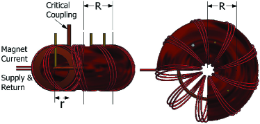
Figure 1: Lateral (left) and top (right) views of the CAPPuccino submarine. Note that it is a cut-away view to show details of the system.

We are now referring to the axion dark matter searches with toroidal geometry at our center as ACTION for “Axion haloscopes at CAPP with ToroIdal resONators” and the ACTION in this proceedings is the “simplified ACTION”. In this proceedings, we mainly show the first axion haloscope search from the simplified ACTION experiment and also discuss the prospects for larger scale ACTION experiments [2].

2 Simplified ACTION

The simplified ACTION experiment constitutes a tunable copper toroidal cavity, toroidal coils which provide a static magnetic field, and a typical heterodyne receiver chain. The experiment was conducted at room temperature. A torus is defined by $x=(R+r\cos\theta)\cos\phi$, $y=(R+r\cos\theta)\sin\phi$, and $z=r\sin\theta$, where $\phi$ and $\theta$ are angles that make a full circle of radius $R$ and $r$, respectively. As shown in Fig. 1, $R$ is the distance from the center of the torus to the center of the tube and $r$ is the radius of the tube. Our cavity tube’s $R$ and $r$ are 4 and 2 cm, respectively, and the cavity thickness is 1 cm.

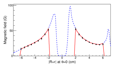
Figure 2: Magnetic field as a function of radial position $|R+r|$ at $\theta=0$. Dashed (blue) lines are obtained from the finite element method and correspond to the toroidal cavity system, and solid lines (red) correspond to the cavity tube. Dots with error bars are measurement values. The results at positive $R+r$ are along a coil, while those at negative $R+r$ are between two neighboring coils.

The frequency tuning system constitutes a copper tuning hoop whose $R$ and $r$ are 4 and 0.2 cm, respectively, and three brass posts for linking between the hoop and a piezo linear actuator that controls the movement of our frequency tuning system. The quasi-TM₀₁₀ (QTM₁) modes of the cavity are tuned by moving up and down our frequency tuning system along the axis parallel to the brass posts. Two magnetic loop couplings were employed, one for weakly coupled magnetic loop coupling and the other for critically coupled magnetic loop coupling, i.e. $\beta\simeq 1$ to maximize the axion signal power in axion haloscope searches [3].

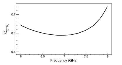
Figure 3: Form factors of the QTM₁ mode of the toroidal cavity as a function of the QTM₁ frequency.

A static magnetic field was provided by a 1.6 mm diameter copper wire ramped up to 20 A with three winding turns, as shown in Fig. 1. Figure 2 shows good agreement between measurement with a Hall probe and a simulation [4] of the magnetic field induced by the coils. The $B_{\rm avg}$ from the magnetic field map provided by the simulation turns out to be 32 G.

With the magnetic field map and the electric field map of the QTM₁ mode in the toroidal cavity, we numerically evaluated the form factor of the QTM₁ mode as a function of the QTM₁ frequency, as shown in Fig. 3, where the highest frequency appears when the frequency tuning system is located at the center of the cavity tube, such as in Fig. 1. As shown in Fig. 3, we found no significant drop-off in the form factors of the QTM₁ modes, which is attributed to the absence of the cavity endcaps in toroidal geometry.

Our receiver chain consists of a single data acquisition channel that is analogous to that adopted in ADMX [5] except for the cryogenic parts. Power from the cavity goes through a directional coupler, an isolator, an amplifier, a band-pass filter, and a mixer, and is then measured by a spectrum analyzer at the end. Cavity associates, $\nu$ (resonant frequency), and $Q_{L}$ (quality factor with $\beta\simeq 1$) are measured with a network analyzer by toggling microwave switches. The gain and noise temperature of the chain were measured to be about 35 dB and 400 K, respectively, taking into account all the attenuation in the chain, for the frequency range from 6 to 7 GHz.

The signal-to-noise ratio (SNR) in the simplified ACTION experiment is

$${\rm SNR}=\frac{P_{a,g_{a\gamma\gamma}\sim 6.5\times 10^{-8}~{}{\rm GeV}^{-1}}}{P_{n}}\sqrt{N},$$ (1)

where $P_{a,g_{a\gamma\gamma}\sim 6.5\times 10^{-8}~{}{\rm GeV}^{-1}}$ is the signal power when $g_{a\gamma\gamma}\sim 6.5\times 10^{-8}$ GeV^-1, which is approximately the limit achieved by the ALPS collaboration [6]. $P_{n}$ is the noise power equating to $k_{B}T_{n}b_{a}$, and $N$ is the number of power spectra, where $k_{B}$ is the Boltzmann constant, $T_{n}$ is the system noise temperature which is a sum of the noise temperature from the cavity ($T_{n,{\rm cavity}}$) and the receiver chain ($T_{n,{\rm chain}}$), and $b_{a}$ is the signal bandwidth. We iterated data taking as long as $\beta\simeq 1$, or equivalently, a critical coupling was made, which resulted in about 3,500 measurements. In every measurement, we collected 3,100 power spectra and averaged them to reach at least an SNR in Eq. (1) of about 8, which resulted in an SNR of 10 or higher after overlapping the power spectra at the end.

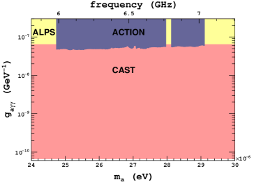
Figure 4: Excluded parameter space at the 95% C.L. by this experiment together with previous results from ALPS [6] and CAST [9]. No limits are set from 6.77 to 6.80 GHz due to with a quasi-TE mode in that frequency region and the TE mode is also confirmed by a simulation [4].

Our overall analysis basically follows the pioneer study described in Ref. [7]. With an intermediate frequency of 38 MHz, we take power spectra over a bandwidth of 3 MHz, which allows 10 power spectra to overlap in most of the cavity resonant frequencies with a discrete frequency step of 300 kHz. Power spectra are divided by the noise power estimated from the measured and calibrated system noise temperatures. The five-parameter fit also developed in Ref. [7] is then employed to eliminate the residual structure of the power spectrum. The background-subtracted power spectra are combined in order to further reduce the power fluctuation. We found no significant excess from the combined power spectrum and thus set exclusion limits of $g_{a\gamma\gamma}$ for $24.7<m_{a}<29.1$ $\mu$eV. No frequency bins in the combined power spectrum exceeded a threshold of 5.5$\sigma_{P_{n}}$, where $\sigma_{P_{n}}$ is the rms of the noise power $P_{n}$. We found $\sigma_{P_{n}}$ was underestimated due to the five-parameter fit as reported in Ref. [8] and thus corrected for it accordingly before applying the threshold of 5.5$\sigma_{P_{n}}$. Our SNR in each frequency bin in the combined power spectrum was also combined with weighting according to the Lorentzian lineshape, depending on the $Q_{L}$ at each resonant frequency of the cavity. With the tail of the assumed Maxwellian axion signal shape, the best SNR is achieved by taking about 80% of the signal and associate noise power; however, doing so inevitably degrades SNR in Eq. (1) by about 20%. Because the axion mass is unknown, we are also unable to locate the axion signal in the right frequency bin, or equivalently, the axion signal can be split into two adjacent frequency bins. On average, the signal power reduction due to the frequency binning is about 20%. The five-parameter fit also degrades the signal power by about 20%, as reported in Refs. [7, 8]. Taking into account the signal power reductions described above, our SNR for $g_{a\gamma\gamma}\sim 6.5\times 10^{-8}$ GeV^-1 is greater or equal to 10, as mentioned earlier. The 95% upper limits of the power excess in the combined power spectrum are calculated in units of $\sigma_{P_{n}}$; then, the 95% exclusion limits of $g_{a\gamma\gamma}$ are extracted using $g_{a\gamma\gamma}\sim 6.5\times 10^{-8}$ GeV^-1 and the associated SNRs we achieved in this work. Figure 4 shows the excluded parameter space at a 95% confidence level (C.L.) by the simplified ACTION experiment.

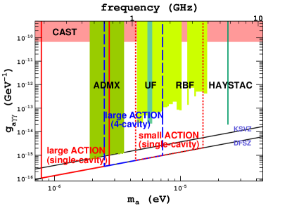
Figure 5: Expected exclusion limits by the large (solid lines with a single-cavity and dashed lines with a 4-cavity) and small (dotted lines with a single-cavity) ACTION experiments. Present exclusion limits [7, 8, 9, 10, 11, 12] are also shown.

3 Prospects for axion dark matter searches with larger scale toroidal geometry

The prospects for axion dark matter searches with two larger-scale toroidal geometries that could be sensitive to the KSVZ [13, 14] and DFSZ [15, 16] models are now discussed. A similar discussion can be found elsewhere [17]. One is called the “large ACTION”, and the other is the “small ACTION”, where the cavity volume of the former is about 9,870 L and that of the latter is about 80 L. The $B_{\rm avg}$ targets for the large and small ACTION experiments are 5 and 12 T, respectively, where the peak fields of the former and latter would be about 9 and 17 T. Hence, the large and small toroidal magnets can be realized by employing NbTi and Nb₃Sn superconducting wires, respectively. The details of the expected experimental parameters for the ACTION experiments can be found in [2] and Fig. 5 shows the exclusion limits expected from the large and small ACTION experiments.

4 Summary

In summary, we, IBS/CAPP, have reported an axion haloscope search employing toroidal geometry using the simplified ACTION experiment. The simplified ACTION experiment excludes the axion-photon coupling $g_{a\gamma\gamma}$ down to about $5\times 10^{-8}$ GeV^-1 over the axion mass range from 24.7 to 29.1 $\mu$eV at the 95% C.L. This is the first axion haloscope search utilizing toroidal geometry since the advent of the axion haloscope search by Sikivie [3]. We have also discussed the prospects for axion dark matter searches with larger scale toroidal geometry that could be sensitive to cosmologically relevant couplings over the axion mass range from 0.79 to 15.05 $\mu$eV with several configurations of tuning hoops, search modes, and multiple-cavity system.

References

- [1] B. R. Ko, “Contributed to the 12th Patras workshop on Axions, WIMPs and WISPs, Jeju Island, South Korea, June 20 to 26, 2016”; arXiv:1609.03752.
- [2] J. Choi, H. Themann, M. J. Lee, B. R. Ko, and Y. K. Semertzidis, Phys. Rev. D 96, 061102(R) (2017).
- [3] P. Sikivie, Phys. Rev. Lett. 51, 1415 (1983).
- [4] http://www.cst.com.
- [5] H. Peng et al., Nucl. Instrum. Methods Phys. Res., Sect. A 444, 569 (2000).
- [6] K. Ehret et al., Phys. Lett. B 689, 149 (2010).
- [7] C. Hagmann et al., Phys. Rev. Lett. 80, 2043 (1998); S. J. Asztalos et al., Phys. Rev. D 64, 092003 (2001).
- [8] B. M. Brubaker et al., Phys. Rev. Lett. 118, 061302 (2017).
- [9] V. Anastassopoulos et al. (CAST Collaboration), Nature Physics 13, 584-590 (2017).
- [10] S. DePanfilis et al., Phys. Rev. Lett. 59, 839 (1987); W. U. Wuensch et al., Phys. Rev. D 40, 3153 (1989).
- [11] C. Hagmann, P. Sikivie, N. S. Sullivan, and D. B. Tanner, Phys. Rev. D 42, 1297 (1990).
- [12] S. J. Asztalos et al., Astrophys. J. Lett. 571, L27 (2002); Phys. Rev. D 69, 011101(R) (2004); Phys. Rev. Lett. 104, 041301 (2010).
- [13] J. E. Kim, Phys. Rev. Lett. 43, 103 (1979).
- [14] M. A. Shifman, A. I. Vainshtein, and V. I. Zakharov, Nucl. Phys. B 166, 493 (1980).
- [15] A. R. Zhitnitskii, Sov. J. Nucl. Phys. 31, 260 (1980).
- [16] M. Dine, W. Fischler, and M. Srednicki, Phys. Lett. B 140, 199 (1981).
- [17] Oliver K. Baker et al., Phys. Rev. D 85, 035018 (2012).