Multi-epoch VLTI-PIONIER imaging of the supergiant V766 Cen

Abstract

Context. The star V766 Cen (=HR 5171A) was originally classified as a yellow hypergiant but lately found to more likely be a 27–36 $M_{\odot}$ red supergiant (RSG). Recent observations indicated a close eclipsing companion in the contact or common-envelope phase.

Aims. Here, we aim at imaging observations of V766 Cen to confirm the presence of the close companion.

Methods. We used near-infrared $H$-band aperture synthesis imaging at three epochs in 2014, 2016, and 2017, employing the PIONIER instrument at the Very Large Telescope Interferometer (VLTI).

Results. The visibility data indicate a mean Rosseland angular diameter of 4.1$\pm$0.8 mas, corresponding to a radius of 1575$\pm$400 $R_{\odot}$. The data show an extended shell (MOLsphere) of about 2.5 times the Rosseland diameter, which contributes about 30% of the $H$-band flux. The reconstructed images at the 2014 epoch show a complex elongated structure within the photospheric disk with a contrast of about 10%. The second and third epochs show qualitatively and quantitatively different structures with a single very bright and narrow feature and high contrasts of 20–30%. This feature is located toward the south-western limb of the photospheric stellar disk. We estimate an angular size of the feature of 1.7$\pm$0.3 mas, corresponding to a radius of 650$\pm$150 $R_{\odot}$, and giving a radius ratio of 0.42${}^{+0.35}_{-0.10}$ compared to the primary stellar disk.

Conclusions. We interpret the images at the 2016 and 2017 epochs as showing the close companion, or a common envelope toward the companion, in front of the primary. At the 2014 epoch, the close companion is behind the primary and not visible. Instead, the structure and contrast at the 2014 epoch are typical of a single RSG harboring giant photospheric convection cells. The companion is most likely a cool giant or supergiant star with a mass of 5${}^{+15}_{-3}$$M_{\odot}$.

1 Introduction

Red supergiants (RSGs) are cool evolved massive stars before their transition toward core-collapse supernovae (SNe). Their characterization and location in the Hertzsprung-Russell (HR) diagram are important to calibrate stellar evolutionary models of massive stars and to understand their further evolution toward SNe (e.g., Dessart et al. 2013; Groh et al. 2013, 2014). The majority of massive stars are members of binary systems with a preference for close pairs (Podsiadlowski 2010; Sana et al. 2012). Binary interactions have profound implications for the late stellar evolution of massive stars toward the different types of SNe and gamma-ray bursts (GRBs). For example, Podsiadlowski (2017) and Menon & Heger (2017) argued that the progenitor of SN1987A was likely a blue supergiant that was a member of a close binary system, where the companion dissolved completely during a common-envelope phase when the primary was a RSG.

The massive evolved star V766 Cen (=HR 5171 A) was originally classified as a yellow hypergiant (YHG, Humphreys et al. 1971; van Genderen 1992; de Jager 1998). It is known to have a wide B0 Ib companion at a separation of 9.7″. The distance to V766 Cen is well established at 3.6$\pm$0.5 kpc (Chesneau et al. 2014). Chesneau et al. (2014, in the following C14) found evidence that the primary component itself (HR 5171 A) has an eclipsing close companion, most likely in a contact or common-envelope phase. Based on VLTI-AMBER spectro-interferometry, Wittkowski et al. (2017a) reported that V766 Cen is a high-luminosity ($\log L/L_{\odot}=$ 5.8 $\pm$ 0.4) source of effective temperature 4290 $\pm$ 760 K and radius 1490 $\pm$ 540 $R_{\odot}$, located in the HR diagram close to both the Hayashi and Eddington limits. With this location and radius, it is more likely a RSG before evolving to a YHG, and consistent with a 40 $M_{\odot}$ track of current mass 27–36 $M_{\odot}$. This mass is consistent with a system mass of 39${}^{+40}_{-22}M_{\odot}$ and mass ratio $q\leq 10$ by C14.

Here, we present near-infrared $H$-band aperture synthesis images of V766 Cen with the VLTI-PIONIER instrument at multiple epochs to detect the close companion by imaging, and to investigate the surface structure of the primary.

2 Observations and data reduction

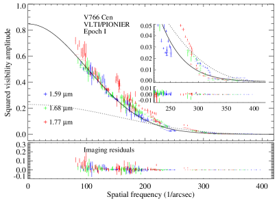
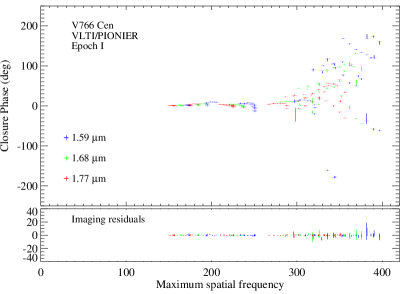
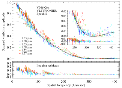
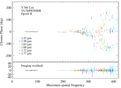
We obtained observations of V766 Cen with the PIONIER instrument (Le Bouquin et al. 2011) of the Very Large Telescope Interferometer (VLTI) and its four auxiliary telescopes (ATs). We took data at three epochs with mean Julian Day 2456719 (Feb–Mar 2016, duration 11 d), 2457528 (May–Jul 2016, 55 d), and 2457839 (Feb-Apr 2017, 64 d). The durations correspond to 0.8%, 4.2%, and 4.9%, respectively, of the estimated 1304 d period of the close companion (C14). In 2014, the data were dispersed over three spectral channels with central wavelengths 1.59 $\mu$m, 1.68 $\mu$m, 1.77 $\mu$m and channel widths of $\sim$ 0.09 $\mu$m. In 2016 and 2017, the data were dispersed over six spectral channels with central wavelengths 1.53 $\mu$m, 1.58 $\mu$m, 1.63 $\mu$m, 1.68 $\mu$m, 1.72 $\mu$m, 1.77 $\mu$m, and widths of $\sim$ 0.05 $\mu$m. Observations of V766 Cen were interleaved with observations of interferometric calibrators. The calibrators were HD 122438 (spectral type K2 III, angular uniform disk diameter $\Theta_{\mathrm{UD}}^{\mathrm{H}}=$1.23 $\pm$ 0.08 mas, used in 2014), HD 114837 (F6 V, 0.78 $\pm$ 0.06 mas, 2014), and HR 5241 (K0 III, 1.68 $\pm$ 0.11 mas, 2016 and 2017). The angular diameters are from the catalog by Lafrasse et al. (2010). Table 3 provides the log of our observations. Figure 3 shows the $uv$ coverages at each epoch, where $u$ and $v$ are the spatial coordinates of the baselines projected on sky. We reduced and calibrated the data with the pndrs package (Le Bouquin et al. 2011). Figure 4 shows all resulting visibility data of the three epochs together with a model curve as described in Sect. 3, and synthetic visibility values based on aperture synthesis imaging as described in Sect. 4.

3 Data analysis

Table 1: Fit results including the angular diameters of the photosphere ($\Theta_{\mathrm{Ross}}$) and the MOLsphere ($\Theta_{\mathrm{UD}}$), and their flux fractions $f_{\mathrm{Ross}}$ and $f_{\mathrm{UD}}$.

Epoch	$\Theta_{\mathrm{Ross}}$	$f_{\mathrm{Ross}}$	$\Theta_{\mathrm{UD}}$	$f_{\mathrm{UD}}$
	(mas)		(mas)
I	3.3	0.54	5.5	0.44
II	4.3	0.81	12.0	0.17
III	4.8	0.76	10.0	0.23
Mean	4.1$\pm$0.8	0.70$\pm$0.14	9.2$\pm$3.3	0.28$\pm$0.14

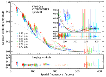
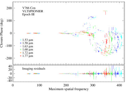
The visibility data in Fig. 4 indicate an overall spherical stellar disk. However, deviations from a continuously decreasing visibility in the first lobe and closure phases different from 0/180°at higher spatial frequencies indicate sub-structure within the stellar disk. Changes in the closure phase data among the three epochs indicate variability of the structure with time.

Previous observations (C14, Wittkowski et al. 2017a) indicated the presence of an extended molecular layer, also called MOLsphere (Tsuji 2000). We used a two-component model for the overall stellar disk, consisting of a PHOENIX model atmosphere (Hauschildt & Baron 1999) describing the stellar photosphere and a uniform disk (UD) describing the MOLsphere. We chose a PHOENIX model from the grid of Arroyo-Torres et al. (2013) with parameters close to the values from Wittkowski et al. (2017a): mass 20 $M_{\odot}$, effective temperature 3900 K, surface gravity $\log g$=-0.5, and solar metallicity. The fit was performed in the same way as in Wittkowski et al. (2017a). We treated the flux fractions $f_{\mathrm{Ross}}$ and $f_{\mathrm{UD}}$ both as free parameters to allow for an additional over-resolved background component.

Figure 4 shows our best-fit models compared to the measured data, showing that the model is successful in describing the visibility data in the first lobe. The contribution of the PHOENIX model alone is plotted to illustrate that a single-component model cannot reproduce the measured shape of the visibility function. Table 1 shows the best-fit parameters for each epoch.

Differences among the three epochs may be caused by a variability of the overall source structure, or by systematic effects such as the sparse coverage of visibility points at low spatial frequencies at epoch I. We used the averaged values and their standard deviations as final fit results as listed in Tab. 1. Our value of the Rosseland angular diameter $\Theta_{\mathrm{Ross}}$ of 4.1$\pm$0.8 mas is consistent with the estimates of $\Theta_{\mathrm{UD}}$=3.4$\pm$0.2 mas by C14 and $\Theta_{\mathrm{Ross}}$=3.9$\pm$1.3 mas by Wittkowski et al. (2017a).

4 Aperture synthesis imaging

Figure 1: Aperture synthesis images of V766 Cen at 1.58/ 1.59 $\mu$m (left), 1.68 $\mu$m (middle), and 1.77 $\mu$m (right). The three rows represent the three epochs. Contours are drawn at levels of 90%, 70%, 50%, 30%, 10%, 3% of the peak intensity. The peak intensity is normalized to unity for each image separately. The dotted circles indicate our estimated Rosseland angular diameter. The dashed circles in the lower left corners indicate the sizes of the array angular resolution $\lambda/2B_{\mathrm{max}}$.

We used the IRBis image reconstruction package by Hofmann et al. (2014) to obtain aperture synthesis images at each of our three epochs and at each of the PIONIER spectral channels. The reconstructions were performed in a similar way as for the carbon AGB star R Scl by Wittkowski et al. (2017b).

We used the best-fit models from Sect. 3 as start images. We used a flat prior, and the six available regularization functions of IRBis. We chose a pixel size of 0.3 mas, and we convolved the resulting images with a point spread function (PSF) of twice the nominal array angular resolution ($\lambda/2B_{\mathrm{max}}\sim$1.2 mas). We used a field of view of 128$\times$128 pixels, corresponding to 38.4$\times$38.4 mas, chosen to correspond to twice the best-fit size of the MOLsphere. As final images, we adopted an average of the images obtained with regularization functions 1 (compactness), 3 (smoothness), 4 (edge preservation), 5 (smoothness), and 6 (quadratic Tikhonov), which resulted in very similar images. Function 2 (maximum entropy) resulted in poorer reconstructions.

We performed a number of image reconstruction tests including the use of the reconstruction packages SQUEEZE (Baron et al. 2010) and MiRA (Thiébaut 2008), further regularization functions, and different start images. All reconstructions were very similar to those obtained with IRBis.

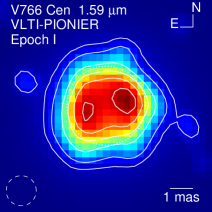
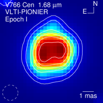
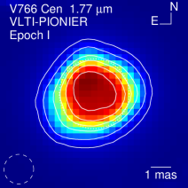
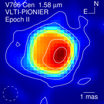
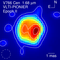
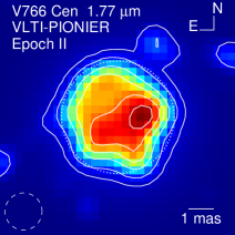
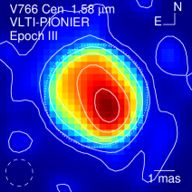
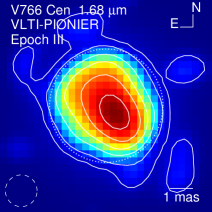
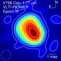
Figure 1 shows our reconstructed images for the three epochs at three spectral channels with central wavelengths 1.58/ 1.59 $\mu$m, 1.68 $\mu$m, and 1.77 $\mu$m. In Fig. 4, we over-plot the synthetic squared visibility amplitudes and closure phases based on the reconstructed images to the measured values. The residuals between both of them are also displayed. The synthetic visibility values based on the reconstructions are in good agreement with the measured values. There are discrepancies at small spatial frequencies, which increase with wavelength. This is a known systematic calibration effect of PIONIER data caused by different magnitudes or airmass between science and calibrator measurements. Values of $\chi^{2}$ for the squared visibility amplitudes range between 0.4 and 5.3, and for the closure phases between 0.22 and 2.5 for the different epochs and spectral channels. The achieved dynamic range varies between about 10 and 20.

The reconstructed images at epoch I show the stellar disk with elongated surface features approximately oriented along the East-West direction. The images at epoch II and epoch III are qualitatively different to those at epoch I. They show a dominating narrower single bright feature. The feature is located on top of the stellar disk toward its south-western limb at epoch II and oriented slightly farther toward the southern limb at epoch III. The extended molecular layer or MOLsphere as present in our model fits from Sect. 3 is not well visible in the reconstructed images because it lies just below our achieved dynamic range.

We estimated the contrast $\delta I_{\mathrm{rms}}/<I>$ (e.g., Tremblay et al. 2013) of our reconstructed images after dividing them by the best-fit model image to correct for the limb-darkening effect, and obtained values – averaged over the spectral channels and regularization functions– of 10%$\pm$4% for epoch I, 21%$\pm$6% for epoch II, and 31%$\pm$6% for epoch III. The contrasts at epochs II and III are significantly higher than those at epoch I.

We estimated the angular diameter of the feature at epochs II and III to 1.7$\pm$0.3ṁas, averaged over the epochs and spectral channels. This gives a ratio of 0.42${}^{+0.35}_{-0.10}$ compared to the Rosseland photospheric radius of the primary component.

5 Discussion and conclusions

Table 2: Estimated offsets of the companion relative to the primary

Epoch		JD	Frac.	$\Delta$ RA	$\Delta$ Dec
		d	$P_{\mathrm{orb}}$	″	″
C	(2012.18)	2455994	0	1.23	0.74
EI	(2014.17)	2456719	+0.56	/	/
EII	(2016.38)	2457528	+1.18	-0.66	-0.43
EIII	(2017.23)	2457839	+1.41	-0.89	-1.38

Figure 2: Left: Sketch of V766 Cen with the photosphere, MOLsphere, Na i shell (Wittkowski et al. 2017a), and the companion at positions from C14 (epoch C) and our epochs EII and EIII. Also shown is a plausible Keplerian orbit for a fixed period of 1304 d and semi-major axis of 3 mas. The circles indicate the positions at our epochs. Right: Illustration of an in-contact system with our radius ratio, where the companion is next to the star and we clearly see the Roche lobes (phase 0.0, top), and in front of the primary (phase 0.25, bottom). These example phases do not correspond to the observed intermediate phases in the left panel.

The images at epoch I are consistent with predictions by three-dimensional (3D) radiative hydrodynamic (RHD) simulations of RSGs, such as those shown by Chiavassa et al. (2010, Fig. 7). As an example, the contrast of this RHD $H$-band snapshot is 9%, after convolution to our spatial resolution and correction for the limb-darkening. This value is consistent with our observed value of 10%$\pm$4%. We interpret the observed surface features at epoch I by giant convection cells within the stellar photosphere.

The images at epochs II and III are significantly different to those at epoch I in terms of their appearance, that is the dominant narrower feature and their significantly higher contrast. While it may be possible that the morphology of the convection features has changed from epoch I to epochs II and III in this way, the significantly increased contrast by a factor of 3 is not consistent with current 3D simulations such as those mentioned above. In the following we explore a scenario in which the images at epochs II and III are dominated by the presence of the close companion (as suggested by C14) located in front of the primary and where at epoch I this companion is located behind the primary and not visible.

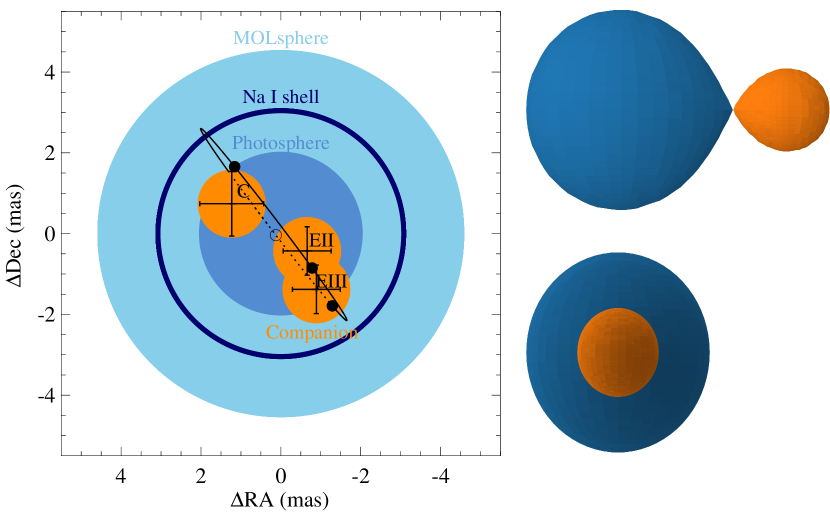
For reasons of consistency, we derived the positions at our epochs with the same fit procedure as in C14. Table 2 lists the resulting positions. The best-fit positions agree with our reconstructed images. We adopt errors of the positions of half the array angular resolution, that is 0.9 mas for the 2012 AMBER data and 0.6 mas for the 2016 and 2017 PIONIER data. Figure 2 (left) shows a sketch of V766 Cen with the photospheric disk, the MOLsphere, the Na i shell (Wittkowski et al. 2017a), and these companion positions including that of C14.

C14 analyzed available $V$ band light curve data and available radial velocity data. They could not find conclusive orbital parameters of the system, meaning that we are not able to compare our positions to a given orbit. However, they were able to constrain the orbital period to 1304$\pm$6 d based on the light curve and radial velocity data. In order to test whether our companion positions are consistent with this orbital period and thus with the light curve and radial velocity data, we explored Keplerian orbits of V766 Cen and its close companion using the fixed period of 1304 d. With the limitations of the available data, we were not able to derive any conclusive determination of the orbital parameters. However, we found an indication that semi-major axes between 2 and 5 mas with eccentricities as large as 0.5 may produce plausible orbits that are consistent with our observed angular sizes, our companion positions, and with the orbital period by C14. For illustration, Fig. 2 (left) includes an example of a plausible NE-SW orbit with a semi-major axis of 3 mas. This example orbit has a total mass of 108 $M_{\odot}$, which is above the estimates by C14 and Wittkowski et al. (2017a). The mass is sensitive to the semi-major axis and goes down to 32 $M_{\odot}$ at a semi-major axis of 2 mas. This may point to smaller angular radii of the components and a smaller semi-major axis within our error ranges. Nevertheless, this example illustrates that indeed our positions are consistent with that of C14 and with their orbital period based on the light curve and radial velocity data.

In conclusion, we interpret our images in the most likely scenario of the close eclipsing companion that is located behind the stellar disk at epoch I and in front of the stellar disk at epochs II and III. The lower contrast surface features at epoch I as well as the residual features at epochs II and III are caused by giant convection cells on the surface of the primary.

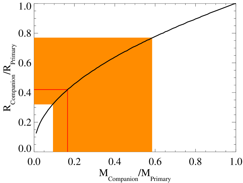
Assuming that the system is in contact or is in the common envelope phase, that is, both stars are filling their Roche lobes, we can derive the mass ratio of the components directly from the radius ratio by solving the Roche potential (Fig. 5). For a system in contact, we found that our radius ratio $R_{\mathrm{Comp}}/R_{\mathrm{Prim}}$ of 0.42${}^{+0.35}_{-0.10}$ corresponds to a mass ratio of 0.16${}^{+0.40}_{-0.07}$. This result would only be marginally affected if the system was in the common envelope phase as it mostly affects the stellar extension along the orbital plane. Figure 2 (right) illustrates an in-contact system with such a radius and mass ratio.

Our imaging observations confirm the presence of a close companion to V766 Cen observed in front of the stellar disk at two epochs. With an angular diameter of 1.7$\pm$0.3 mas, corresponding to a radius of 650$\pm$150 $R_{\odot}$ and a mass of 2–20 $M_{\odot}$, it is most likely a cool giant or supergiant. We may be witnessing a system similar to the progenitor system of SN1987 A, where a low-mass companion was dissolved during the common envelope phase when the massive progenitor was a RSG.

Appendix A Additional material

Table 3: Log of our PIONIER observations.

Date	Epoch	Configuration	# of obs.
2014-02-24	I	D0/G1/H0/I1	9
2014-03-06/-07	I	A1/G1/J3/K0	11
2016-05-07	II	A0/G1/J2/J3	6
2016-05-23/-25	II	A0/B2/C1/D0	6
2016-06-01	II	D0/G2/J3/K0	4
2016-06-27	II	A0/B2/C1/D0	2
2016-07-01	II	A0/G1/J2/J3	3
2017-02-24	III	A0/B2/C1/D0	6
2017-03-11	III	A0/B2/D0/J3	2
2017-03-15/-21	III	A0/G1/J2/J3	9
2017-04-22/-23	III	D0/G2/J3/K0	6
2017-04-24/-29	III	A0/D0/G2/J3	4

Figure 3: The $uv$ coverage obtained for our PIONIER observations of V766 Cen at epochs I (left), II (middle), and III (right).

Figure 4: Visibility results. The left panels show the squared visibility amplitudes; the inlays enlarge the low values. The right panels show the closure phases. The vertical bars indicate the symmetric error bars; different colors denote different spectral channels. The black solid lines denote our visibility model including the stellar photosphere represented by a PHOENIX model plus a larger uniform disk describing the extended molecular atmosphere. The black dashed lines indicate the contribution of the PHOENIX model alone. The synthetic values based on the reconstructed images are shown by horizontal bars. The lower small panels show the residuals between observations and reconstructed images.

Figure 5: The radius ratio $R_{\mathrm{Companion}}/R_{\mathrm{Primary}}$ as a function of the mass ratio $M_{\mathrm{Companion}}/M_{\mathrm{Primary}}$ of an in-contact system as drawn in Fig. A2 (Left) The black curve is the theoretical curve from solving the Roche potential. The red line denotes our observed radius ratio and the corresponding mass ratio, and the orange area denotes the corresponding uncertainties.

References

- Arroyo-Torres et al. (2013) Arroyo-Torres, B., Wittkowski, M., Marcaide, J. M., & Hauschildt, P. H. 2013, A&A, 554, A76
- Baron et al. (2010) Baron, F., Monnier, J. D., & Kloppenborg, B. 2010, Proc. SPIE, 7734, 77342I
- Chesneau et al. (2014) Chesneau, O., Meilland, A., Chapellier, E., et al. 2014, A&A, 563, A71 (C14)
- Chiavassa et al. (2010) Chiavassa, A., Lacour, S., Millour, F., et al. 2010, A&A, 511, A51
- de Jager (1998) de Jager, C. 1998, A&A Rev., 8, 145
- Dessart et al. (2013) Dessart, L., Hillier, D. J., Waldman, R., & Livne, E. 2013, MNRAS, 433, 1745
- Groh et al. (2014) Groh, J. H., Meynet, G., Ekström, S., & Georgy, C. 2014, A&A, 564, A30
- Groh et al. (2013) Groh, J. H., Meynet, G., Georgy, C., & Ekström, S. 2013, A&A, 558, A131
- Hauschildt & Baron (1999) Hauschildt, P. H. & Baron, E. 1999, Journal of Computational and Applied Mathematics, 109, 41
- Hofmann et al. (2014) Hofmann, K.-H., Weigelt, G., & Schertl, D. 2014, A&A, 565, A48
- Humphreys et al. (1971) Humphreys, R. M., Strecker, D. W., & Ney, E. P. 1971, ApJ, 167, L35
- Lafrasse et al. (2010) Lafrasse, S., Mella, G., Bonneau, D., et al. 2010, Proc. SPIE, 7734, 77344E
- Le Bouquin et al. (2011) Le Bouquin, J.-B., Berger, J.-P., Lazareff, B., et al. 2011, A&A, 535, A67
- Menon & Heger (2017) Menon, A. & Heger, A. 2017, ArXiv e-prints 1703.04918
- Podsiadlowski (2010) Podsiadlowski, P. 2010, New A Rev., 54, 39
- Podsiadlowski (2017) Podsiadlowski, P. 2017, ArXiv e-prints 1702.03973
- Sana et al. (2012) Sana, H., de Mink, S. E., de Koter, A., et al. 2012, Science, 337, 444
- Thiébaut (2008) Thiébaut, E. 2008, Proc. SPIE, 7013, 70131I
- Tremblay et al. (2013) Tremblay, P.-E., Ludwig, H.-G., Freytag, B., Steffen, M., & Caffau, E. 2013, A&A, 557, A7
- Tsuji (2000) Tsuji, T. 2000, ApJ, 540, L99
- van Genderen (1992) van Genderen, A. M. 1992, A&A, 257, 177
- Wittkowski et al. (2017a) Wittkowski, M., Arroyo-Torres, B., Marcaide, J. M., et al. 2017a, A&A, 597, A9
- Wittkowski et al. (2017b) Wittkowski, M., Hofmann, K.-H., Höfner, S., et al. 2017b, A&A, 601, A3
Acknowledgements.
This research has made use of the SIMBAD database, operated at CDS, France, and of NASA’s Astrophysics Data System. AA acknowledges support from the Spanish MINECO through grant AYA2015-63939-CO2-1-P, cofunded with FEDER funds.Appendix A Additional material