Deep convolutional neural networks for estimating porous material parameters with ultrasound tomography

Abstract

We study the feasibility of data based machine learning applied to ultrasound tomography to estimate water-saturated porous material parameters. In this work, the data to train the neural networks is simulated by solving wave propagation in coupled poroviscoelastic-viscoelastic-acoustic media. As the forward model, we consider a high-order discontinuous Galerkin method while deep convolutional neural networks are used to solve the parameter estimation problem. In the numerical experiment, we estimate the material porosity and tortuosity while the remaining parameters which are of less interest are successfully marginalized in the neural networks-based inversion. Computational examples confirms the feasibility and accuracy of this approach.

1 INTRODUCTION

Measuring the porous properties of a medium is a demanding task. Different parameters are often measured by different application-specific methods, e.g., the porosity of rock is measured by weighing water-saturated samples and comparing their weight with dried samples. The flow resistivity of the damping materials can be computed from the pressure drop caused to the gas flowing through the material. In medical ultrasound studies, the porosity of the bone is determined indirectly by measuring the ultrasound attenuation as the wave passes through the bone.

For the porous material characterization, information carried by waves provides a potential way to estimate the corresponding material parameters. Ultrasound tomography (UST) is one technique that can be used for material characterization purposes. In this technique, an array of sensors is placed around the target. Typically, one of the sensors is acting as a source while others are receiving the data. By changing the sensor that acts as a source, a comprehensive set of wave data can be recorded which can be used to infer the material properties. For further details on the UST, we refer to [1] and references therein.

The theory of wave propagation in porous media was rigorously formulated in 1950’s and 1960’s by Biot [2, 3, 4, 5]. The model was first used to study the porous properties of bedrock in oil exploration. Since then, the model has been applied and further developed in a number of different fields [6, 7, 8, 9]. The challenge of Biot’s model is its computational complexity. The model produces several different types of waveforms, i.e., the fast and slow pressure waves and the shear wave, the computational simulation of which is a demanding task even for modern supercomputers. Computational challenges further increase when attempting to solve inverse problems, as the forward model has to be evaluated several times.

In this work, we consider a process for the parameter estimation, comprising two sub-tasks: 1) Forward model: the simulation of the wave fields for given parameter values and 2) Inverse problem: estimation of the parameters from the measurements of wave fields. The inverse problem is solved using deep convolutional neural networks that provide a framework to solve the inverse problems: we can train a neural network as a model from wave fields to the parameters. During last decades, neural networks have been applied in various research areas such as image recognition [10, 11], cancer diagnosis [12, 13], forest inventory [14, 15], and groundwater resources [16, 17]. Deep convolutional neural networks (CNN) are a special type of deep neural networks [18, 19, 11] that employ convolutions instead of matrix multiplications (e.g. to reduce the number of unknowns). In this study, we employ deep convolutional neural networks to two-dimensional ultrasound data.

The structure of the rest of the paper is as follows. First, in Section 2, we formulate the poroviscoelastic and viscoelastic models and describe the discontinuous Galerkin method. Then, in Section 3, we describe the neural networks technique for the prediction of material parameters. Numerical experiments are presented Section 4. Finally, conclusions are given in Section 5.

1.1 Model justification

The purpose of this paper is to study the feasibility of using a data based machine learning approach in UST to characterize porous material parameters. In the synthetic model setup, we have a cylindrical water tank including an elastic shell layer. Ultrasound sensors are placed inside the water tank. In the model, we place a cylindrically shaped porous material sample in water and estimate its porosity and tortuosity from the corresponding ultrasound measurements by a convolutional neural network. Figure 1 shows a schematic drawing of a UST setup studied in this work.

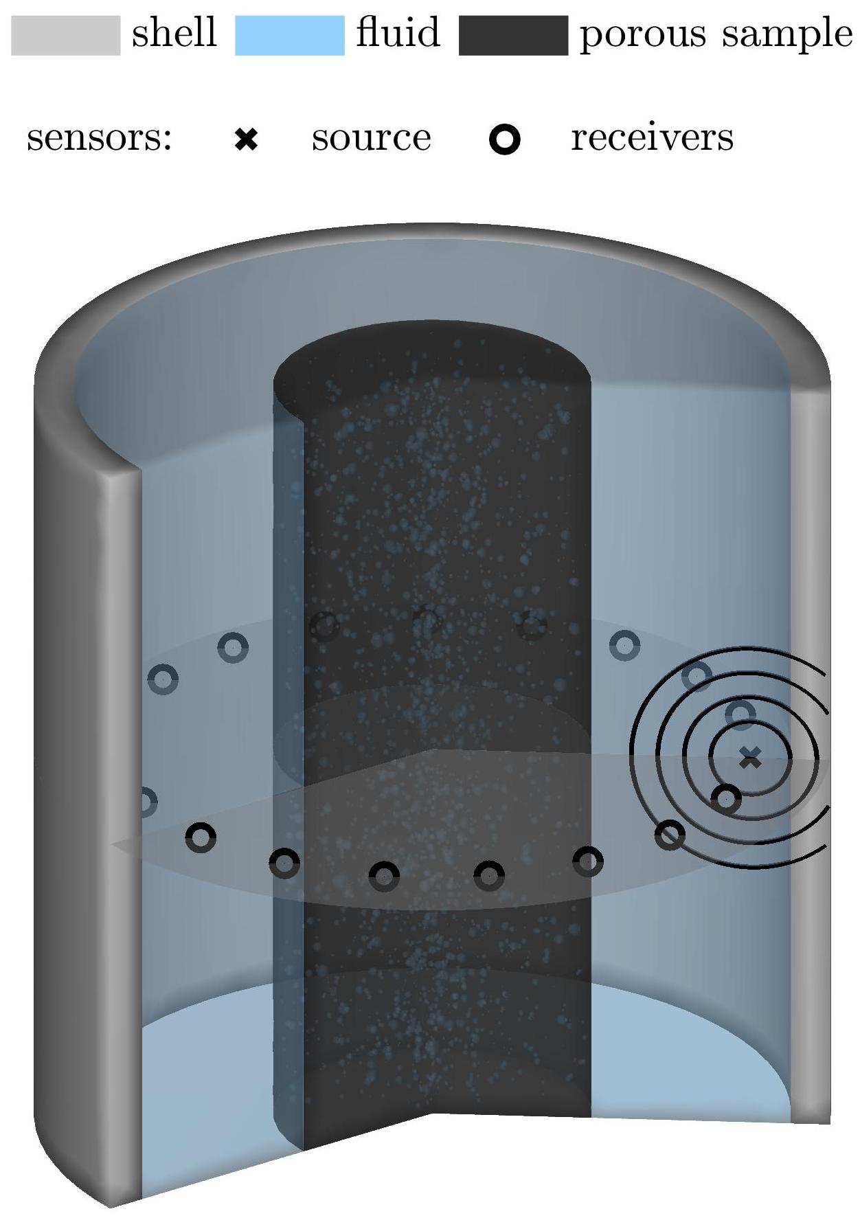
Figure 1: Schematic idea of the ultrasound tomography used to estimate porous material parameters. Acoustic wave generated by the source interact with the porous material which can be further seen on the data recovered by the receivers.

The proposed model has a wide range of potential applications. Cylindrically shaped core samples can be taken of bedrock or manmade materials, such as ceramics or concrete to investigate their properties. In addition, from the medical point of view, core samples can be taken, for example, of cartilage or bones for diagnosing purposes. Depending on the application, the model geometry and sample size together with sensor setup needs to be scaled.

2 WAVE PROPAGATION MODEL

In this paper, we consider wave propagation in isotropic coupled poroviscoelastic-viscoelastic-acoustic media. In the following Sections 2.1 and 2.2, we follow [20, 21, 22, 23] and formulate the poroviscoelastic and viscoelastic wave models. Discontinuous Galerkin method is discussed in Section 2.3.

2.1 Biot’s poroelastic wave equation

We use the theory of wave propagation in poroelastic media developed by Biot in [2, 3, 4, 5]. We express Biot equations in terms of solid displacement $\mathbf{u}_{\rm s}$ and the relative displacement of fluid $\mathbf{w}=\phi(\mathbf{u}_{\rm f}-\mathbf{u}_{\rm s})$, where $\phi$ is the porosity and $\mathbf{u}_{\rm f}$ is the fluid displacement. In the following, $\rho_{\mathrm{s}}$ and $\rho_{\mathrm{f}}$ denote the solid and fluid densities, respectively. We have

$$\rho_{\mathrm{a}}\frac{\partial^{2}\mathbf{u}_{\rm s}}{\partial t^{2}}+\rho_{\mathrm{f}}\frac{\partial^{2}\mathbf{w}}{\partial t^{2}} =\nabla\cdot{\mathbf{T}},$$ (1)

$$\rho_{\mathrm{f}}\frac{\partial^{2}\mathbf{u}_{\rm s}}{\partial t^{2}}+\frac{\rho_{\mathrm{f}}\tau}{\phi}\frac{\partial^{2}\mathbf{w}}{\partial t^{2}}+\frac{\eta}{k}\frac{\partial\mathbf{w}}{\partial t} =\nabla\cdot\mathbf{T}_{\rm f},$$ (2)

where $\rho_{\mathrm{a}}=(1-\phi)\rho_{\mathrm{s}}+\phi\rho_{\mathrm{f}}$ is the average density, $\mathbf{T}$ is the total stress tensor, and $\mathbf{T}_{\rm f}$ is the fluid stress tensor. In Eq. (2) $\tau$ is the tortuosity, $\eta$ is the fluid viscosity, and $k$ is the permeability.

The third term in (2) is a valid model at low frequencies, when the flow regime is laminar (Poiseuille flow). At high frequencies, inertial forces may dominate the flow regime. In this case, the attenuation model may be described in terms of viscous relaxation mechanics as discussed, for example, in references [21, 23]. In this paper, we use the model derived in the reference [23]. The level of attenuation is controlled by quality factor $Q_{0}$.

One can express the stress tensors as

$$\mathbf{T} = 2\mu_{\mathrm{fr}}{\bf E}+\left(\kappa_{\mathrm{fr}}+\alpha^{2}M-\frac{2}{3}\mu_{\mathrm{fr}}\right)\operatorname{tr}({\bf E}){\bf I}-\alpha M\zeta{\bf I},$$ (3)

$$\mathbf{T}_{\rm f} = M(\alpha\operatorname{tr}({\bf E})-\zeta){\bf I},$$ (4)

where $\mu_{\mathrm{fr}}$ is the frame shear modulus, $\mathbf{E}=\frac{1}{2}(\nabla\mathbf{u}_{\rm s}+(\nabla\mathbf{u}_{\rm s})^{\mathsf{T}})$ denote the solid strain tensor, $\kappa_{\mathrm{fr}}$ is the frame bulk modulus, $\operatorname{tr}(\cdot)$ is the trace, I is the identity matrix, and $\zeta=-\nabla\cdot\mathbf{w}$ is the variation of the fluid content. The effective stress constant $\alpha$ and modulus $M$, given in Eqs. (3) and (4), can be written as $\alpha=1-\kappa_{\mathrm{fr}}/\kappa_{\mathrm{s}}$, where $\kappa_{\mathrm{s}}$ is the solid bulk modulus, and $M=\kappa_{\mathrm{s}}/\left(\alpha-\phi(1-\kappa_{\mathrm{s}}/\kappa_{\mathrm{f}})\right)$, where $\kappa_{\mathrm{f}}$ is the fluid bulk modulus.

2.2 Viscoelastic wave equation

The following discussion on the elastic wave equation with viscoelastic effects follows Carcione’s book [20], in which a detailed discussion can be found. Expressed as a second order system, the elastic wave equation can be written in the following form

$$\rho_{\mathrm{e}}\frac{\partial^{2}\mathbf{u}_{\rm e}}{\partial t^{2}}=\nabla\cdot\mathbf{S}+{\bf s},$$ (5)

where $\rho_{\mathrm{e}}$ is the density, $\mathbf{u}_{\rm e}$ the elastic displacement, $\mathbf{S}$ is a stress tensor, and ${\bf s}$ is a volume source. In the two-dimensional viscoelastic (isotropic) case considered here, components of the solid stress tensor $\mathbf{S}$ may be written as [20]

$$\sigma_{11} = (\lambda_{\mathrm{e}}+2\mu_{\mathrm{e}})\epsilon_{11}+\lambda_{\mathrm{e}}\epsilon_{22}+(\lambda_{\mathrm{e}}+\mu_{\mathrm{e}})\sum_{\ell=1}^{L_{e}}\nu_{1}^{(\ell)}+2\mu_{\mathrm{e}}\sum_{\ell=1}^{L_{e}}\nu_{11}^{(\ell)},$$ (6)

$$\sigma_{22} = (\lambda_{\mathrm{e}}+2\mu_{\mathrm{e}})\epsilon_{22}+\lambda_{\mathrm{e}}\epsilon_{11}+(\lambda_{\mathrm{e}}+\mu_{\mathrm{e}})\sum_{\ell=1}^{L_{e}}\nu_{1}^{(\ell)}-2\mu_{\mathrm{e}}\sum_{\ell=1}^{L_{e}}\nu_{11}^{(\ell)},$$ (7)

$$\sigma_{12} = 2\mu_{\mathrm{e}}\epsilon_{12}+2\mu_{\mathrm{e}}\sum_{\ell=1}^{L_{e}}\nu_{12}^{(\ell)},$$ (8)

where $\mu_{\mathrm{e}}$ and $\lambda_{\mathrm{e}}$ are the unrelaxed Lamé coefficients, $\epsilon_{11},\epsilon_{22},$ and $\epsilon_{12}$ are the strain components, and $L_{e}$ is the number of relaxation terms. The memory variables $\nu_{1}^{(\ell)}$, $\nu_{11}^{(\ell)}$, and $\nu_{12}^{(\ell)}$ satisfy

$$\frac{\partial\nu_{1}^{(\ell)}}{\partial t} = -\frac{\nu_{1}^{(\ell)}}{\tau_{\sigma\ell}^{(1)}}+\phi_{1\ell}(0)(\epsilon_{11}+\epsilon_{22}),$$ (9)

$$\frac{\partial\nu_{11}^{(\ell)}}{\partial t} = -\frac{\nu_{11}^{(\ell)}}{\tau_{\sigma\ell}^{(2)}}+\frac{\phi_{2\ell}(0)(\epsilon_{11}-\epsilon_{22})}{2},\quad\ell=1,\ldots,L_{e},$$ (10)

$$\frac{\partial\nu_{12}^{(\ell)}}{\partial t} = -\frac{\nu_{12}^{(\ell)}}{\tau_{\sigma\ell}^{(2)}}+\phi_{2\ell}(0)\epsilon_{12},$$ (11)

where

$$\phi_{k\ell}(t)=\frac{1}{\tau_{\sigma\ell}^{(k)}}\left(1-\frac{\tau_{\epsilon\ell}^{(k)}}{\tau_{\sigma\ell}^{(k)}}\right)\left(\sum_{\ell=1}^{n}\frac{\tau_{\epsilon\ell}^{(k)}}{\tau_{\sigma\ell}^{(k)}}\right)^{-1}\exp\left(-t/\tau_{\sigma l}^{(k)}\right),\quad k=1,2.$$ (12)

In Eq. (12), $\tau_{\epsilon\ell}^{(k)}$ and $\tau_{\sigma\ell}^{(k)}$ are relaxation times corresponding to dilatational $(k=1)$ and shear $(k=2)$ attenuation mechanisms.

Acoustic wave equation can be obtained from the system by setting the Lamé coefficient $\mu_{\mathrm{e}}$ to zero.

2.3 Discontinuous Galerkin method

Wave propagation in coupled poroviscoelastic-viscoelastic-acoustic media can be solved using the discontinuous Galerkin (DG) method (see e.g. [24, 25, 22, 26, 23]), which is a well-known numerical approach to numerically solve differential equations. The DG method has properties that makes it well-suited for wave simulations, e.g., the method can be effectively parallelized and it can handle complex geometries and, due to its discontinuous nature, large discontinuities in the material parameters. These are all properties that are essential features for the method to be used in complex wave problems. Our formulation follows [27], where a detailed account of the DG method can be found.

3 ESTIMATING MATERIAL PARAMETERS BY NEURAL NETWORKS

The aim of this paper is to estimate porous material parameters by applying artificial neural networks trained to simulated data. Compared to traditional inverse methods, neural networks has an advantage that it allows computationally efficient inferences. In other words, after the network has been learned, inferences can be carried out using the network without evaluating the forward model. Furthermore, the neural networks provide a straightforward approach to marginalize uninteresting parameters in the inference.

First we will give a brief summary to deep neural networks. For a wider representation of the topic, the reader is pointed to review article by LeCun, Bengio, and Hinton [11], Bengio [19] or to book by Buduma [28].

We consider the following supervised learning task. We have a set of input data $\{X_{\ell}\}$ with a labels $\{Y_{\ell}\}$ ($\ell=1,\ldots,N$). In our study, the input data comprises of the measured ultrasound fields considered as “images” such that rows correspond to temporal data and columns to receiver and the outputs are corresponding material parameters. The “image” should be interpreted as two dimensional data, not a traditional picture; there is no color mapping used in our algorithm. The aim is to find a function $\Theta$ between the inputs and outputs:

$$Y=\Theta(X).$$

The task is to find a suitable form for the function and learn it from the given data. Contrary to traditional machine leaning in which the features are pre-specified, deep learning has an advantage that features are learned from the data.

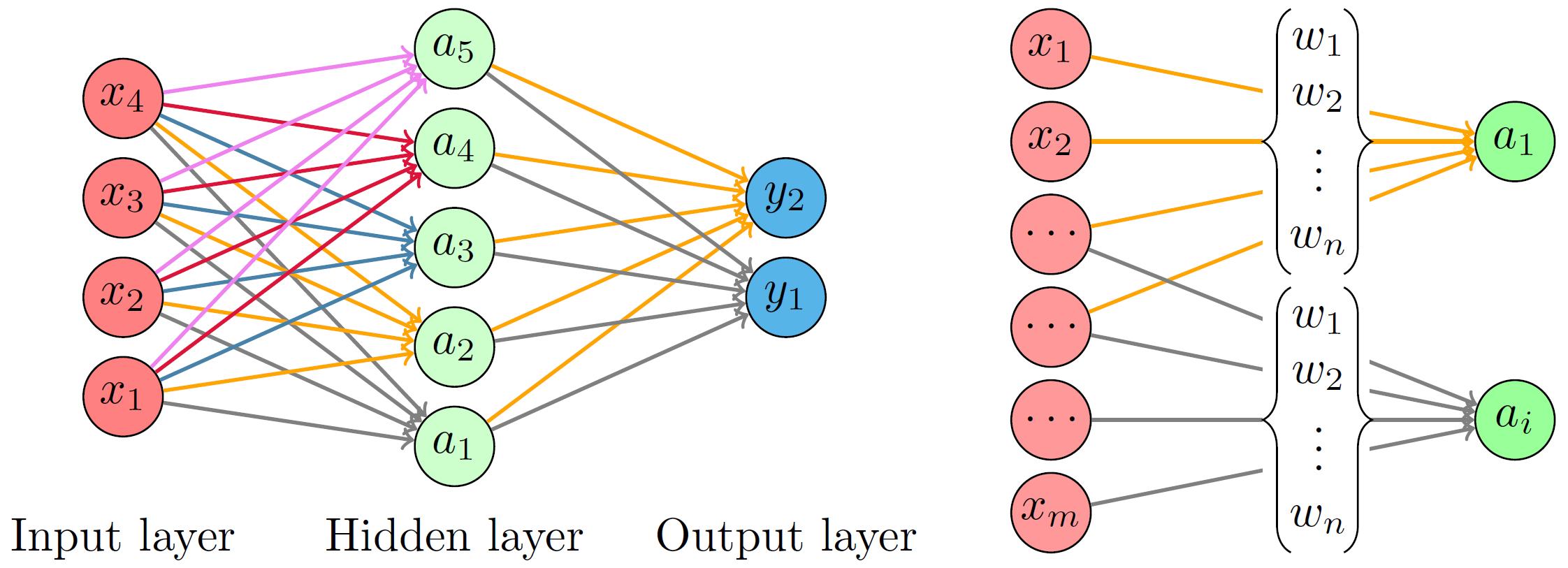
Figure 2: Left: Fully connected network with one hidden layer. Each arrow represents multiplication of the input or activation by a weight. Right: A convolutional layer. $x_{1},\ldots,x_{m}$ are the inputs to the layers and $a_{1},\ldots,a_{i}$ are the outputs of the layer. Note that the same set of the weights $w_{1},\ldots,w_{n}$ are used for all outputs.

Neural networks is a widely used class of functions in machine learning. Figure 2 (left) shows an example of a neural network with one hidden layer. Each circular node represents an artificial neuron and an arrow represents a connection between the output of one neuron to the input of the another. This network has four inputs $x_{1},\ldots,x_{4}$ (input layer), five hidden units with output activations $a_{1},\ldots,a_{5}$ (hidden layer), and two outputs $y_{1}$ and $y_{2}$ (output layer). Each neuron in the hidden layer are computational units that, for a given input $(x_{1},\ldots,x_{4})$, calculates the activations as

$$a_{j}=\sigma\left(\sum_{i=1}^{4}w^{(1)}_{ji}x_{i}+b^{(1)}_{j}\right),\quad j=1,\ldots,5,$$

where $w^{(1)}_{ji}$ is a weight assigned to the connection between the $i$th input, $b^{(1)}$ is a bias terms and $j$th activation and $\sigma$ is a non-linear function (nonlinearity). Similarly, the neurons at output layer are units for which the output is calculated as

$$y_{j}=\sigma\left(\sum_{i=1}^{5}w^{(2)}_{ji}a_{i}+b^{(2)}_{j}\right),\quad j=1,\ldots,2,$$

where $w^{(2)}_{ji}$ and $b^{(2)}_{j}$ are again weights and biases.

At the present, the most typically used nonlinearity is the Rectified Linear Unit (ReLU), $\sigma(x)=\max(0,x)$.[29] During past decades, smoother nonlinearities such as the sigmoid function $\sigma(x)=(1+\exp(-x))^{-1}$ or tanh have been used as nonlinearity, but the ReLU typically allows better performance in the training of deep neural architectures on large and complex datasets.[11] Some layers can also have different linearities than other, but here we use same $\sigma$ for notational convenience.

It is easy to see that the neural network can be presented in the matrix form as

$$A=\sigma(w^{(1)}\cdot X+b^{(1)}),\quad Y=\sigma(w^{(2)}\cdot A+b^{(2)}),$$

where $X=(x_{1},\ldots,x_{4})^{T}$, $Y=(y_{1},y_{2})^{T}$, and $A=(a_{1},\ldots,a_{5})^{T}$, $w^{(1)}$ and $w^{(2)}$ are matrices/tensors comprising of the weights $w^{(1)}_{ij}$ and $w^{(2)}_{ij}$, respectively, $b^{(1)}$ and $b^{(2)}$ are the vectors comprising of the bias variables $b^{(1)}_{i}$ and $b^{(2)}_{i}$, respectively, and the function $\sigma$ operates to the vectors element-wise. The network can be also written as a nested function $\Theta_{\theta}(X)=\sigma\left(w^{(2)}\left(\sigma(w^{(1)}\cdot X+b^{(1)})\right)+b^{(2)}\right)$ where $\theta$ represents the unknowns of the network ($\theta=(w^{(1)},b^{(1)},w^{(2)},b^{(2)})$).

Deeper networks can be constructed similarly. For example, a network with two hidden layers can be formed as $A^{(1)}=\sigma(w^{(1)}\cdot X+b^{(1)})$, $A^{(2)}=\sigma(w^{(2)}\cdot A^{(1)}+b^{(2)})$ and $Y=\sigma(w^{(3)}\cdot A^{(2)}+b^{(3)})$, or $\Theta_{\theta}(X)=\sigma\left(w^{(3)}\cdot\sigma\left(w^{(2)}\cdot\left(\sigma(w^{(1)}\cdot X+b^{(1)})\right)+b^{(2)}\right)+b^{(3)}\right)$ where $\theta=(w^{(1)},b^{(1)},w^{(2)},b^{(2)},w^{(3)},b^{(3)})$.

The neural networks described above are called fully connected: there are connections between all nodes of the network. A disadvantage of such fully connected networks is that total number of free parameters can be enormous especially when the dimensions of input data is high (e.g. high resolution pictures) and/or the network has several hidden layers. Convolutional neural networks (CNN) were introduced [30, 18] to overcome this problem. Figure 2 (right) shows an example of a 1D-convolutional layer. In a convolutional layer, the matrix multiplication is replaced with a convolution: for example, in 1D, the activations of the layer are calculated as

$$A=\sigma\left(w^{(1)}*X+B^{(1)}\right),$$

where $*$ denotes the discrete 1D-convolution and $w^{(1)}$ is a set of filter weights (a feature to be learned). In 2D, the input $X$ can be considered as an image and the convolution $w^{(1)}*X$ is two dimensional with a convolution matrix or mask $w^{(1)}$ (a filtering kernel).

In practical solution, however, only one convolution mask (per layer) is typically not enough for good performance. Therefore, each layer includes multiple masks that are applied simultaneously and the output of the convolutional layer is a bank (channels) of images. This three dimensional object forms the input of the next layer such that each input channel has own bank of filtering kernels and the convolution is effectively three dimensional.

Usually convolutional neural networks employs also pooling [31, 10] for down-sampling (to reduce dimension of activations). See for example LeCun, Bengio, and Hinton [11] or Buduma [28] for details.

The training of the neural networks is based on a set of training data $\{X_{\ell},Y_{\ell}\}$. The purpose is to find a set if weights and biases that minimize the discrepancy between the outputs $\{Y_{\ell}\}$ and the corresponding predicted values given by the neural networks $\{\Theta_{\theta}(X_{\ell})\}$. Typically, in regression problems, this is achieved by minimizing the quadratic loss function $f(\theta)$ over the simulation dataset

$$f(\theta)=f(\theta;\{X_{\ell}\},\{Y_{\ell}\})=\frac{1}{N_{nn}}\sum_{\ell=1}^{N_{nn}}{\left(\Theta_{\theta}(X_{\ell})-Y_{\ell}\right)^{2}}$$ (13)

to obtain the network parameters, weights, and biases, of the network. The optimization problem could be solved using gradient descent methods. The gradient can be calculated using back propagation which essentially is a procedure of applying the chain rule to the lost function in an iterative backward fashion [32, 28, 11]. The computations of the predictions $\Theta_{\theta}(X_{\ell})$ and its gradients is computationally expensive task in the case of large training dataset. Therefore, during the iteration, the cost and gradients are calculated for mini-batches that are randomly chosen from the training set. This procedure is called as stochastic gradient descent (SGD) [18, 28].

The validation of the network is commonly carried out using a test set, which is either split from the original data or collected separately. This test set is used to carry final evolution of the performance. This is done due to the tendency of deep networks for overfitting, which comes out as a good performance in the training set but very poor performance in test set (i.e. the network “remembers” the training samples instead of learning to generalize). Third set, the validation data set, is also traditionally used to evaluate performance during the training process.

4 NUMERICAL EXPERIMENT

In this section, we present the results obtained from testing the data driven approach to estimate porous material parameters in ultrasound tomography. In this paper, initial conditions are always assumed to be zero and we apply the free condition as a boundary condition.

In the following results, time integration is carried out using an explicit low-storage Runge-Kutta scheme [33]. For each simulation, the length of the time step $\Delta t$ is computed from

$$\Delta t=\left(\frac{h^{\ell}_{\min}}{2c^{\ell}_{\max}(N^{\ell})^{2}}\right)_{\min},\quad\ell=1,\ldots,K,$$ (14)

where $c^{\ell}_{\max}$ is the maximum wave speed, $N^{\ell}$ is the order of the polynomial basis, $h^{\ell}_{\min}$ is the smallest distance between two vertices in the element $\ell$, and $K$ is the number of elements.

4.1 Model setup

Let us first introduce the model problem. Figure 3 shows the studied two dimensional problem geometry. The propagation medium contains three subdomains: a cylindrical shaped poroelastic inclusion (black), a fluid (light gray), and a solid shell (dark gray). The computational domain is a circle with radius of 10 cm with a 1 cm thick shell layer. A circular shaped poroelastic inclusion with a radius of 4 cm is vertically shifted to 2 cm from the center of the circular domain. Shifting the target from the center avoids symmetrically positioned sensors (with respect to x-axis) to receive equal signal and therefore have more information from the target.

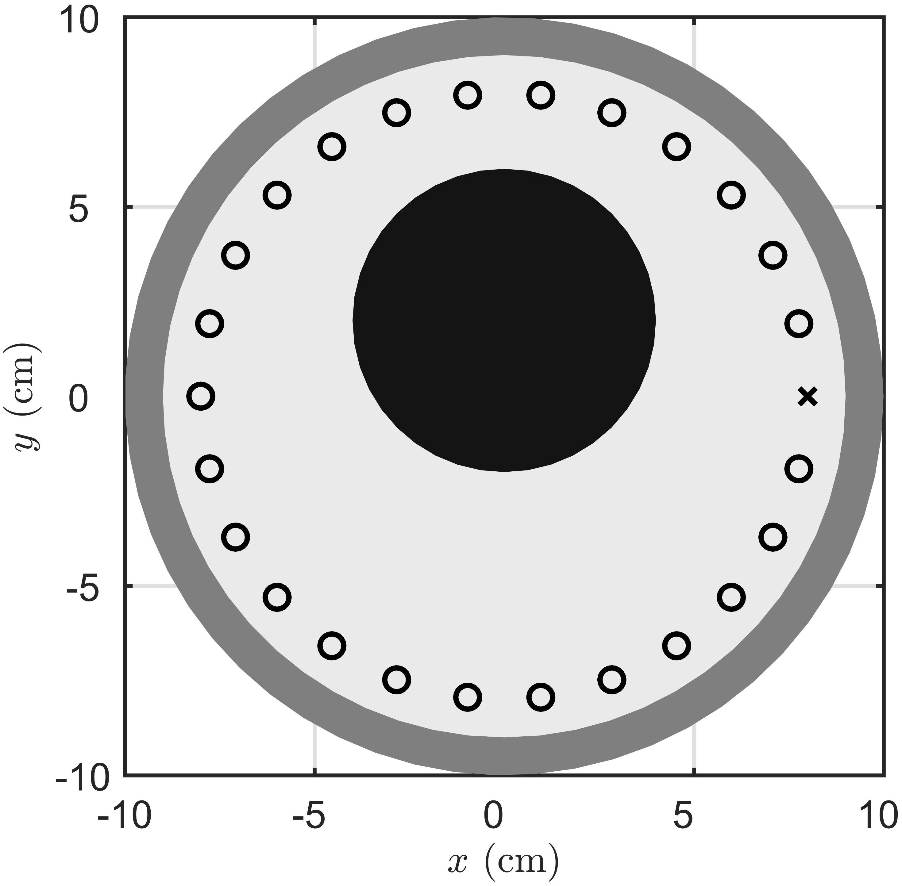
Figure 3: Figure shows the problem geometry. In the graph, the circles denote the receivers and the cross denotes the source.

A total of 26 uniformly distributed ultrasound sensors are located at a distance of 8 cm from the center of the circle. The source is introduced on the strain components $\epsilon_{11}$ and $\epsilon_{22}$ by the first derivative of a Gaussian function with frequency $f_{0}=40$ kHz, a time delay $t_{0}=1.2/f_{0}$. The sensor that is used as a source does not collect data in our simulations. Receivers collect solid velocity components $u_{\rm s}$ and $v_{\rm s}$. In the following, the simulation time is 0.4 ms. Note that recorded data is downsampled to a sampling frequency of 800 kHz on each receiver.

The inclusion is fully saturated with water. The fluid parameters are given by: the density is $\rho_{\mathrm{f}}=1020$ kg/m³, the fluid bulk modulus is $\kappa_{\mathrm{f}}=2.295$ GPa, and the viscosity is $\eta=1.0$e-3 Pa$\cdot$s. All other material parameters of the inclusion are assumed to be unknown. In this paper, we assume a relatively wide range of possible parameter combinations, see Table 1. Furthermore, the unknown parameters are assumed to be uncorrelated. The physical parameter space gives $\sim$1.5 kHz as an upper bound for Biot’s characteristic frequency

$$f_{c}=\frac{\eta\phi}{2\pi\tau\rho_{\mathrm{f}}k}$$ (15)

and hence we operate in Biot’s high-frequency regime $(f_{c}<f_{0})$ in all possible parameter combinations.

Table 1: Table lists the minimum and maximum values used for uniform distributions for each unknown physical parameter.

variable name	symbol	minimum	maximum
solid density	$\rho_{\mathrm{s}}$ (kg/m3)	1000.0	5000.0
solid bulk modulus	$\kappa_{\mathrm{s}}$ (GPa)	15.0	70.0
frame bulk modulus	$\kappa_{\mathrm{fr}}$ (GPa)	5.0	20.0
frame shear modulus	$\mu_{\mathrm{fr}}$ (GPa)	3.0	14.0
tortuosity	$\tau$	1.0	4.0
porosity	$\phi$	0.01	0.99
permeability	$k$ (m2)	1.0e-10	1.0e-7
quality factor	$Q_{0}$	20.0	150.0

For the fluid subdomain (water), we set: the density $\rho_{\mathrm{e}}=1020$ kg/m³, the first Lamé parameter $\lambda_{\mathrm{e}}=2.295$ GPa, and the second Lamé parameter $\mu_{\mathrm{e}}=0$. The elastic shell layer has the following parameters: $\rho_{e}=2000$ kg/m³, $\lambda_{e}=12.940$ GPa, and $\mu_{e}=5.78$ GPa. The relaxation times for the viscoelastic attenuation in the shell layer are given in Table 2.

Table 2: Table lists the relaxation times (two mechanisms) used with the shell layer. Relaxation times are computed using the nonlinear optimization method discussed in detail in [34].

	$\tau_{\epsilon\ell}^{(1)}$	$\tau_{\sigma\ell}^{(1)}$	$\tau_{\epsilon\ell}^{(2)}$	$\tau_{\sigma\ell}^{(2)}$
$\ell=1$	1.239e-4	1.176e-4	1.249e-4	1.165e-4
$\ell=2$	5.319e-6	5.042e-6	5.370e-6	4.999e-6

The derived wave speeds for each subdomain are given in Table 3. For the poroelastic inclusion, both the minimum and maximum wave speeds are reported. It should be noted that the reported values for the wave speeds in the inclusion correspond to the values generated by sampling the material parameters and hence they may not correspond to the global maximum and minimum values. A detailed approach for calculating wave speeds is given in [23].

Table 3: Derived wave speeds for each subdomain. For the inclusion, both the minimum/maximum values are given. For the inclusion, values are based on sampling the material parameters.

subdomain	$c_{p}^{\mathrm{I}}$ (m/s)	$c_{p}^{\mathrm{II}}$ (m/s)	$c_{s}$ (m/s)
inclusion	1900/20189	196/1983	833/11578
fluid	1500	-	-
shell	3500	-	1700

It should be noted that, depending on the application, only some of the material parameters are unknowns of interest. In this work, we focus on estimating the porosity and tortuosity of the inclusion while the solid density and bulk modulus, frame bulk and shear modulus, permeability, and quality factor are marginalized in the neural networks-based inversion algorithm, discussed in detail below.

4.2 Training, validation, and test data

For the convolutional neural networks algorithm used in this work, the recorded wave data is as expressed as images $X\in\mathbb{R}^{d},\ d=N_{t}\times N_{r}$, where $N_{t}$ denotes the number of time steps and $N_{r}$ the number of receivers. The input dimension is $d=320\times 25$, as the data $X$ can be seen as a 2D-image, comprising 25 pixels, corresponding to the receiver positions, times 320 pixels corresponding to the time evolution of the signal.

As the data on each column of the image, we use the following

$$X(:,\ell)=\frac{x_{r}^{\ell}(u_{\rm s}^{\ell}-u_{{\rm s},noi}^{\ell})+y_{r}^{\ell}(v_{\rm s}^{\ell}-v_{{\rm s},noi}^{\ell})}{\sqrt{(x_{r}^{\ell})^{2}+(y_{r}^{\ell})^{2}}},\quad\ell=1,\ldots,N_{r},$$ (16)

where $(x_{r}^{\ell},\ y_{r}^{\ell})$ are the coordinates of the $\ell$th receiver and $(u_{\rm s}^{\ell},\ v_{\rm s}^{\ell})$ are the horizontal and vertical velocity components on the $\ell$th receiver. In Eq. (16) subscript $noi$ denotes the data that is simulated without the porous inclusion. Two example images are shown in Fig. 4.

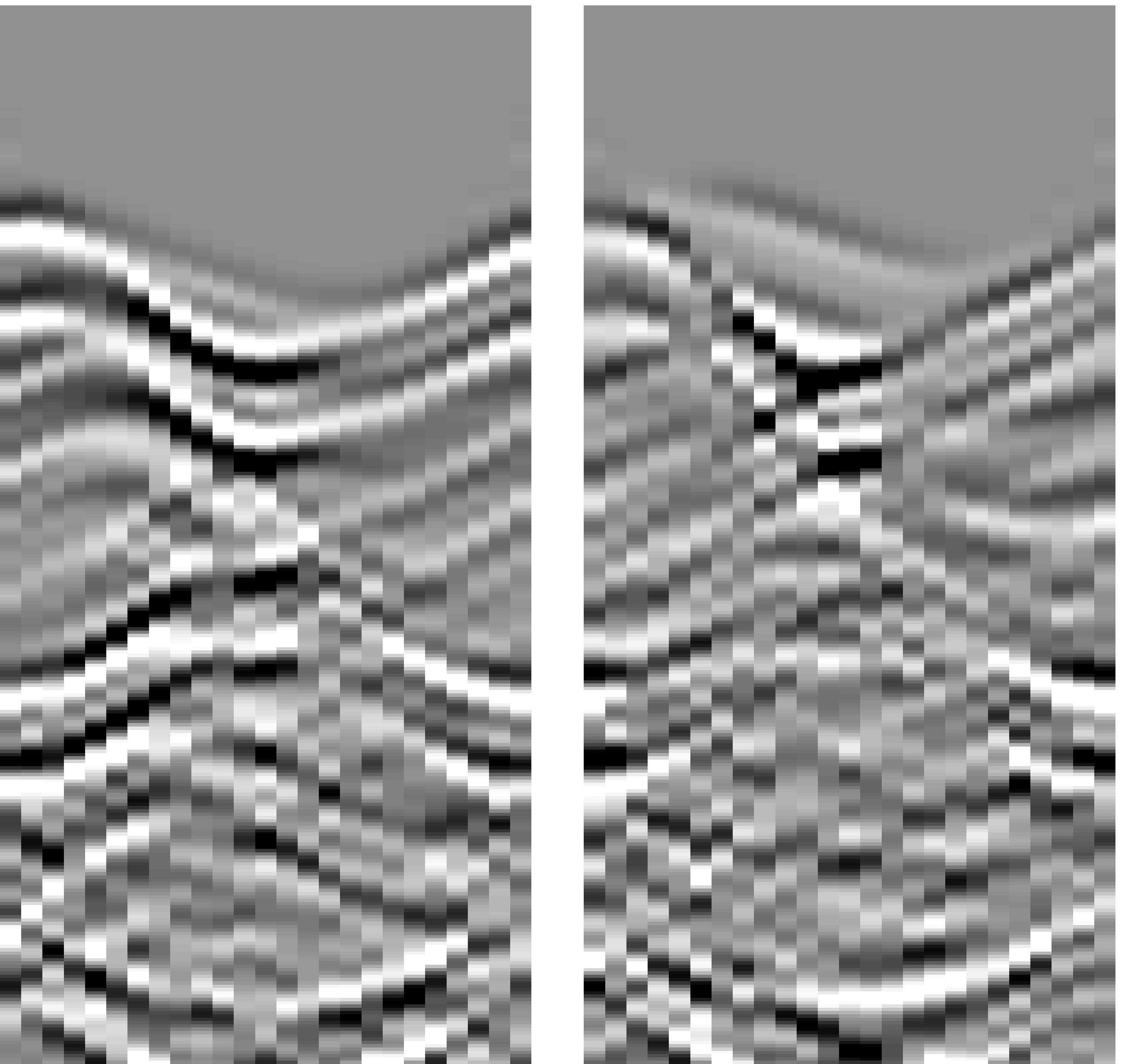
Figure 4: Example images used for training the neural networks algorithm. Note that neural networks algorithm uses the original pixel values of the image $X$ (see Eq. (16)). Time is shown on the vertical-axis and receiver index on the horizontal-axis. Images correspond to samples where the shear wave speeds $c_{s}$ is minimum (left) or maximum (right) (see Table 3).

We have generated a training data set comprising 15,000 samples using computational grids that have $\sim$3 elements per wavelength. The physical parameters for each sample are drawn from the uniform distribution (bounds given in Table 1). The order of the basis functions is selected separately for each element of the grid. The order $N_{\ell}$ of the basis function in element $\ell$ is defined by

$$N_{\ell}=\left\lceil\frac{2\pi ah^{\ell}_{\max}}{\lambda^{w}_{\ell}}+b\right\rceil,$$ (17)

where $\lambda^{w}_{\ell}=c^{\ell}_{\min}/f_{0}$ is the wavelength, $c^{\ell}_{\min}$ is the minimum wave speed, and $\lceil\cdot\rceil$ is the ceiling function. The parameters $a$ and $b$ control the local accuracy on each element. Following [35, 36], we set $(a,\ b)=(1.0294,\ 0.7857)$.

Figure 5 shows two examples of computational grids and the corresponding basis order selection on each triangle. Example grids consist of 466 elements and 256 vertices ($h_{\min}=0.81$ cm and $h_{\max}=1.95$ cm) (sample 1) and 1156 elements and 601 vertices ($h_{\min}=0.32$ cm and $h_{\max}=1.75$ cm) (sample 2).

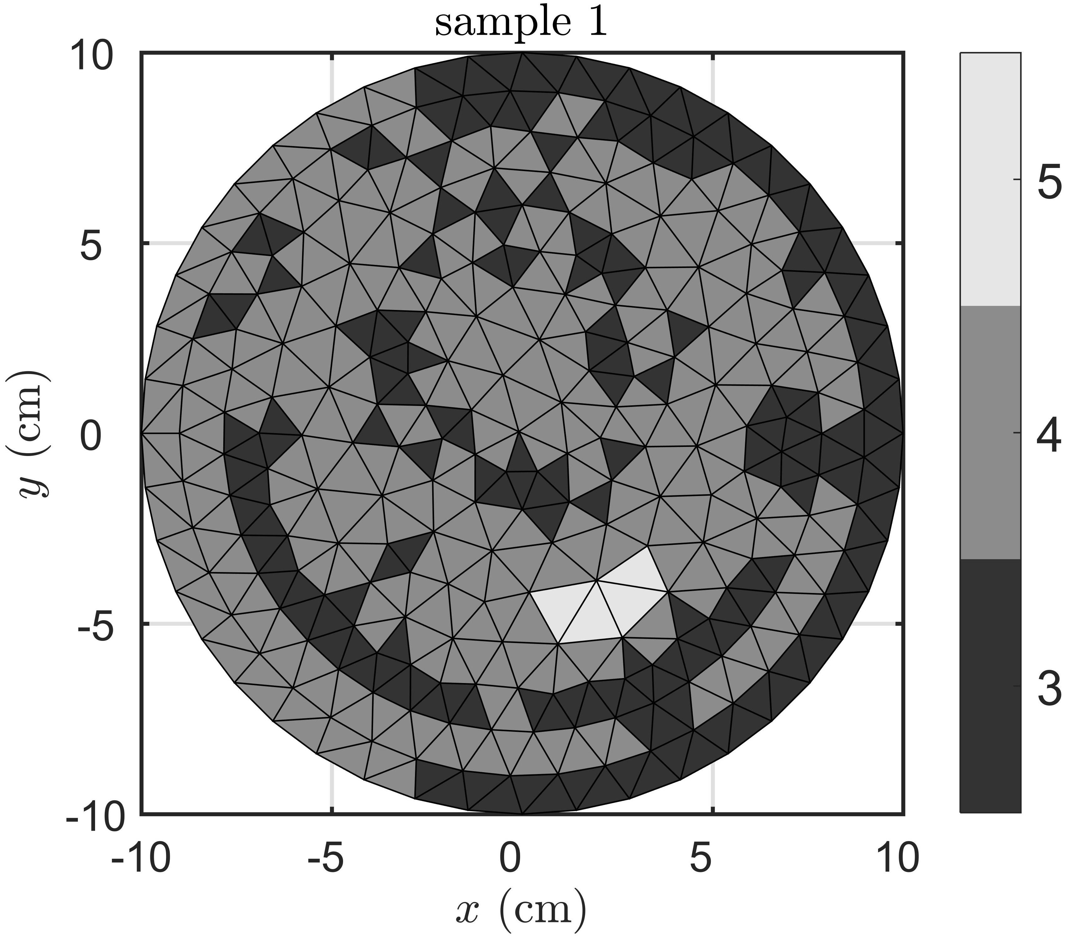
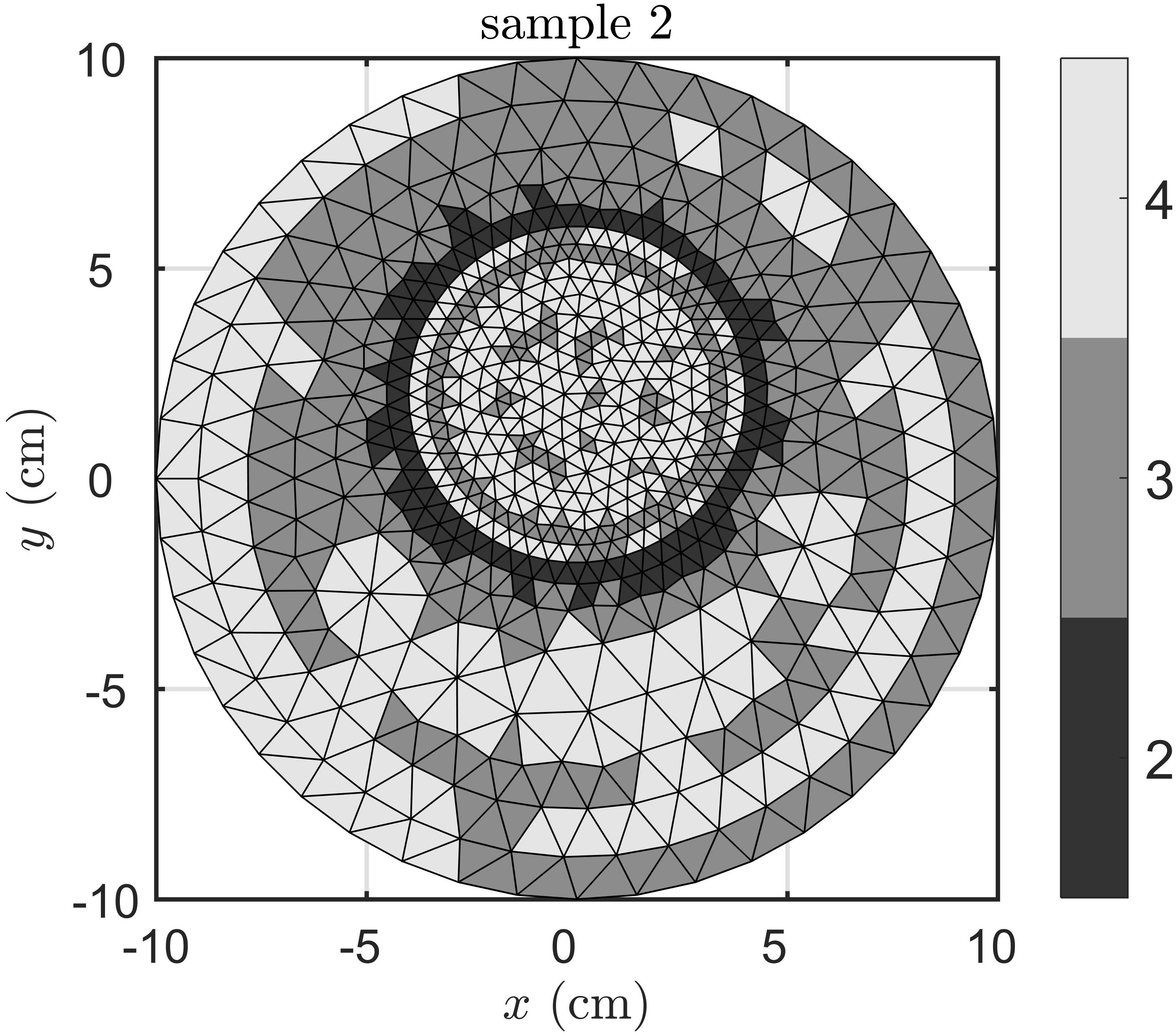
Figure 5: Figure shows two example grids used in the computations. The colorbar shows the order of the basis functions.

Figure 6 shows two snapshots of the scattered solid velocity field ($\sqrt{(u_{\rm s}-u_{{\rm s},noi})^{2}+(v_{\rm s}-v_{{\rm s},noi})^{2}}$) for two time instants. At the first time instant, the transmitted fast pressure wave and also the first reflected wave front is clearly visible. At the second time, all wave components have reflected back from the left surface of the phantom. Furthermore, more complicated wave scattering patterns can be seen inside the porous inclusion. These wave fields demonstrate how the received signals are obtained as combinations of multiple wave fronts.

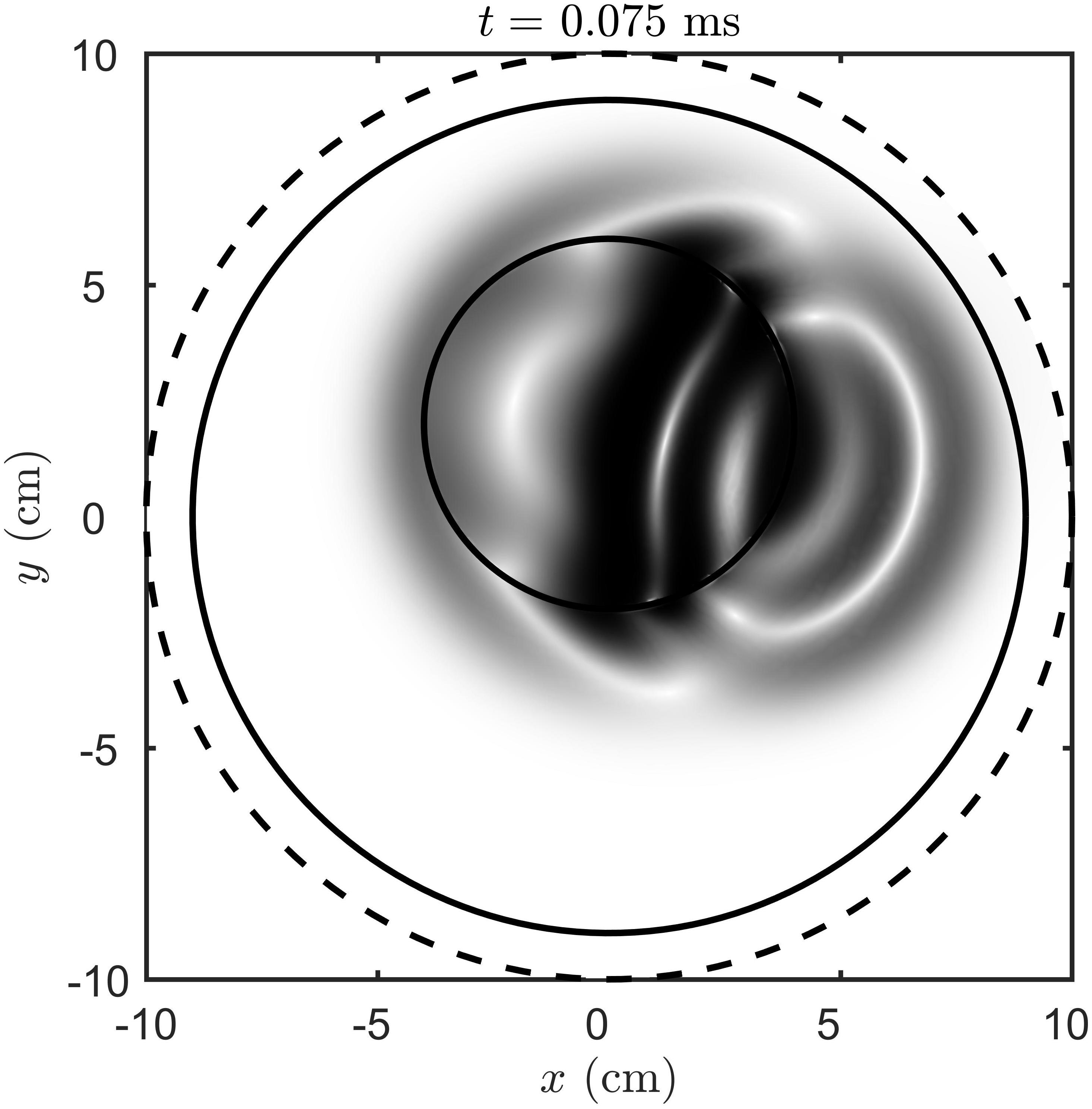
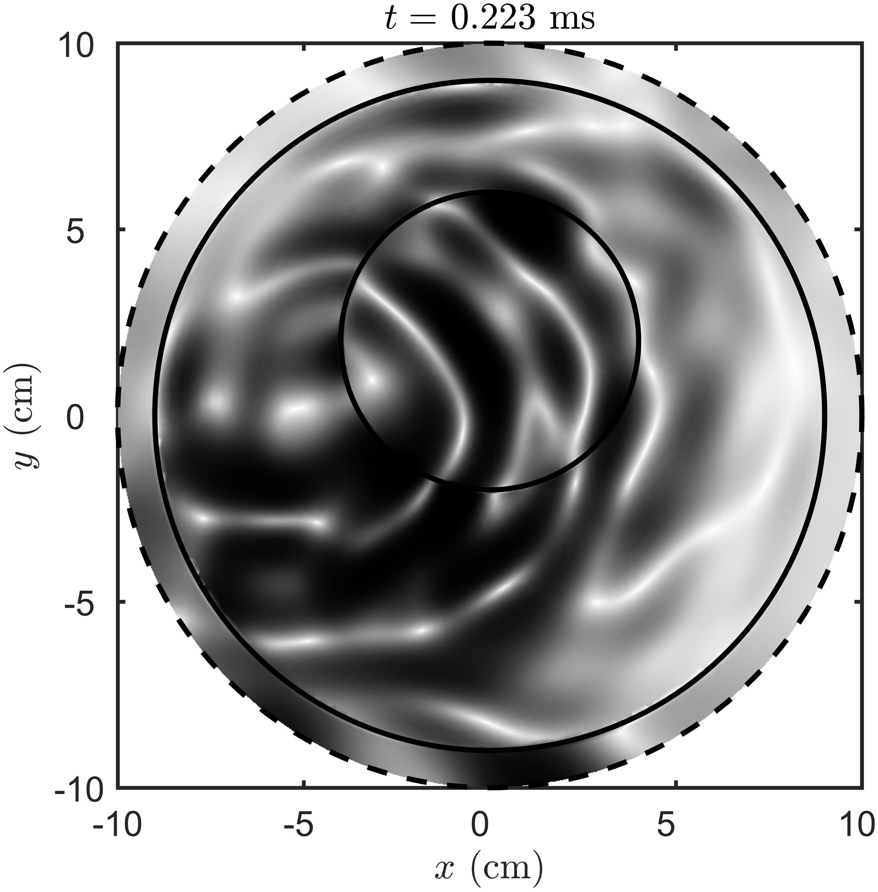
Figure 6: Wave interaction with the poroelastic material at two times. The title shows the time. In the graphs, solid black lines show the inclusion/water and water/shell interfaces while the dotted black line shows the exterior boundary.

To include observation noise in the training, each image in the simulation set is copied 5 times and each of the copies is corrupted with Gaussian noise of the form

$$X_{\ell^{\prime}}^{\textrm{noised}}=X_{\ell}+A\epsilon^{A}+B|X_{\ell}|\epsilon^{B},$$ (18)

where $\epsilon^{A}$ and $\epsilon^{B}$ are independent zero-mean identically distributed Gaussian random variables. The second term represents additive white noise and the last term represents noise relative the signal strength. To represent a wide range of different noise levels, for each sample image, the coefficients $A$ and $B$ are randomly chosen such that the standard deviations of the white noise component is between 0.03-5% (varying logarithmically), and the standard deviations of the relative component is between 0-5%. The total number of samples in the training set is $N_{nn}=5\times 15000=75000$.

Furthermore, two additional data sets were generated: a validation data set and a test set, that both comprise 3000 samples. In machine learning, the validation data set is traditionally used to evaluate performance during the training process and the test set is used for the final evaluation of the network. These data sets are generated similarly as the training set, except computational grids were required to have $\sim$4 elements per wavelength to avoid inverse crime [37]. Furthermore, for the test set, the non-uniform basis order parameters are $(a,\ b)=(1.2768,\ 1.4384)$ [35] (Eq. (17)) and the noise is added in a more systematic manner (instead of choosing $A$ and $B$ are randomly) to study the performance with different noise levels (see Results section).

4.3 Convolutional neural networks architecture

The neural network architecture is shown in Table 4 and Fig. 7. The CNN architecture is similar to ones used for image classification, for example, Alexnet [10], with some exceptions. In our problem, the input data can be considered as one channel images instead of color images with three channels (i.e. we do not apply any color mapping). Our network also lacks the softmax layer, which is used as an outmost layer to provide the classification. Instead, the outmost two layers are simply fully connected layers. In addition, our network also has smaller number of convolutional and fully connected layers with and smaller dimensions in filter banks, which leads to significantly smaller number of unknowns. We, however, wish to note that purpose aim was not to find the most optimal network architecture. For example, there can be other architectures that can provide similar performance with even smaller number of the unknowns. Furthermore, similar performance can also be achieved with fully connected networks with $\sim$3 layers, but at the expense of significantly larger number of unknowns.

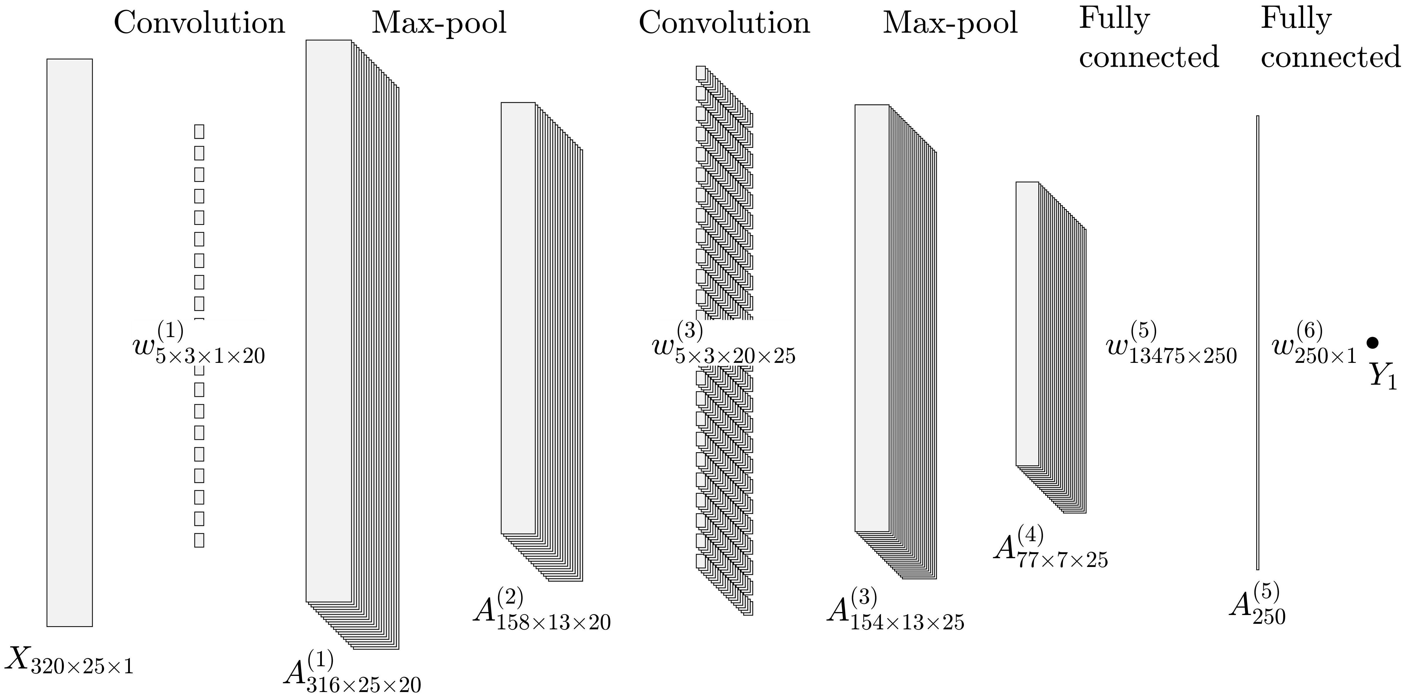
Figure 7: A flow diagram of the network used in the study. Flow is from left to right (connecting arrows are not shown for graphical clarity). The sizes of the boxes scale with the memory size of the elements. The size/structure of the neurons and weights are also displayed in the subscript of $A^{(i)}$ and $w^{(i)}$ for each layer $i$. The matrices of the weights of the full connected layers $w^{(5)}$ and $w^{(6)}$ are not drawn for graphical clarity.

The loss function is chosen to be quadratic (Eq. (13)). The implementation is carried out using Tensorflow, which is a Python toolbox for machine learning. The optimization was carried out with the Adam optimizer [38]. The batch size for the stochastic optimization is chosen to be 50 samples.

Table 4: The convolutional neural network architecture used in this work. The convolutional layers uses periodic convolution (padding) in the receiver position-direction and no padding in the temporal direction. The total number of unknowns in the network is 3.38M.

Layer k	Type and non-linearity	input size	output size
	Input	$320\times 25$	$320\times 25\times 1$
1	Convolution layer ($5\times 3\times 1$ filter, 20 filters)	$320\times 25\times 1$	$316\times 25\times 20$
	+ Layer normalization + ReLU
	+ Max-pooling ($2\times 2$)	$316\times 25\times 20$	$158\times 13\times 20$
2	Convolution layer ($5\times 3\times 20$ filter, 25 filters)	$158\times 13\times 20$	$154\times 13\times 25$
	+ Layer normalization + ReLU
	+ Max-pooling ($2\times 2$)	$154\times 13\times 25$	$77\times 7\times 25$
3	Vectorization	$77\times 7\times 25$	13475
	Fully connected layer	13475
	+ Layer normalization + ReLU		250
4	Fully connected layer	250	1
	Output		1

4.4 Results

Figure 8 shows the loss of the training and validation data. The loss is shown for the two unknown parameters of interest, e.g., porosity and tortuosity. In both cases, we observe that the network has practically reached its generalization capability at least after 2000 full training cycles. The accuracy of the network is affected by the marginalization over all other parameters. In principle, the effect of the other parameters could compensate the changes that using, for example, a different porosity would cause, leaving the waveform of the measurement intact.

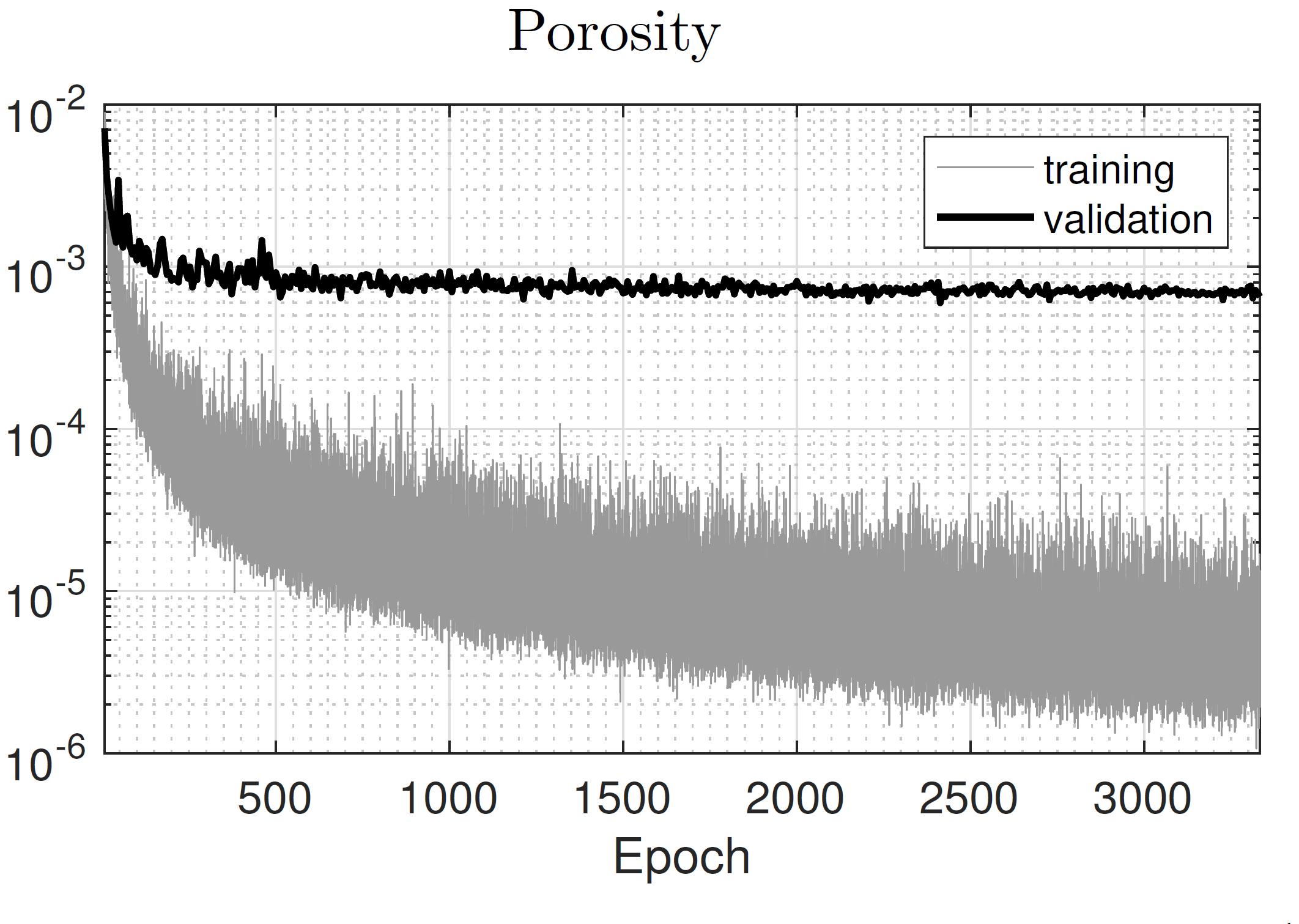
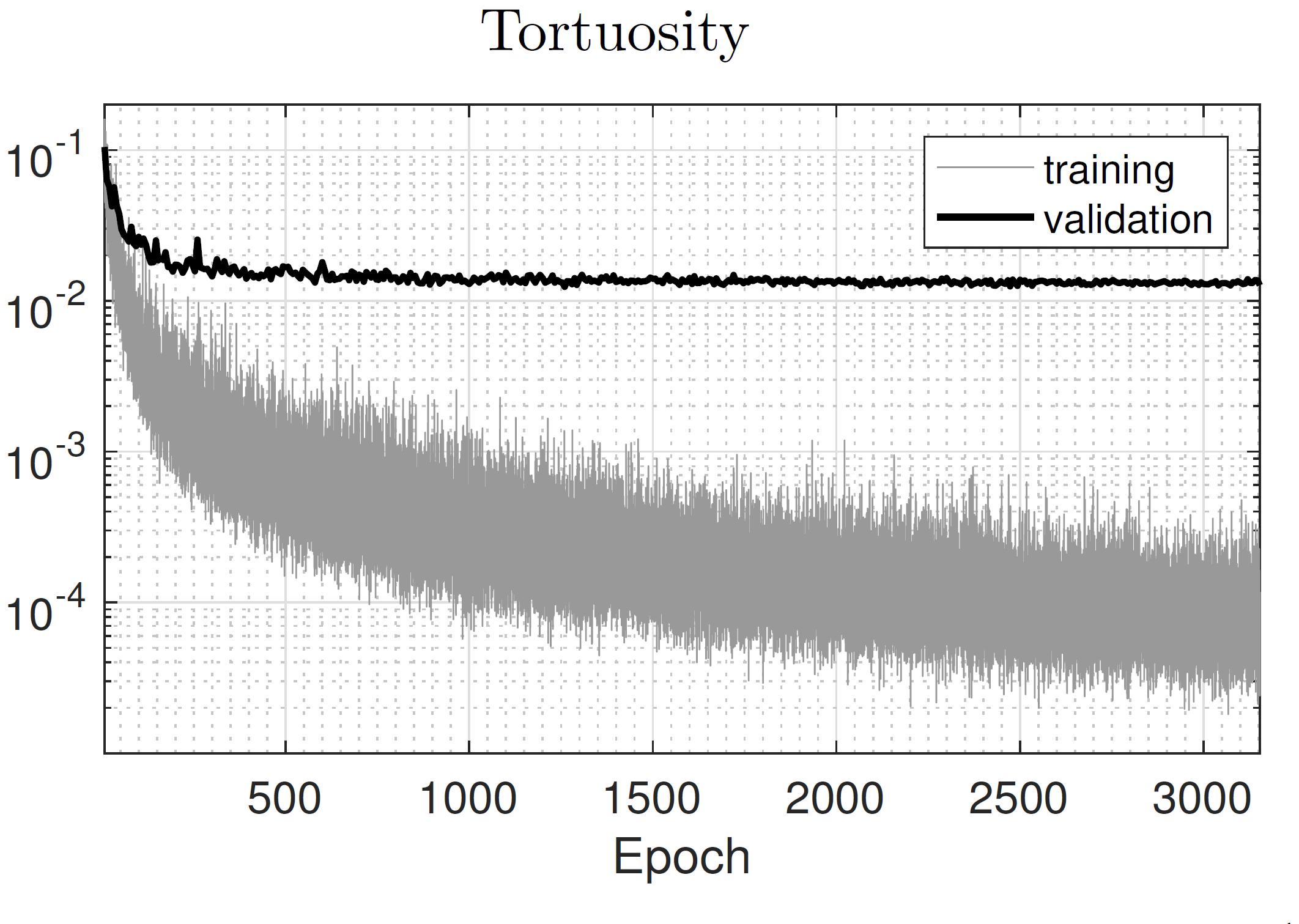
Figure 8: Training and validation loss for porosity (left) and tortuosity (right) as function of number of epochs (full training cycles in stochastic optimization).

We have applied the trained network to predict porosity and tortuosity from images of the test that are corrupted with the white noise component with low noise level (Fig. 9), moderate noise level (Fig. 10), and high noise level (Fig. 11). The figures also include error histograms. Table 5 shows statistics of the prediction error for different noise levels. Figure 12 shows the maximum absolute error and the root-mean-square error (the square root of Eq. (13)) as a function of the noise level in white noise component. The predictions are slightly positively biased with smaller noise levels, but positive bias is diminished with higher noise levels. Such a behavior might be due to the discretization error in forward models (the simulation of training and testing data were carried out using different levels of discretizations) which may dominate with lower observation noise levels but becomes negligible with higher noise levels. On the contrary, with high levels of noise, the predictions are negatively biased especially for larger values of porosity and tortuosity.

We have also studied the effect of the relative noise (the third term in Eq. (18)) to the results. Figure 13 shows the maximum absolute error and the root-mean-square error as a function of the noise level in the relative component. As we can see, the predictions are almost unaffected by the relative error even with significantly high noise levels ($\sim$5-10%).

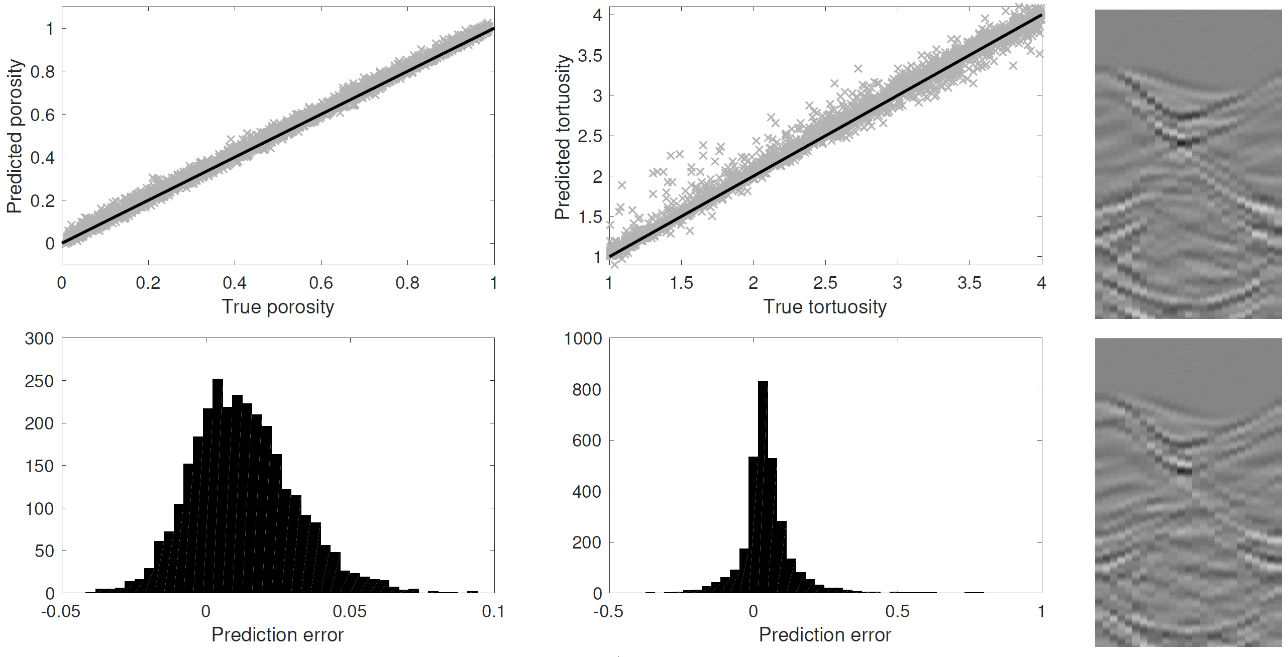
Figure 9: Predicted porosities (left) and tortuosities (middle) for the test data with white noise of 0.8% (relative to the maximum absolute value of the signal in the training set). Bottom row (left and middle) shows histograms of the prediction error (difference between the predicted and true values). The right column shows two examples of the sample images in this noise level.

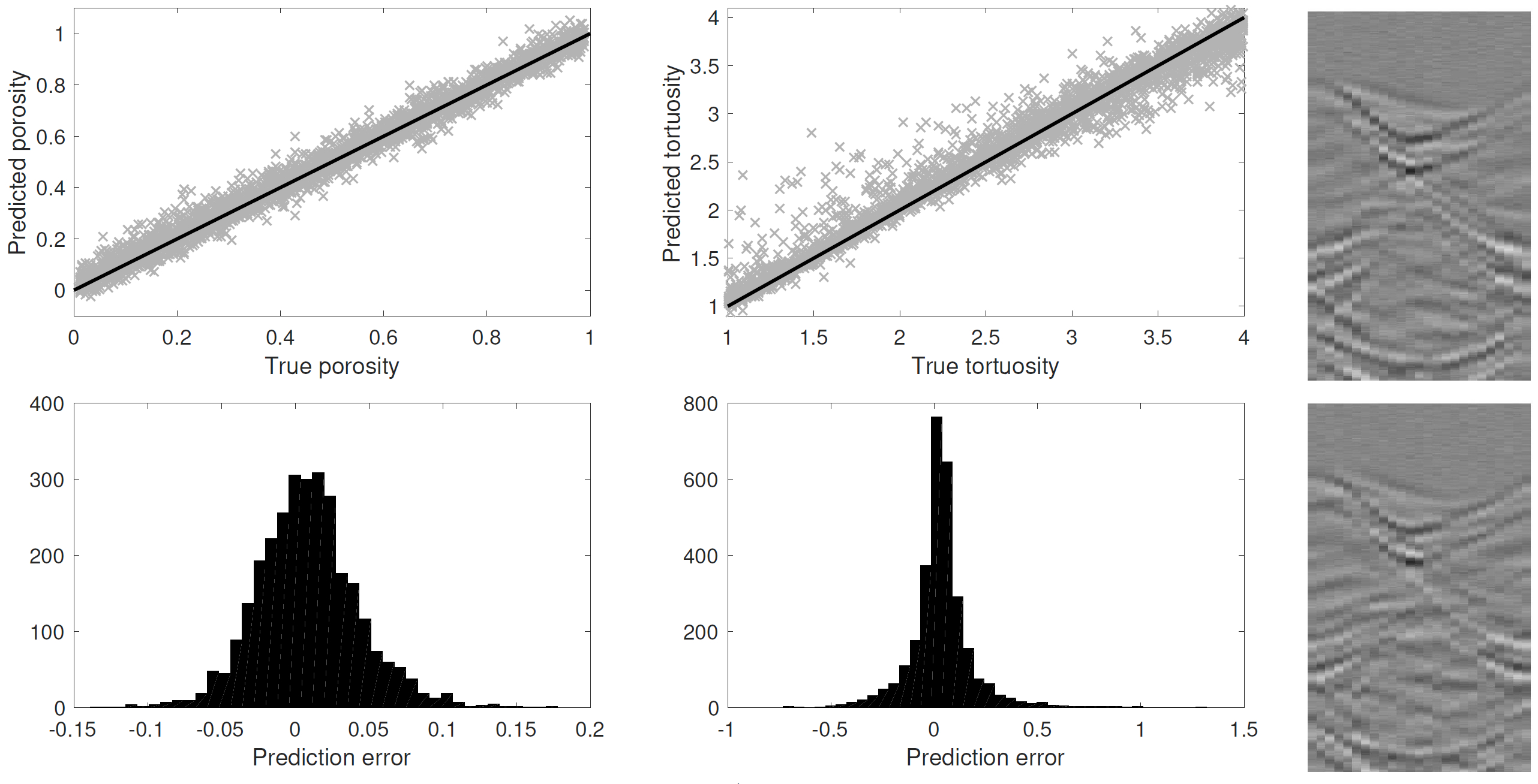
Figure 10: Predicted porosities (left) and tortuosities (middle) for the test data with white noise of 3.2% (relative to the maximum absolute value of the signal in the training set). Bottom row (left and middle) shows histograms of the prediction error (difference between the predicted and true values). The right column shows two examples of the sample images in this noise level.

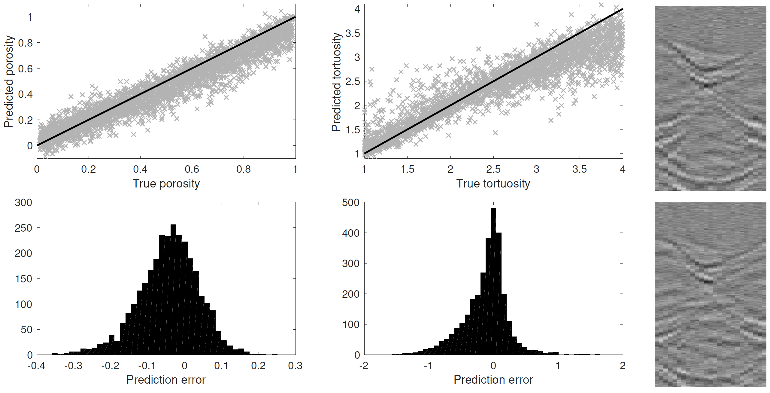
Figure 11: Predicted porosities (left) and tortuosities (middle) for the test data with white noise of 8.1% (relative to the maximum absolute value of the signal in the training set). Bottom row (left and middle) shows histograms of the prediction error (difference between the predicted and true values). The right column shows two examples of the sample images in this noise level.

Table 5: Bias, standard deviation, kurtosis and percentiles (25% and 75%) for the errors of the predicted porosities and tortuosities with different noise levels.

Noise	Porosity					Tortuosity
level	Bias	S.D.	Kurtosis	25%	75%	Bias	S.D.	Kurtosis	25%	75%
0 %	0.012	0.016	3.2	0.0011	0.023	0.041	0.087	14	0.0092	0.07
0.16 %	0.012	0.016	3.2	0.0012	0.023	0.042	0.087	14	0.0097	0.07
0.49 %	0.013	0.017	3.3	0.0013	0.023	0.044	0.091	15	0.0087	0.073
0.81 %	0.013	0.018	3.5	0.00078	0.024	0.046	0.096	15	0.0076	0.075
1.6 %	0.013	0.023	4.1	-0.002	0.026	0.047	0.11	14	0.0016	0.08
3.2 %	0.0087	0.035	4.4	-0.014	0.028	0.035	0.16	11	-0.026	0.085
4.9 %	-0.0029	0.049	4.2	-0.034	0.027	-0.0012	0.22	8.1	-0.085	0.082
8.1%	-0.043	0.081	3.6	-0.093	0.0099	-0.12	0.34	5.1	-0.29	0.062

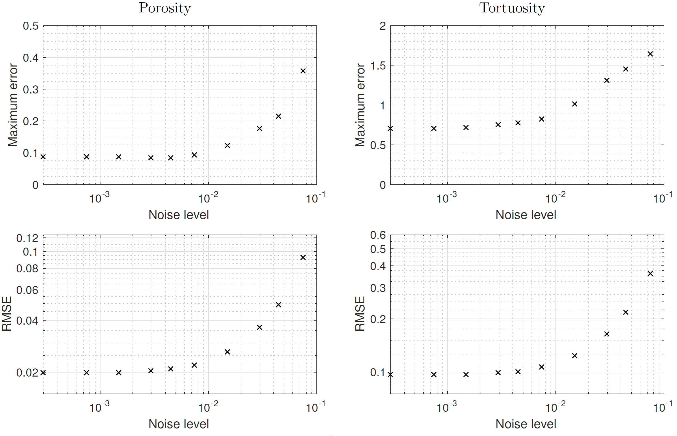
Figure 12: The maximum absolute errors and the root-mean-square errors (RMSE) as a function of the noise level. The x-axis is the noise level relative to the maximum of the (noise-free) signal in the training set.

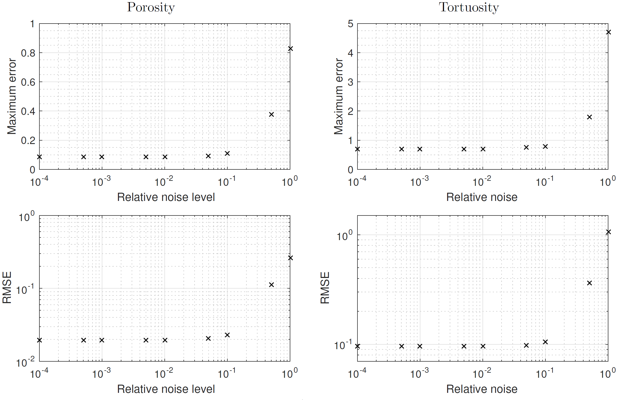
Figure 13: The maximum absolute errors and the root-mean-square errors (RMSE) as a function of the relative noise ($B$ in Eq. (18)).

5 CONCLUSIONS

In this paper, we proposed the use of convolutional neural networks (CNN) for estimation of porous material parameters from synthetic ultrasound tomography data. In the studied model, ultrasound data was generated in a water tank into which the poroelastic material sample was placed. A total of 26 ultrasound sensors were positioned in the water. One of the sensors generated the source pulse while others were used in the receiving mode. The recorded velocity data were represented as images which were further used as an input to the CNN.

In the experiment, the parameter space for the porous inclusion was assumed to be large. For example, the porosity of the inclusion was allowed to span the interval from 1% to 99%. The selected parameter space models a different type of materials. We estimated the porosity and tortuosity of the porous material sample while all other material parameters were considered as nuisance parameters (see Table 1). Based on the results, it seems that these parameters can be estimated with acceptable accuracy with a wide variety of noise levels, while the nuisance parameters are successfully marginalized. The error histograms for both porosity and tortuosity show excellent accuracy in terms of root-mean-square error and bias.

We have marginalized our inference of porosity and tortuosity over 6 other material parameters (listed in Table 1), which makes it possible to detect the primary porous material parameters from the waveforms without the knowledge of the values of the nuisance parameters, even if they can have a significant impact on the waveforms themselves. The success in the marginalization significantly increases the potential of the neural networks for material characterization.

Future studies should include more comprehensive investigation of model uncertainties including geometrical inaccuracies (positioning and size of the material sample), fluid parameter changes, viscoelastic parameters of the shell layer, material inhomogeneities, and the sensor setup. In addition, the extension to three spatial dimensions together with actual measurements are essential steps to guarantee the effectiveness of the proposed method.

Acknowledgments

This work has been supported by the strategic funding of the University of Eastern Finland and by the Academy of Finland (project 250215, Finnish Centre of Excellence in Inverse Problems Research). This article is based upon work from COST Action DENORMS CA-15125, supported by COST (European Cooperation in Science and Technology).

References

- [1] N. Duric, P. J. Littrup, C. Li, O. Roy, and S. Schmidt, “Ultrasound tomography: A decade-long journey from the laboratory to clinic,” in Ultrasound Imaging and Therapy, edited by A. Karellas and B. R. Thomadsen (CRC Press, Taylor & Francis Group, 2015).
- [2] M. Biot, “Theory of propagation of elastic waves in a fluid saturated porous solid. I. Low frequency range,” J. Acoust. Soc. Am. 28(2), 168–178 (1956).
- [3] M. Biot, “Theory of propagation of elastic waves in a fluid saturated porous solid. II. Higher frequency range,” J. Acoust. Soc. Am. 28(2), 179–191 (1956).
- [4] M. Biot, “Mechanics of deformation and acoustic propagation in porous media,” J. Appl. Phys. 33(4), 1482–1498 (1962).
- [5] M. Biot, “Generalized theory of acoustic propagation in porous dissipative media,” J. Acoust. Soc. Am. 34(5), 1254–1264 (1962).
- [6] N. Sebaa, Z. Fellah, M. Fellah, E. Ogam, A. Wirgin, F. Mitri, C. Depollier, and W. Lauriks, “Ultrasonic characterization of human cancellous bone using the Biot theory: Inverse problem,” J. Acoust. Soc. Am. 120(4), 1816–1824 (2006).
- [7] M. Yvonne Ou, “On reconstruction of dynamic permeability and tortuosity from data at distinct frequencies,” Inverse Problems 30(9), 095002 (2014).
- [8] T. Lähivaara, N. Dudley Ward, T. Huttunen, Z. Rawlinson, and J. Kaipio, “Estimation of aquifer dimensions from passive seismic signals in the presence of material and source uncertainties,” Geophys. J. Int. 200, 1662–1675 (2015).
- [9] J. Parra Martinez, O. Dazel, P. Göransson, and J. Cuenca, “Acoustic analysis of anisotropic poroelastic multilayered systems,” J. Appl. Phys. 119(8), 084907 (2016).
- [10] A. Krizhevsky, I. Sutskever, and G. Hinton, “Imagenet classification with deep convolutional neural networks,” in Advances in Neural Information Processing Systems 25, edited by F. Pereira, C. J. C. Burges, L. Bottou, and K. Q. Weinberger (Curran Associates, Inc., 2012), pp. 1097–1105.
- [11] Y. LeCun, Y. Bengio, and G. Hinton, “Deep learning,” Nature 521(7553), 436–444 (2015).
- [12] P. S. Maclin, J. Dempsey, J. Brooks, and J. Rand, “Using neural networks to diagnose cancer,” J. Med. Syst. 15(1), 11–19 (1991).
- [13] L. A. Menendez, F. J. de Cos Juez, F. S. Lasheras, and J. A. Riesgo, “Artificial neural networks applied to cancer detection in a breast screening programme,” Math. Comput. Model. 52(7-8), 983–991 (2010).
- [14] P. Muukkonen and J. Heiskanen, “Estimating biomass for boreal forests using ASTER satellite data combined with standwise forest inventory data,” Remote Sens. Environ. 99(4), 434–447 (2005).
- [15] H. Niska, J.-P. Skön, P. Packalen, T. Tokola, M. Maltamo, and M. Kolehmainen, “Neural networks for the prediction of species-specific plot volumes using airborne laser scanning and aerial photographs,” IEEE Trans. Geosci. Remote Sens. 48(3), 1076–1085 (2009).
- [16] I. N. Daliakopoulos, P. Coulibaly, and I. K. Tsanis, “Groundwater level forecasting using artificial neural networks,” J. Hydrol. 309(1-4), 229–240 (2005).
- [17] S. Mohanty, K. Jha, A. Kumar, and K. P. Sudheer, “Artificial neural network modeling for groundwater level forecasting in a River Island of Eastern India,” Water Resour. Manage. 24(9), 1845–1865 (2010).
- [18] Y. LeCun, L. Bottou, Y. Bengio, and P. Haffner, “Gradient-based learning applied to document recognition,” Proceedings of the IEEE 86(11), 2278–2324 (1998).
- [19] Y. Bengio, “Learning deep architectures for AI,” Found. Trends Mach. Learn. 2(1), 1–127 (2009).
- [20] J. Carcione, Wave Fields in Real Media: Wave propagation in anisotropic, anelastic and porous media (Elsevier, 2001).
- [21] C. Morency and J. Tromp, “Spectral-element simulations of wave propagation in porous media,” Geophys. J. Int. 175(1), 301–345 (2008).
- [22] L. Wilcox, G. Stadler, C. Burstedde, and O. Ghattas, “A high-order discontinuous Galerkin method for wave propagation through coupled elastic-acoustic media,” J. Comput. Phys. 229, 9373–9396 (2010).
- [23] N. Dudley Ward, T. Lähivaara, and S. Eveson, “A discontinuous Galerkin method for poroelastic wave propagation: Two-dimensional case,” J. Comput. Phys. 350, 690–727 (2017).
- [24] M. Käser and M. Dumbser, “An arbitrary high-order discontinuous Galerkin method for elastic waves on unstructured meshes - I. The two-dimensional isotropic case with external source terms,” Geophys. J. Int. 166(23), 855–877 (2006).
- [25] J. de la Puente, M. Dumbser, M. Käser, and H. Igel, “Discontinuous Galerkin methods for wave propagation in poroelastic media,” Geophysics 73(5), T77–T97 (2008).
- [26] G. Gabard and O. Dazel, “A discontinuous Galerkin method with plane waves for sound-absorbing materials,” Int. J. Numer. Meth. Eng. 104(12), 1115–1138 (2015).
- [27] J. Hesthaven and T. Warburton, Nodal Discontinuous Galerkin Methods: Algorithms, Analysis, and Applications (Springer, 2007).
- [28] N. Buduma, Fundamentals of Deep Learning, Designing Next-Generation Machine Intelligence Algorithms (O’Reilly Media, 2017).
- [29] R. Hahnloser, M.A.Sarpeshkar, M. A. Mahowald, R. J. Douglas, and H.S.Seung, “Digital selection and analogue amplification coexist in a cortex-inspired silicon circuit,” Nature 405, 947-951 (2000).
- [30] K. Fukushima, “Neocognitron: A self-organizing neural network model for a mechanism of pattern recognition unaffected by shift in position,” Biological Cybernetics 36, 93–202 (1980).
- [31] D. Scherer, A. Müller, and S. Behnke, Evaluation of Pooling Operations in Convolutional Architectures for Object Recognition, 92–101 (Springer Berlin Heidelberg, Berlin, Heidelberg).
- [32] S. Linnainmaa, “The representation of the cumulative rounding error of an algorithm as a Taylor expansion of the local rounding errors (in finnish),” Master’s thesis, University of Helsinki, http://people.idsia.ch/~juergen/linnainmaa1970thesis.pdf (1970).
- [33] M. Carpenter and C. Kennedy, Fourth-order 2N-storage Runge-Kutta schemes (Technical report, NASA-TM-109112, 1994).
- [34] E. Blanc, D. Komatitsch, E. Chaljub, B. Lombard, and Z. Xie, “Highly accurate stability-preserving optimization of the Zener viscoelastic model, with application to wave propagation in the presence of strong attenuation,” Geophys. J. Int. 205(1), 427–439 (2016).
- [35] T. Lähivaara and T. Huttunen, “A non-uniform basis order for the discontinuous Galerkin method of the acoustic and elastic wave equations,” Appl. Numer. Math. 61, 473–486 (2011).
- [36] T. Lähivaara and T. Huttunen, “A non-uniform basis order for the discontinuous Galerkin method of the 3D dissipative wave equation with perfectly matched layer,” J. Comput. Phys. 229, 5144–5160 (2010).
- [37] J. Kaipio and E. Somersalo, “Statistical inverse problems: Discretization, model reduction and inverse crimes,” J. Comput. Appl. Math. 198(2), 493–504 (2007).
- [38] D. Kingma and J. Ba, “Adam: A Method for Stochastic Optimization,” ArXiv e-prints (2014).