A Blob Method For Diffusion
Abstract.
As a counterpoint to classical stochastic particle methods for diffusion, we develop a deterministic particle method for linear and nonlinear diffusion. At first glance, deterministic particle methods are incompatible with diffusive partial differential equations since initial data given by sums of Dirac masses would be smoothed instantaneously: particles do not remain particles. Inspired by classical vortex blob methods, we introduce a nonlocal regularization of our velocity field that ensures particles do remain particles and apply this to develop a numerical blob method for a range of diffusive partial differential equations of Wasserstein gradient flow type, including the heat equation, the porous medium equation, the Fokker–Planck equation, and the Keller–Segel equation and its variants. Our choice of regularization is guided by the Wasserstein gradient flow structure, and the corresponding energy has a novel form, combining aspects of the well-known interaction and potential energies. In the presence of a confining drift or interaction potential, we prove that minimizers of the regularized energy exist and, as the regularization is removed, converge to the minimizers of the unregularized energy. We then restrict our attention to nonlinear diffusion of porous medium type with at least quadratic exponent. Under sufficient regularity assumptions, we prove that gradient flows of the regularized porous medium energies converge to solutions of the porous medium equation. As a corollary, we obtain convergence of our numerical blob method. We conclude by considering a range of numerical examples to demonstrate our method’s rate of convergence to exact solutions and to illustrate key qualitative properties preserved by the method, including asymptotic behavior of the Fokker–Planck equation and critical mass of the two-dimensional Keller–Segel equation.
2010 Mathematics Subject Classification:
35Q35 35Q82 65M12 82C22;Key words and phrases. Particle method, porous medium equation, Wasserstein gradient flow, vortex blob method
1. Introduction
For a range of partial differential equations, from the heat and porous medium equations to the Fokker–Planck and Keller–Segel equations, solutions can be characterized as gradient flows with respect to the quadratic Wasserstein distance. In particular, solutions of the equation
| (1) |
where is a curve in the space of probability measures, are formally Wasserstein gradient flows of the energy
| (2) |
where is -dimensional Lebesgue measure. This implies that solutions of (1) satisfy
for a generalized notion of gradient , which is formally given by
where is the first variation density of at (c.f. [83, 28, 3, 29]).
Over the past twenty years, the Wasserstein gradient flow perspective has led to several new theoretical results, including asymptotic behavior of solutions of nonlinear diffusion and aggregation-diffusion equations [71, 28, 29], stability of steady states of the Keller–Segel equation [10, 12], and uniqueness of bounded solutions [27]. The underlying gradient flow theory has been well developed in the case of convex (or, more generally, semiconvex) energies [56, 83, 84, 3, 2, 5, 25, 78], and more recently, is being extended to consider energies with more general moduli of convexity [36, 29, 27, 6].
Wasserstein gradient flow theory has also inspired new numerical methods, with a common goal of maintaining the gradient flow structure at the discrete level, albeit in different ways. Recent work has considered finite volume, finite element, and discontinuous Galerkin methods [9, 17, 22, 81, 62]. Such methods are energy decreasing, positivity preserving, and mass conserving at the semidiscrete level, leading to high-order approximations. They naturally preserve stationary states, since dissipation of the free energy provides inherent stability, and often also capture the rate of asymptotic decay. Another common strategy for preserving the gradient flow structure at the discrete level is to leverage the discrete-time variational scheme introduced by Jordan, Kinderlehrer, and Otto [56]. A wide variety of strategies have been developed for this approach: working with different discretizations of the space of Lagrangian maps [43, 69, 70, 68, 57], using alternative formulations of the variational structure [44], making use of convex analysis and computational geometry to solve the optimality conditions [8], and many others [49, 48, 11, 30, 18, 32, 85, 24].
In this work, we develop a deterministic particle method for Wasserstein gradient flows. The simplest implementation of a particle method for equation (1), in the absence of diffusion, begins by first discretizing the initial datum as a finite sum of Dirac masses, that is,
| (3) |
where is a Dirac mass centered at . Without diffusion and provided sufficient regularity of and , the solution of (1) with initial datum remains a sum of Dirac masses at all times , so that
| (4) |
and solving the partial differential equation (1) reduces to solving a system of ordinary differential equations for the locations of the Dirac masses,
| (5) |
The particle solution is the Wasserstein gradient flow of the energy (2) with initial data , so in particular the energy decreases in time along this spatially discrete solution. The ODE system (5) can be solved using range of fast numerical methods, and the resulting discretized solution can be interpolated in a variety of ways for graphical visualization.
This simple particle method converges to exact solutions of equation (1) under suitable assumptions on and , as has been shown in the rigorous derivation of this equation as the mean-field limit of particle systems [23, 25, 53]. Recent work, aimed at capturing competing effects in repulsive-attractive systems and developing methods with higher-order accuracy, has considered enhancements of standard particle methods inspired by techniques from classical fluid dynamics, including vortex blob methods and linearly transformed particle methods [47, 50, 37, 20]. Bertozzi and the second author’s blob method for the aggregation equation obtained improved rates of convergence to exact solutions for singular interaction potentials by convolving with a mollifier . In terms of the Wasserstein gradient flow perspective this translates into regularizing the interaction energy as .
When diffusion is present in equation (1), the fundamental assumption underlying basic particle methods breaks down: particles do not remain particles, or in other words, the solution of (1) with initial datum (3) is not of the form (4). A natural way to circumvent this difficulty, at least in the case of linear diffusion (), is to consider a stochastic particle method, in which the particles evolve via Brownian motion. Such approaches were originally developed in the classical fluids case [34], and several recent works have considered analogous methods for equations of Wasserstein gradient flow type, including the Keller–Segel equation [53, 54, 63, 51]. The main practical disadvantage of these stochastic methods is that their results must be averaged over a large number of runs to compensate for the inherent randomness of the approximation. Furthermore, to the authors’ knowledge, such methods have not been extended to the case of degenerate diffusion .
Alternatives to stochastic methods have been explored for similar equations, motivated by particle-in-cell methods in classical fluid, kinetic, and plasma physics equations. These alternatives proceed by introducing a suitable regularization of the flux of the continuity equation [76, 35]. Degond and Mustieles considered the case of linear diffusion () by interpreting the Laplacian as induced by a velocity field , , , and regularizing the numerator and denominator separately by convolution with a mollifier [41, 75]. For this regularized equation, particles do remain particles, and a standard particle method can be applied. Well-posedness of the resulting system of ordinary differential equations and a priori estimates relevant to the method were studied by Lacombe and Mas-Gallic [59] and extended to the case of the porous medium equation by Oelschläger and Lions and Mas-Gallic [67, 61, 64]. In the case on bounded domains, Lions and Mas-Gallic succeeded in showing that solutions to the regularized equation converge to solutions of the unregularized equation, as long as the initial data has uniformly bounded entropy. Unfortunately, this assumption fails to hold when the initial datum is given by a particle approximation (3), and consequently Lions and Mas-Gallic’s result doesn’t guarantee convergence of the particle method. Oelschläger [67], on the other hand, succeeded in proving convergence of the deterministic particle method, as long as the corresponding solution of the porous medium equation is smooth and positive. An alternative approach, now known as the particle strength exchange method, incorporates instead the effects of diffusion by allowing the weights of the particles to vary in time. Degond and Mas-Gallic developed such a method for linear diffusion () and proved second order convergence with respect to the initial particle spacing [40, 39]. The main disadvantage of these existing deterministic particle methods is that, with the exception of Lions and MasGallic’s work when , they do not preserve the gradient flow structure [61]. Other approaches that respect the method’s variational structure have been recently proposed in one dimension by approximating particles by non-overlapping blobs [26, 31]. For further background on deterministic particle methods, we refer the reader to Chertock’s comprehensive review [33].
The goal of the present paper is to introduce a new deterministic particle method for equations of the form (1), with linear and nonlinear diffusion (), that respects the problem’s underlying gradient flow structure and naturally extends to all dimensions. In contrast to the above described work, which began by regularizing the flux of the continuity equation, we follow an approach analogous to Bertozzi and the second author’s blob method for the aggregation equation and regularize the associated internal energy . For a mollifier , , , we define
| (6) |
For more general nonlinear diffusion, we define
| (7) |
As , we prove that the regularized internal energies -converge to the unregularized energies for all ; see Theorem 4.1. In the presence of a confining drift or interaction potential, so that minimizers exist, we also show that minimizers converge to minimizers; see Theorem 4.5. For and semiconvex potentials , we show that the gradient flows of the regularized energies are well-posed and are characterized by solutions to the partial differential equation
| (8) |
Under sufficient regularity conditions, we prove that solutions of the regularized gradient flows converge to solutions of equation (1); see Theorem 5.8. When and the initial datum has bounded entropy, we show that these regularity conditions automatically hold, thus generalizing Lions and Mas-Gallic’s result for the porous medium equation on bounded domains to the full equation (1) on all of ; see Corollary 5.9 and [61, Theorem 2].
For this regularized equation (8), particles do remain particles; see Corollary 5.5. Consequently, our numerical blob method for diffusion consists of taking a particle approximation for (8). We conclude by showing that, under sufficient regularity conditions, our blob method’s particle solutions converge to exact solutions of (1); see Theorem 6.1. We then give several numerical examples illustrating the rate of convergence of our method and its qualitative properties.
A key advantage of our approach is that, by regularizing the energy functional and not the flux, we preserve the problem’s gradient flow structure. Still, at first glance, our regularization of the energy (6) may seem less natural than other potential choices. For example, one could instead consider the following more symmetric regularization
for more general nonlinear diffusion,
Although studying the above regularization is not without interest, we focus our attention on the regularization in (6) and (7) for numerical reasons. Indeed, computing the first variation density of gives
as compared to
for . In the first case, one can see that replacing by a sum of Dirac masses still requires the computation of an integral convolution with . Indeed, if , where are particles in with masses , then, for all ,
which does not allow for a complete discretization of the integrals. On the contrary, in the second case, all convolutions involve , so a similar computation (as it can be found in the proof of Corollary 5.5) shows that they reduce to finite sums, which are numerically less costly.
Another advantage of our approach, in the case, is that our regularization of the energy can naturally be interpreted as an approximation of the porous medium equation by a very localized nonlocal interaction potential. In this way, our proof of the convergence of the associated particle method provides a theoretical underpinning to approximations of this kind in the computational math and swarming literature [60, 58]. Further advantages our blob method include the ease with which it may be combined with particle methods for interaction and drift potentials, its simplicity in any dimension, and the good numerical performance we observe for a wide choice of interaction and drift potentials.
Our paper is organized as follows. In Section 2, we collect preliminary results concerning the regularization of measures via convolution with a mollifier, including a mollifier exchange lemma (Lemma 2.2), and relevant background on Wasserstein gradient flow and weak convergence of measures. In Section 3, we prove several results on the general regularized energies (7), which are of a novel form from the perspective of Wasserstein gradient flow theory, combining aspects of the well-known interaction and internal energies. We show that these regularized energies are semiconvex and differentiable in the Wasserstein metric and characterize their subdifferential with respect to this structure; see Propositions 3.10–3.12. In Section 4, we prove that -converges to as and that minimizers converge to minimizers, when in the presence of a confining drift or interaction term; see Theorems 4.1 and 4.5. With this -convergence in hand, in Section 5 we then turn to the question of convergence of gradient flows, restricting to the case . Using the framework introduced by Sandier and Serfaty [79, 77], we prove that, under sufficient regularity assumptions, gradient flows of the regularized energies converge as to gradient flows of the unregularized energy, recovering a generalization of Lions and Mas-Gallic’s results when ; see Theorem 5.8 and Corollary 5.9. Finally, in Section 6, we prove the convergence of our numerical blob method, under sufficient regularity assumptions, when the initial particle spacing scales with the regularization like ; see Theorem 6.1.
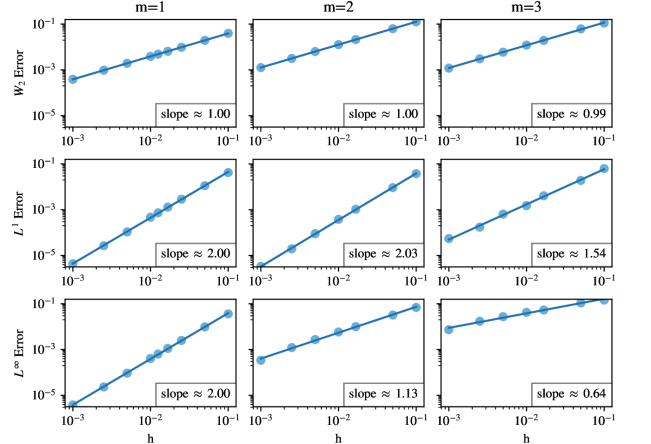
We close with several numerical examples, in one and two dimensions, analyzing the rate of convergence to exact solutions with respect to the -Wasserstein metric, -norm, and -norm and illustrating qualitative properties of the method, including asymptotic behavior of the Fokker–Planck equation and critical mass of the two-dimensional Keller–Segel equation; see Section 6.3. In particular, for the heat equation and porous medium equations (, ), we observe that the -Wasserstein error depends linearly on the grid spacing for , while the -norm depends quadratically on the grid spacing for and superlinearly for . We apply our method to study long time behavior of the nonlinear Fokker–Planck equation (, , ), showing that the blob method accurately captures convergence to the unique steady state. Finally, we conduct a detailed numerical study of equations of Keller–Segel type, including a one-dimensional variant () and the original two-dimensional equation (, , ). The one-dimensional equation has a critical mass , and the two-dimensional equation has critical mass , at which point the concentration effects from the nonlocal interaction term balance with linear diffusion () [42, 13]. We show that the same notion of criticality is present in our numerical solutions and demonstrate convergence of the critical mass as the grid spacing and regularization are refined.
There are several directions for future work. Our convergence theorem for requires additional regularity assumptions, which we are only able to remove in the case when the initial data has bounded entropy. In the case of or more general initial data, it remains an open question how to control certain nonlocal norms of the regularized energies, which play an important role in our convergence result; see Theorem 5.8. Formally, we expect these to behave as approximations of the -norm of , which should remain bounded by the gradient flow structure; see equations (24) and (25). When , it is not clear how to use these nonlocal norms to get the desired convergence result or whether an entirely different approach is needed. Perhaps related to these questions is the fact that our estimate on the semiconvexity of the regularized energies (6) deteriorates as , while we expect that the semiconvexity should not deteriorate along smooth geodesics; see Proposition 3.11. Finally, while our results show convergence of the blob method for diffusive Wasserstein gradient flows, they do not quantify the rate of convergence in terms of and . In particular, a theoretical result on the optimal scaling relation between and remains open, though we observe good numerical performance for , . In a less technical direction, we foresee a use of the presented ideas in conjunction with splitting schemes for certain nonlinear kinetic equations [21, 1], as well as in the fluids [50], since our numerical results demonstrate comparable rates of convergence to the particle strength exchange method, which has already gained attention in these contexts [41].
2. Preliminaries
2.1. Basic notation
For any and we denote the open ball of center and radius by . Given a set , we write for the indicator function of , i.e., for and otherwise. We say a function has at most quadratic growth if there exist so that for all .
Let denote the set of Borel probability measures on , and for, any , denotes elements of with finite th moment, . We write for the -dimensional Lebesgue measure, and for given , we write if is absolutely continuous with respect to the Lebesgue measure. Often we use the same symbol for both a probability measure and its Lebesgue density, whenever the latter exists. We let denote the Lebesgue space of functions with th power integrable against .
Given a finite, signed Borel measure on , we denote its variation by . For a Borel set we write for the -measure of set . For a Borel map and , we write for the push-forward of through . We let denote the identity map on and define by for all . For a sequence and some , we write if converges to in the weak-∗ topology of probability measures, i.e., in the duality with bounded continuous functions.
2.2. Convolution of measures
A key aspect of our approach is the regularization of the energy (2) via convolution with a mollifier. In this section, we collect some elementary results on the convolution of probability measures, including a mollifier exchange lemma, Lemma 2.2.
For any and measurable function , the convolution of with is given by
whenever the integral converges. We consider mollifiers satisfying the following assumption.
ASSUMPTION 2.1 (mollifier).
Let , where is even, , and
This assumption is satisfied by both Gaussians and smooth functions with compact support. Assumption 2.1 also ensures that has finite first moment. For any , we write
Throughout, we use the fact that the definition of convolution allows us to move mollifiers from the measure to the integrand. In particular, for any bounded below and even,
Likewise, the technical assumption that , and therefore that , allows us to regularize integrands involving the mollifier ; indeed, the following lemma provides sufficient conditions for moving functions in and out convolutions with mollifiers within integrals. (See also [61] for a similar result.) This is an essential component in the proofs of both main results, Theorems 4.1 and 5.8, on the the -convergence of the regularized energies and the convergence of the corresponding gradient flows. See Appendix A for the proof of this lemma.
LEMMA 2.2 (mollifier exchange lemma).
Let be Lipschitz continuous with Lipschitz constant , and let and be finite, signed Borel measures on . There is so that
We conclude this section with a lemma stating that if a sequence of measures converges in the weak-∗ topology of , then the mollified sequence converges to the same limit. We refer the reader to Appendix A for the proof.
LEMMA 2.3.
Let be a sequence in such that as for some . Then .
2.3. Optimal transport, Wasserstein metric, and gradient flows
We now describe basic facts about optimal transport, including the Wasserstein metric and associated gradient flows. (See also [3, 83, 78, 84, 2, 5] for further background and more details on the definitions and remarks found in this section.)
For , we denote the set of transport plans from to by
where are the projections of onto the first and second copy of , respectively. The Wasserstein distance between two probability measures is given by
| (9) |
and a transport plan is optimal if it attains the minimum in (9). We denote the set of optimal transport plans by . If is absolutely continuous with respect to the Lebesgue measure, then there is a unique optimal transport plan , and
for a Borel measurable function . is unique up to sets of -measure zero and is known as the optimal transport map from to . Convergence with respect to the Wasserstein metric is stronger than weak-∗ convergence. In particular, if and , then
In order to define Wasserstein gradient flows, we will require the following notion of regularity in time with respect to the Wasserstein metric.
DEFINITION 2.4 (absolutely continuous).
if there is so that
Along such curves, we have a notion of metric derivative.
DEFINITION 2.5 (metric derivative).
Given , its metric derivative is
An important class of curves in the Wasserstein metric are the (constant speed) geodesics. Given , geodesics connecting to are of the form
If is induced by a map , then
More generally, given , a generalized geodesic connecting to with base is given by
| (10) | ||||
with the projection of onto the first and th copies of . When the base coincides with one of the endpoints or , generalized geodesics are geodesics.
A key property for the uniqueness and stability of Wasserstein gradient flows is that the energies are convex, or more generally semiconvex, along generalized geodesics.
DEFINITION 2.6 (semiconvexity along generalized geodesics).
We say a functional is semiconvex along generalized geodesics if there is such that for all there exists a generalized geodesic connecting to with base such that
where
For any subset and functional , we denote the domain of by , and we say that is proper if . As soon as a functional is proper and lower semicontinuous with respect to the weak-* topology, we may define its subdifferential; see [3, Definition 10.3.1 and Equation 10.3.12]. Following the approach in [25], the notion of subdifferential we use in this paper is, in fact, the following reduced one.
DEFINITION 2.7 (subdifferential).
Given proper and lower semicontinuous, , and with , then belongs to the subdifferential of at , written , if as ,
The Wasserstein metric is formally Riemannian, and we may define the tangent space as follows.
DEFINITION 2.8.
Let . The tangent space at is
where the closure is taken in .
We now turn to the definition of a gradient flow in the Wasserstein metric (c.f. [3, Proposition 8.3.1, Definition 11.1.1]).
DEFINITION 2.9 (gradient flow).
Suppose is proper and lower semicontinuous. A curve is a gradient flow of if there exists a velocity vector field with for almost every such that is a weak solution of the continuity equation
i.e., is a solution to the continuity equation in duality with .
We close this section with the following definition of the Wasserstein local slope.
DEFINITION 2.10 (local slope).
Given , its local slope is
where the subscript denotes the positive part.
3. Regularized internal energies
The foundation of our blob method is the regularization of the internal energy via convolution with a mollifier. This allows us to preserve the gradient flow structure and approximate our original partial differential equation (1) by a sequence of equations for which particles do remain particles. In this section, we consider several fundamental properties of the regularized internal energies , including convexity, lower semicontinuity, and differentiability. In what follows, we will suppose that our internal energies satisfy the following assumption.
ASSUMPTION 3.1 (internal energies).
Suppose satisfies and either is bounded below or for some . Suppose further that is convex, bounded below, and .
Thanks to this assumption we can define the internal energy corresponding to by
If is bounded below, this is well-defined on all of . If for some , this is well-defined on ; see [3, Example 9.3.6].
REMARK 3.2 (nondecreasing).
Assumption 3.1 implies that is nondecreasing. Indeed, by the convexity of and the fact that ,
which leads to for all .
Our assumption does not ensure that is convex along Wasserstein geodesics, unless is convex.
REMARK 3.3 (McCann’s convexity condition).
We regularize the internal energies by convolution with a mollifier.
DEFINITION 3.4 (regularized internal energies).
Given satisfying Assumption 3.1, we define, for all , the regularized internal energies by
Note that, for all and , .
An important class of internal energies satisfying Assumption 3.1 are given by the (negative) entropy and Rényi entropies.
DEFINITION 3.5.
The entropy and Rényi entropies, and their regularizations, are given by
Note that, as per our observation just below the definition of , the entropy is well-defined on and the Rényi entropies () are well-defined on all of . Also note that the regularized entropies () are well-defined on all of .
In order to approximate solutions of equation (1), we will consider combinations of the above regularized internal energies with potential and interaction energies.
DEFINITION 3.6 (regularized energies).
Let be proper and lower semicontinuous. Suppose further that is locally integrable. For all define
When for some , then we denote by and by .
The regularized internal energy in Definition 3.4 incorporate a blend of interaction and internal phenomena, through the convolution with the mollifier, or potential, and the composition with the function . To our knowledge, this is a novel form of functional on the space of probability measures. We now describe some of its basic properties: energy bounds and lower semicontinuity, when is the logarithm or a power, and differentiability, convexity and subdifferential characterization when is convex. For the existence and uniqueness of gradient flows associated to this regularized energy, see Section 5.
REMARK 3.7.
Although the regularized energy in Definition 3.4 is of a novel form, it was noticed in [72, Proposition 6.9] that a previous particle method for diffusive gradient flows leads to a similar regularized internal energy after space discretization [31, 26]. The essential difference between these two methods stands in the choice of the mollifier, which, instead of satisfying 2.1, is a very singular potential.
We begin with inequalities relating the regularized internal energies to the unregularized energies. See Appendix A for the proof, which is a consequence of Jensen’s inequality and a Carleman-type estimate on the lower bound of the entropy [31, Lemma 4.1].
PROPOSITION 3.8.
Let . If , suppose , and if , suppose . Then,
| (11) | ||||
| (12) |
where as . Furthermore, for all , we have
| (13) |
For all , the regularized entropies are lower semicontinuous with respect to weak-* convergence () and Wasserstein convergence (). For , we prove this using a theorem of Ambrosio, Gigli, and Savaré on the convergence of maps with respect to varying measures; see Proposition B.2. For , this is a consequence of Jensen’s inequality. For , we apply both Jensen’s inequality and a version of Fatou’s lemma for varying measures; see Lemma B.3. In this case, we also require that the mollifier is a Gaussian, so that we can get the bound from below required by Fatou’s lemma. We refer the reader to Appendix A for the proof.
PROPOSITION 3.9 (lower semicontinuity).
Let . Then
-
(i)
is lower semicontinuous with respect to weak-∗ convergence in for all ;
-
(ii)
if is a Gaussian, then is lower semicontinuous with respect to the quadratic Wasserstein convergence in .
When is convex, the regularized internal energies are differentiable along generalized geodesics. The proof relies on the fact that is differentiable and , with bounded Hessian; see Appendix A.
PROPOSITION 3.10 (differentiability).
Let satisfy Assumption 3.1 and be convex. Given and with , let for . Then
| (14) |
A key consequence of the preceding proposition is that the regularized energies are semiconvex along generalized geodesics, as we now show.
PROPOSITION 3.11 (convexity).
Suppose satisfies Assumption 3.1 and is convex. Then is -convex along generalized geodesics, where
| (15) |
Proof.
We now use the previous results to characterize the subdifferential of the regularized internal energy. The structure of argument is classical (c.f. [56, 25, 3]), but due to the novel form of our regularized energies, we include the proof in Appendix A.
PROPOSITION 3.12 (subdifferential characterization).
As a consequence of this characterization of the subdifferential, we obtain the analogous result for the full energy , as in Definition 3.6. See Appendix A for the proof.
COROLLARY 3.13.
Suppose satisfies Assumption 3.1 and is convex. Let and . Suppose are semiconvex, with at most quadratic growth, and is even. Then
where
In particular, we have .
4. -convergence of regularized internal energies
We now turn to the convergence of the regularized energies and, when in the presence of confining drift or interaction terms, the corresponding convergence of their minimizers. In this section, and for the remainder of the work, we consider regularized entropies and Rényi entropies of the form for . We begin by showing that -converges to as with respect to the weak-∗ topology.
THEOREM 4.1 ( -converges to ).
If , consider and , and if , consider and .
-
(i)
If , we have .
-
(ii)
We have .
Proof.
We begin by showing the result for , in which case the function is concave. We first show part (i). By Proposition 3.8, for all ,
By Lemma 2.3, implies . Therefore, by the lower semicontinuity of with respect to weak-∗ convergence [3, Remark 9.3.8],
which gives the result. We now turn to part (ii). Again, by Proposition 3.8, for all ,
where as . Therefore, .
We now consider the case when . Part (ii) follows quickly: by Proposition 3.8, Young’s convolution inequality, and the fact that , for all we have
Taking the supremum limit as then gives the result. Let us prove part (i). Without loss of generality, we may suppose that is finite. Furthermore, there exists a positive sequence such that and . In particular, there exists for which for all . By Jensen’s inequality for the convex function and the fact that for all ,
Thus, since for all , we have . We now use this bound on the -norm of to deduce a stronger notion of convergence of to . First, since converges weakly-∗ to as , Lemma 2.3 ensures that converges weakly-∗ to . Since the -norm is lower semicontinuous with respect to weak-∗ convergence [66, Lemma 3.4], we have
so that . Furthermore, up to another subsequence, we may assume that converges weakly in . Also, since , for all we have
so converges weakly in to . By the Banach–Saks theorem (c.f. [74, Section 38]), up to taking a further subsequence of , the Cesàro mean defined by
converges to strongly in . Finally, for any , this ensures
so that
| (17) |
We now use this stronger notion convergence to conclude our proof of part (i). Since and
by part (i) of Proposition B.2, up to another subsequence, there exists so that for all ,
| (18) |
Furthermore, recalling the definition of the regularized energy and applying [3, Theorem 5.4.4(ii)],
Therefore, to finish the proof, it suffices to show that for -almost every . By Lemma 2.2 and the fact that for all , there exists and so that for all ,
Combining this with equation (18), we obtain
| (19) |
Finally, using equation (17) and the definition of as a sequence of convex combinations of the family , for all with we have
Since the limit in (19) exists, it coincides with its Cesàro mean on the right-hand side of the above equation. Thus, for all with ,
This gives for -almost every , which completes the proof. ∎
Now, we add a confining drift or interaction potential to our internal energies, so that energy minimizers exist and we may apply the previous -convergence result to conclude that minimizers converge to minimizers. For the remainder of the section we consider energies of the form given in Definition 3.6, with the following additional assumptions on and to ensure that the energy is confining.
ASSUMPTION 4.2 (confining assumptions).
The potentials and are bounded below and one of the following additional assumptions holds:
| (CV) | |||
| (CV′) | |||
| (CW) |
Under these assumptions, the regularized energies are lower semicontinuous with respect to weak-∗ convergence () and Wasserstein convergence (), where for the latter we assume is a Gaussian (c.f. Proposition 3.9, and [3, Lemma 5.1.7], [66, Lemma 3.4] and [80, Lemma 2.2]).
REMARK 4.3 (tightness of sublevels).
We now prove existence of minimizers of , for all .
PROPOSITION 4.4.
Proof.
First suppose , so that and is bounded below. By Remark 4.3, if (CV) holds, then any minimizing sequence of has a subsequence that converges in the weak-∗ topology. Likewise, if (CW) holds, then any minimizing sequence of has a subsequence that, up to translation, converges in the weak-∗ topology. By lower semicontinuity of , the limits of minimizing sequences are minimizers of .
Now, suppose . By Proposition 3.8, for all and ,
Consequently, by the assumption in (CV′) and the fact that is bounded below by, say, , we can choose and obtain
| (20) |
Hence any minimizing sequence has uniformly bounded second moment. Thus, has a subsequence that converges in the weak-∗ topology to a limit with finite second moment. By the lower semicontinuity of the limit must be a minimizer of . ∎
Finally, we conclude that minimizers of the regularized energy converge to minimizers of the unregularized energy.
THEOREM 4.5 (minimizers converge to minimizers).
Suppose . If Assumption (CV) holds, then for any sequence such that is a minimizer of for all , we have, up to a subsequence, , where is minimizes . Alternatively, if Assumption (CW) holds, then we have , up to a subsequence and translation, where again minimizes .
Now suppose . If Assumption (CV′) holds and is a Gaussian, then for any sequence such that is a minimizer of for all , we have, up to a subsequence, , where minimizes .
Proof.
The proof is classical. We include it for completeness.
We only prove the result under Assumptions (CV)/(CV′) since the argument for (CW) is analogous. For any , since is a minimizer of we have that for all if , and for all if . Taking the infimum limit of the left-hand side and the supremum limit of the right-hand side, Theorem 4.1(ii) ensures that
| (21) |
Since is proper there exists if and if so that the right-hand side is finite. Thus, up to a subsequence, we may assume that is uniformly bounded. When , for all , and this implies that is uniformly bounded, so is tight. When , the inequality in (20) ensures that is uniformly bounded, so again is tight. Thus, up to a subsequence, converges weakly-∗ to a limit if and if . By Theorem 4.1(i) and the inequality in (21), we obtain
for all if and for all if . Therefore, is a minimizer of . ∎
REMARK 4.6 (convergence of minimizers).
One the main difficulties for improving the topology in which the convergence of the minimizers happen is that we do not control -norms of the regularized minimizing sequences due to the special form of our regularized energy. This is the main reason we only get weak-∗ convergence in the previous result and the main obstacle to improve results for the -convergence of gradient flows, as we shall see in the next section.
5. -convergence of gradient flows
We now consider gradient flows of the regularized energies , as in Definition 3.6, for and prove that, under sufficient regularity assumptions, gradient flows of the regularized energies converge to gradient flows of the unregularized energy as . For simplicity of notation, we often write and for when we refer jointly to the regularized and unregularized energies.
We begin by showing that the gradient flows of the regularized energies are well-posed, provided that and satisfy the following convexity and regularity assumptions.
ASSUMPTION 5.1 (convexity and regularity of and ).
The potentials are semiconvex, with at most quadratic growth, and is even. Furthermore, there exist so
REMARK 5.2 (-convexity).
More generally, our results naturally extend to drift and interaction energies that are merely -convex; see [36]. However, given that the main interest of the present work is approximation of diffusion, we prefer the simplicity of Assumption (5.1), as it allows us to focus our attention on the regularized internal energy.
PROPOSITION 5.3.
Proof.
It suffices to verify that is proper, coercive, lower semicontinuous with respect to -Wasserstein convergence, and semiconvex along generalized geodesics; c.f. [3, Theorem 11.2.1]. (See also [3, Equation (2.1.2b)] for the definition of coercive.) If , then is finite on all of , and if , then is proper. Thus, our assumptions on and ensure that is proper. Clearly is bounded below. Hence, since the semiconvexity of and ensures that their negative parts have at most quadratic growth, is coercive.
For , Proposition 3.9 ensures that is lower semicontinuous with respect to weak-∗ convergence, hence also -Wasserstein convergence. For , the unregularized internal energy is also lower semicontinuous with respect to weak-∗ and -Wasserstein convergence [66, Lemma 3.4]. Since and are lower semicontinuous and their negative parts have at most quadratic growth, the associated potential and interaction energies are lower semicontinuous with respect to -Wasserstein convergence [3, Lemma 5.1.7, Example 9.3.4]. Therefore, is lower semicontinuous for all .
For , Proposition 3.11 ensures that is semiconvex along generalized geodesics in . For , the unregularized internal energy is convex [66, Theorem 2.2]. For and semiconvex, the corresponding drift and interaction energies are semiconvex [3, Proposition 9.3.2], [25, Remark 2.9]. Therefore, the resulting regularized energy is semiconvex. ∎
In the case , gradient flows of the energies are characterized as solutions of the partial differential equation (1); c.f. [3, Theorems 10.4.13 and 11.2.1], [25, Theorem 2.12]. Now, we show that gradient flows of the regularized energies can also be characterized as solutions of a partial differential equation.
PROPOSITION 5.4.
Proof.
Suppose is the gradient flow of . Then, by Definition 2.9 and Corollary 3.13, is a weak solution to the continuity equation with velocity field (22). Conversely, suppose is a weak solution to the continuity equation with velocity field (22). By Corollary 3.13, for almost every . Furthermore, since for all , by [3, Theorem 8.3.1]. ∎
A consequence of the previous proposition is that, for the regularized energies , particles remain particles, i.e. a solution of the gradient flow with initial datum given by a finite sum of Dirac masses remains a sum of Dirac masses, and the evolution of the trajectories of the particles is given by a system of ordinary differential equations.
COROLLARY 5.5.
Let and , and let and satisfy Assumption 5.1. Fix . For , fix and satisfying . Then the ODE system
| (23) |
is well-posed for all . Furthermore, belongs to and is the gradient flow of with initial conditions .
Proof.
To see that (23) is well-posed, first note that the function
is Lipschitz. Likewise, Assumption 5.1 ensures and are continuous and one-sided Lipschitz. Therefore, the ODE system (23) is well-posed forward in time.
Now, suppose solves (23) with initial data on an interval , for some fixed . We abbreviate by the velocity field for in (23). For any test function , the fundamental theorem of calculus ensures that, for all ,
Combining this with (23), we obtain
Multiplying both sides by , summing over , and taking for gives
for as in (22). Therefore, is a weak solution of the continuity equation with velocity field . Furthermore, for all
by the continuity of , , and . Therefore, by Proposition 5.4, we conclude that and is the gradient flow of . ∎
We now turn to the -convergence of the gradient flows of the regularized energies, using the scheme introduced by Sandier–Serfaty [77] and then generalized by Serfaty [79], which provides three sufficient conditions for concluding convergence. We will use the following variant of Serfaty’s result, which allows for slightly weaker assumptions on the gradient flows of the regularized energies, but follows from the same argument as Serfaty’s original result. (See also Remark 2.11 on the correspondence between Wasserstein gradient flows and curves of maximal slope.)
THEOREM 5.6 (c.f. [79, Theorem 2]).
Let . Suppose that, for all , belongs to and is a gradient flow of with well-prepared initial data, i.e.,
| (S0) |
Suppose further that there exists a curve in such that, for almost every , and
-
(S1)
,
-
(S2)
,
-
(S3)
.
Then , and is a gradient flow of .
For simplicity of notation, in what follows we shall at times omit dependence on time when referring to curves in the space of probability measures.
In order to apply Serfaty’s scheme in the present setting to obtain -convergence of the gradient flows, a key assumption is that the following quantity is bounded uniformly in along the gradient flows of the regularized energies :
where we use the abbreviation . This quantity differs from merely by the placement of the absolute value sign:
| (24) |
Serfaty’s scheme allows one to assume, without loss of generality, that is bounded uniformly in for almost every , and Hölder’s inequality ensures that ; see Proposition 3.12. Consequently, we miss the bound we require on merely by placement of the absolute value sign in inequality (24).
Still, has a useful heuristic interpretation. Through the proof of Theorem 5.8, we obtain
| (25) |
see the inequality (33) and Proposition B.2. Consequently, one may think of as a nonlocal approximation of the -norm of the gradient of .
We begin with a technical lemma we shall use to prove the convergence of the gradient flows.
LEMMA 5.7.
Let and , and let and . Then for any Lipschitz function with constant , there exists so that
where is as in Assumption 2.1.
Proof.
We argue similarly as in Lemma 2.2. Let be Lipschitz with constant . Then,
By Assumption 2.1, is so that for for all . Choose so that
| (26) |
Now, we break the integral with respect to above into integrals over the domain and , bounding the above quantity by
First, we consider . Since, in the integral, , we obtain
Now, we consider . We apply the inequality in (52) to obtain with in the integral—the inequality in (26) ensures . Consequently,
where, in the last inequality, we use that and, by Jensen’s inequality for the concave function ,
| (27) |
Since , Jensen’s inequality gives
| (28) |
This gives the result by taking . ∎
With this technical lemma in hand, we now turn to the -convergence of the gradient flows.
THEOREM 5.8.
Let , and let and be as in Assumption 5.1. Fix and suppose that is a gradient flow of for all satisfying
| (A0) |
for some . Furthermore, suppose that the following hold:
-
(A1)
;
-
(A2)
there exists such that in as , and .
Then for almost every , , and is the gradient flow of with initial data .
Proof.
First, we note that for almost every . This follows from (A2), which ensures in , hence in distribution for almost every . Then, since in distribution for all , we obtain in distribution. Finally, since weak-* convergence and convergence in distribution are equivalent when and are both probability measures [3, Remark 5.1.6], we obtain for almost every .
It remains to verify conditions (S0), (S1), (S2), and (S3) from Theorem 5.6. Item (S0) holds by assumption (A0). Item (S1) follows by the same argument as in [38, Theorem 5.6]. Item (S2) is an immediate consequence of the fact that for almost every , our main -convergence Theorem 4.1, and the lower semicontinuity of the potential and interaction energies with respect to weak-∗ convergence [3, Lemma 5.1.7].
We devote the remainder of the proof to showing Condition (S3). We shall use the following fact throughout: combining Assumption (A2) with Proposition 3.8 implies that
| (29) |
To prove (S3) we may assume, without loss of generality, that is finite, so by Fatou’s lemma
| (30) |
so for almost every . In particular, up to taking subsequences, we may assume that, for almost every , is bounded uniformly in . By Corollary 3.13,
Furthermore, note that if
| (31) |
then ; c.f. [3, Theorem 10.4.13]. Thus, to prove (S3) it suffices to show that
| (32) |
when (31) holds for almost every . Furthermore, the inequality in (32) is, by Proposition B.2(ii), a consequence of
| (33) |
for all . Observe that Proposition B.2 is stated for probability measures—we can easily rescale to be a probability measure by diving the above equations by .
First, we address the terms with the drift and interaction potentials and . Combining Assumption 5.1 on and with Assumption (A5.8) on ensures that is uniformly integrable in and is uniformly integrable .Therefore, by [3, Lemma 5.1.7], converging weakly-∗ to ensures that
Now we deal with proving the diffusion part of (31) (that is, for almost every , we have and for ), and with proving that
| (34) |
Recalling the abbreviation , we rewrite the inner integral on the left-hand side of (34) as
Applying Lemma 5.7 together with (29) and (A3), and integrating by parts, we obtain
Now we move out of the convolution. By Lemma 2.2, there exists so
where we again use (27). Using the inequality in (28) and that is uniformly bounded in ,
| (35) | ||||
| (36) |
To conclude the proof, we aim to apply Proposition B.2(iii), and we begin by verifying the hypotheses of this proposition. First, note that since in for as , we also have in . Let . By definition, . Thus, Assumption (A2) and the fact that imply
so that . Furthermore, for any , the mollifier exchange lemma 2.2 and the convergence of to in give
| (37) | ||||
as . Thus, converges weakly to in the sense of Definition B.1 as . As before, while this definition is stated for probability measures, we can easily rescale to be a probability measure by diving the above equations by .
We now seek to show that, for all ,
When , this follows from equation (5). Suppose . Let be a smooth cutoff function with , , , for all and for all . Given , define , so that . Then, by Jensen’s inequality for the convex function , Lemma 2.2, and Assumption (A2),
Combining this with (5), where we may choose for any , we have that converges strongly in to as , in the sense of Definition B.1. Finally, we may apply Proposition B.2(iii) to conclude that for all ,
Taking , choosing so that on the support of , and combining the above equation with equation (35), we obtain
| (38) |
We now prove that has the necessary regularity. In particular, we show that for almost every , we have and for . Inequality (30) ensures that, up to subsequences is bounded uniformly in . Thus, by Hölder’s inequality, there exists so that
for all . Combining this with (38) gives
Hence has finite measure on , so we may rewrite (38) as
| (39) |
By another application of Hölder’s inequality, this guarantees
Riesz representation theorem then ensures that there exists so that . In particular, this implies for almost every , so for almost every and we may rewrite (39) as
which completes the proof. ∎
We conclude this section by showing that, in the case when and for with bounded Hessians, whenever the initial data of the gradient flows have finite second moments and internal energies, we automatically obtain Assumptions (A5.8)–(A2). Consequently, in this special case, we are able to conclude the convergence of the gradient flows without these additional assumptions.
COROLLARY 5.9.
Let and . In addition to satisfying Assumption 5.1, assume that have bounded Hessians and . Fix , and suppose is a gradient flow of satisfying
| (40) | |||
| (41) |
Then, there exists such that
and is the gradient flow of with initial data .
REMARK 5.10 (Previous work, ).
Proof of Corollary 5.9.
First, we show that . The fact that and are bounded ensures and grow at most quadratically. Combining this with equations (40)–(41), which ensure and are bounded uniformly in , we obtain
Furthermore, since the energy decreases along solutions to the gradient flow, we have
| (42) |
Next, we show that our assumption that the initial data has bounded entropy (41) ensures for all , for some depending on , , and . Formally differentiating the entropy along the gradient flows , we expect that, for all ,
Hence, for any ,
This computation can be made rigorous by first proving the analogous inequality along discrete time gradient flows using the flow interchange method of Matthes, McCann, and Savaré [65, Theorem 3.2] and then sending the timestep to zero to recover the above inequality in continuous time. Thus, there exists depending on and so that, for all ,
Finally, by a Carleman-type estimate [31, Lemma 4.1], we have for any . Therefore,
| (43) |
Now, we use this estimate to show that is uniformly bounded in for all . Let be a smooth cutoff function with , , , for all and for all . Given , define , so that and . Then there exists so that for all , and for all . By Proposition 5.4, is a weak solution of the continuity equation. Therefore choosing as our test function, we obtain, for all ,
Since and are bounded, and grow at most linearly. Consequently, there exists , depending on , , and so that
Likewise, by Lemma 5.7, there exists so that, for all ,
for depending on , , and . In the second inequality, we use that
| (44) |
Therefore, there exists so that, for all ,
As the right-hand side is independent of , by sending by the dominated convergence theorem we obtain that for ,
Therefore, by Gronwall’s inequality, there exists depending on , and (and independent of ) so that
| (45) |
We may combine this with the inequality in (43) to obtain, for all ,
| (46) |
We now use these results to verify the assumptions of Theorem 5.8 hold, so that we may apply this result to conclude convergence of the gradient flows. Assumption (A5.8) is a consequence of the inequality in (45). Assumption (A1) is a consequence of the inequalities in (42), (44) and (46).
It remains to show Assumption (A2). First, note that since , every subsequence of has a further subsequence, which we also denote by , that converges weakly in to some as , and for which weakly in for all . By uniqueness of limits and (40), we have almost everywhere.
Next, note that (42) and (46) ensure that . In particular we have for the smooth cutoff function , . Therefore, by the Rellich–Kondrachov Theorem (c.f. [45, Section 5.7]), for almost every , up to another subsequence, converges strongly in to some . In particular, for any ,
so almost everywhere in . Since is arbitrary, this shows that for all , strongly in . Finally, using again that is bounded uniformly in , the dominated convergence theorem ensures that in as . This completes the proof of assumption (A2).
As we have now verified the conditions of Theorem 5.8, we now conclude that for almost every , for some which is the gradient flow of with initial data . By Proposition 5.3, the gradient flow of with initial data is unique. Thus, since any subsequence of has a further subsequence which converges to , the full sequence must converge to , which gives the result. ∎
6. Numerical results
6.1. Numerical method and convergence
We now apply the theory of regularized gradient flows developed in the previous sections to develop a blob method for diffusion, allowing us to numerically simulate solutions to partial differential equations of Wasserstein gradient flow type (1). We begin by describing the details of our numerical scheme and applying Theorem 5.8 to prove its convergence, under suitable regularity assumptions.
THEOREM 6.1.
Assume and and satisfy Assumption 5.1. Suppose is compactly supported in , the ball of radius centered at the origin. For fixed grid spacing , define the grid indices and approximate by the following sequence of measures:
| (47) |
where is the cube centered at of side length . Next, for , define the evolution of these measures by
| (48) |
where are solutions to the ODE system (23) on a time interval with initial data . If as and Assumptions (A5.8)–(A2) from Theorem 5.8 hold, then converges in the weak-∗ topology to as for almost every , where is the unique solution of (1) with initial datum .
Proof.
By Corollary 5.5, is the gradient flow of with initial condition for all . To apply Theorem 5.8 and obtain the result, it remains to show that Assumption (A0) holds. In particular, we must show that, assuming ,
Define by for and . Then is a transport map from to and for all . By construction,
so as (and so, as ). Likewise, for all , . Consequently, since and are continuous,
Thus, it remains to show that
By Theorem 4.1, we have that By Proposition 3.8, for all we have
Consequently, to show that , it suffices to show that in as .
For simplicity of notation, we suppress the dependence on time and show in as . By the assumptions that with compact support and and are continuous, we have . Consequently in as , and it is enough to show that in . Using that is a transport map from to ,
Combining the decay of from Assumption 2.1 with the fact that is continuous, there exists so that , where is the unit ball centered at the origin. Note that if , then for all , and . Thus, by the assumptions on our mollifier, we have
Thus, taking the -norm with respect to , doing a change of variables, and applying Minkowski’s inequality, we obtain
where depends on , and the space dimension. Therefore, provided that as , we obtain that in . ∎
REMARK 6.2 (compact support of initial data).
In Theorem 6.1, we assume that the initial datum of the exact solution is compactly supported. More generally, under the same assumptions on , , and , given any without compact support, there exists with compact support such that and are arbitrarily close in the Wasserstein distance. Furthermore, by the contraction inequality for gradient flows of , the solution with initial data and the solution with initial data satisfy
where depends on and the semiconvexity of and [3, Theorem 11.2.1]. In this way, any solution of (1) with initial datum in can be approximated by a solution with compactly supported initial datum, so that our assumption of compact support in Theorem 6.1 is not restrictive.
REMARK 6.3 (Assumptions (A5.8)–(A2)).
In Theorem 6.1, we proved that, as long as Assumptions (A5.8)–(A2) from Theorem 5.8 hold along the particle solutions , then any limit of these particle solutions must be the corresponding gradient flow of the unregularized energy. Verifying these conditions analytically can be challenging; see Theorem 5.9. However, numerical results can provide confidence that these conditions hold along a given particle approximation.
A sufficient condition for Assumption (A5.8) is that the th moment of the particle solution
is bounded uniformly in , and . In particular, this is satisfied if the particles remain compactly supported in a ball.
A sufficient condition for Assumption (A1) is that
| (49) |
with , remains bounded uniformly in , , and . In fact, for purely diffusive problems, we observe that this quantity is not only bounded uniformly in and , but decreases in time along our numerical solutions; see Figure 3 below. For the nonlinear Fokker–Planck equation, we observe that this quantity is bounded uniformly in and and converges to the corresponding norm of the steady state as ; see Figure 6 below.
A sufficient condition for Assumption (A2) is that the blob solution converges to a limit in and , uniformly on bounded time intervals. Again, we observe this numerically, in both one and two dimensions, and both for purely diffusive equations and the nonlinear Fokker–Planck equation; see Figures 4–6 below. In this way, Assumptions (A5.8)–(A2) may be verified numerically in order to give confidence that the limit of any blob method solution is, in fact, the correct exact solution.
6.2. Numerical implementation
We now describe the details of our numerical implementation. In all of the numerical examples which follow, our mollifiers and are given by Gaussians,
In addition to Gaussian mollifiers, we also performed numerical experiments with a range of compactly supported and oscillatory mollifiers and observed similar results. In practice, Gaussian mollifiers provided the best balance between speed of computation and speed of convergence.
We construct our numerical particle solutions as described in Theorem 6.1. As a mild simplification, we consider the mass of each particle to be given by , where is the value of the initial datum at the grid point . For the numerical examples we consider, in which is a continuous function, the rate of convergence is indistinguishable from defining as in (47).
The system of ordinary differential equations that prescribes the evolution of the particle locations (c.f. (23) and (48)) can be solved numerically in a variety of ways, and we observe nearly identical results independent of our choice of ODE solver. In analogy with previous work on blob methods in the fluids case [7], we find that the numerical error due to the choice of time discretization is of lower order than the error due to the regularization and spatial discretization. We implement the blob method in Python, using the Numpy, SciPy, and Matplotlib libraries [82, 55, 52]. In particular, we compute the evolution of the particle trajectories via the SciPy implementation of the Fortran VODE solver [16], which uses either a backward differentiation formula (BDF) method or an implicit Adams method, depending on the stiffness of the problem.
Our convergence result, Theorem 6.1, requires that as . Numerically, we observe the fastest rate of convergence with , for , as . Since computational speed decreases as approaches 0, we take in the following simulations. In these examples, we discretize the initial data on a line () or square of sidelength (), centered at .
Finally, to visualize our particle solution (48) and compare it to the exact solutions in -norms, we construct a blob solution obtained by convolving the particle solution with a mollifier,
| (50) |
By Lemma 2.3, if as , where is the exact solution, then we also have . Consequently our convergence result, Theorem 6.1, also applies to this blob solution.
We measure the accuracy of our numerical method with respect to the -, -, and Wasserstein metrics. To compute the - and -errors, we take the difference between the exact solution and the blob solution (50) and evaluate discrete - and -norms using the following formulas:
We compute the Wasserstein distance between our particle solution in (48) and the exact solution in one dimension using the formula
| (51) |
where and are the generalized inverses of the cumulative distribution functions of and , respectively; c.f. [3, Theorem 6.0.2]. We evaluate the integral in (51) numerically using the SciPy implementation of the Fortran library QUADPACK [73]. In two dimensions, we compute the Wasserstein error by discretizing the exact and blob solutions as piecewise constant functions on a fine grid and then using the Python Optimal Transport library to compute the discrete Wasserstein distance between them. In particular, we use the Earth Mover’s Distance function in this library, which is based on the network simplex algorithm introduced by Bonneel, van de Panne, Paris, and Heidrich [15].
6.3. Simulations
Using the method described in the previous section, we now give several examples of numerical simulations. We consider initial data given by linear combinations of Gaussian and Barenblatt profiles, which we denote as follows:
Heat and Porous Medium Equations: Fundamental Solution
Exact vs. Numerical Solution, , varying

Position
Exact vs. Numerical Solution, varying ,
 Position
with
and chosen so that .
In Figure 1, we compare exact and numerical solutions to the heat and porous medium equations (, ), with initial data given by a Gaussian () or Barenblatt () function with scaling . The top row shows the evolution of the density on a large spatial scale, at which the exact and numerical solutions are visually indistinguishable for and . However, for the fat tails of the numerical simulation peel away from the exact solution at small times. The second row depicts the numerical simulations for on a smaller spatial scale, illustrating how the tails of the numerical simulation converge to the exact solution as the spacing of the computational grid is refined.
Heat and Porous Medium Equations: Double Bump Initial Data


In Figure 2, we compute solutions of the one-dimensional heat and porous medium equations (, ), illustrating the role of the diffusion exponent . The initial data is given by a linear combination of Gaussians, , and the grid spacing is . For , the infinite speed of propagation of support of solutions to the heat equation is reflected both at the level of the density, for which the gap between the two bumps fills quickly, and also in the particle trajectories, which quickly spread to fill in areas of low mass. In contrast, for and , we observe finite speed of propagation of support, as well as the emergence of Barenblatt profiles as time advances.
Heat and Porous Medium Equations: Evolution of Nonlocal Sobolev Norm
Fundamental Solutions Double Bump Initial Data
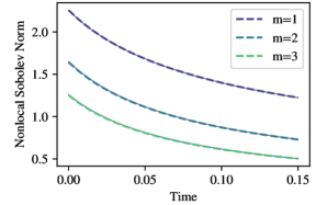
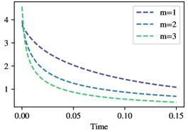
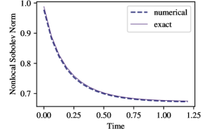
In Figure 3, we compute the evolution of the nonlocal Sobolev norm (49) along the numerical solutions from Figures 1 and 2. In both cases, we observe that the quantity converges as and decreases in time. This gives further credence to the heuristic that the nonlocal Sobolev norm is an approximation of the -norm of the gradient of the th power of the exact solution, which does decrease in time along the exact solution; see (24) and (25). In particular, this provides numerical evidence that Assumption (A1) from our main convergence theorem, Theorem 5.8, is satisfied.
Convergence Analysis: One-Dimensional Diffusion
Convergence Analysis: Two-Dimensional Diffusion
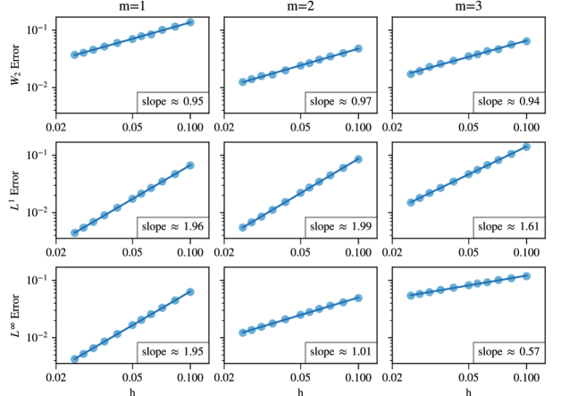
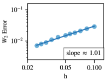
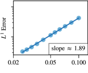
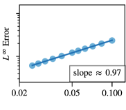
In Figure 4, we analyze the rate of convergence of our numerical scheme in one dimension. We compute the error between numerical and exact solutions of the heat and porous medium equations () in Figure 1 at time , with respect to the -Wasserstein distance, -norm, and -norm and examine the scaling of the error with the grid spacing . (Recall that throughout.) Plotting the errors on a logarithmic scale, we observe that the Wasserstein error depends linearly on the grid spacing for all values of . The -norm scales quadratically for and and superlinearly for . Finally, the -error scales quadratically for , superlinearly for , and sublinearly for . This deterioration of the rate of -convergence for is due to the sharp transition at the boundary of the exact solution; see the second row of Figure 1. In Figure 5, we perform the same analysis on the rate of convergence of our method in two dimensions and observe similar rates of convergence as in the one-dimensional case.
Fokker–Planck: Two Dimensions
Rate of Convergence to Steady State
Evolution of Density: Barenblatt and double bump initial data
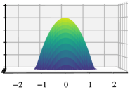
t = 0.0 t = 0.6 t = 1.2
t = 0.0 t = 0.6 t = 1.2
Evolution of Nonlocal Sobolev Norm: Barenblatt and double bump initial data
Barenblatt initial data Double bump initial data
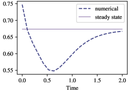
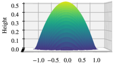
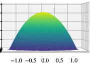
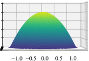
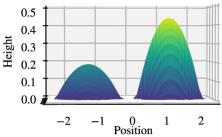
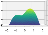
In Figure 6, we simulate solutions to the nonlinear Fokker–Planck equation (, , ) and consider the rate of convergence to the steady state of the equation, . In the top row, we compute the error between the numerical solution at time and the steady state with respect to the Wasserstein, -, and -norms for various choices of grid spacing . We consider solutions with Barenblatt initial data (, ). We plot the error’s dependence on with a logarithmic scale and compute the slope of the line of best fit to determine the scaling relationship between the error and . We observe similar rates of convergence as in the case of the heat and porous medium equations; see Figure 5. In the middle rows, we give snapshots of the evolution of the blob method solution, as it converges to the steady state. We consider Barenblatt initial data (, ) and double bump initial data given by a linear combination of Barenblatts, . The grid spacing is . In the bottom row, we compute the evolution of the nonlocal Sobolev norm (49) along the numerical solutions from the middle rows. In both cases, we observe that this quantity converges for small. For Barenblatt initial data, it decreases in time along the numerical solution and agrees well with the value of along the exact solution . For the double bump initial data, it remains bounded in time, converging asymptotically to , where is the steady state. Again, this supports the interpretation of the nonlocal Sobolev norm as an approximation of the -norm of the gradient of the th power of the exact solution and provides numerical evidence for Assumption (A1) from Theorem 5.8.
In the remaining numerical examples, we apply our method to simulate solutions of Keller–Segel type equations, with the interaction potential given by for . In one dimension, the derivative of this potential is not integrable, and we remove its singularity it setting it equal to for all such that . In two dimensions, the gradient of this potential is integrable, and we regularize it by convolving it with a mollifier , as done in previous work by the second author on a blob method for the aggregation equation [37].
One-Dimensional Keller–Segel Equation: Blow-up
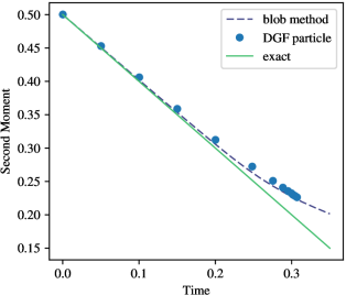
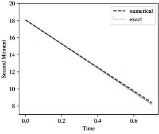
Evolution of Second Moment Evolution of Particle Trajectories
One-Dimensional Nonlinear Keller–Segel Equation: Convergence to Steady State
Evolution of Second Moment Evolution of Particle Trajectories
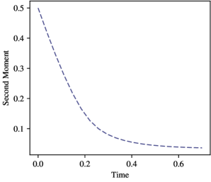
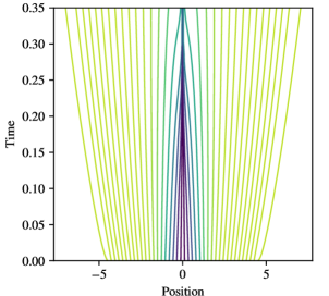
In Figure 7, we consider the one-dimensional variant of the Keller–Segel equation (, , ) studied in [19]. Its interest is that it has a defined critical value for unit mass leading to the dichotomy of blow-up versus global existence. For and initial data of mass one, solutions blow up in finite time. We consider initial data given by a Gaussian , , discretized on the interval with grid spacing . We compare the evolution of the second moment of our blob method solutions with the second moment of the exact solution. We also compare our results with those obtained in previous work via a one-dimensional Discrete Gradient Flow (DGF) particle method [31, 26]. By refining our spatial grid with respect to the DGF particle method, we observe modest improvements. (Alternative simulations, with similar spatial and time discretizations as used in the DGF method, yielded similar results as obtained by DGF.) The blow-up of solution is not only evident in the second moment, which converges to zero linearly in time, but also in the evolution of the particle trajectories. In particular, we observe particle trajectories merging on several occasions as time advances.
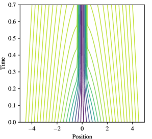
In Figure 8, we consider a nonlinear variant of the Keller–Segel equation (, , ) in one dimension, with initial data and discretization as in Figure 7. We observe the convergence to a steady state both at the level of the second moment and the particle trajectories.
Two-Dimensional Keller–Segel Equation: Evolution of Density
t = 0.0 t = 0.075 t = 0.15
Subcritical Mass
Critical Mass
Supercritical Mass
Two-Dimensional Keller–Segel Equation: Analysis of Blowup Behavior
Evolution of Second Moment, Convergence of Second Moment
Two-Dimensional Keller–Segel Equation: Blowup with Supercritical Mass
Evolution of Second Moment Evolution of Particle Trajectories
Two-Dimensional Keller–Segel Equation: Evolution of Density
t = 0.0 t = 0.075 t = 0.15
Subcritical Mass =
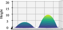
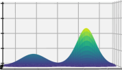
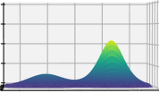
Critical Mass =
Supercritical Mass =
Evolution of Second Moment
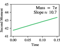
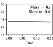
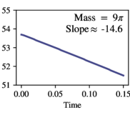
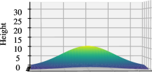
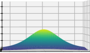
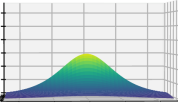
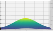
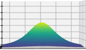
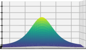
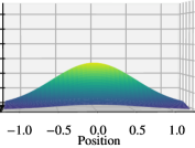
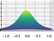
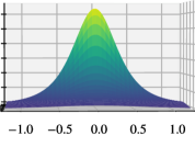
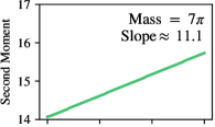
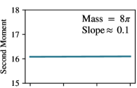
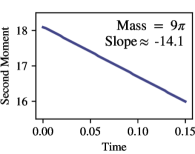
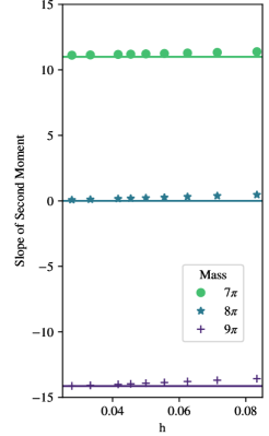
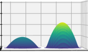
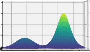
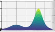
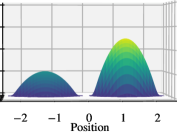
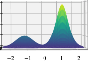
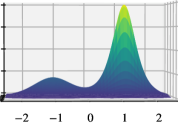
In Figures 9–12 we consider the classical Keller–Segel equation (, , ) in two dimensions. In Figures 9, 10, and 11, the initial data is given by a Gaussian , , scaled to have mass that is either supercritical (), critical (), or subcritical () with respect to blowup behavior. In particular, for supercritical initial data, solutions blow up in finite time [42, 14]. In Figure 9, we analyze the blow-up behavior. We compute the evolution of the second moment of solutions for fixed grid spacing and varying mass and , illustrating how initial data with larger mass aggregates more quickly at the origin.
In Figure 10, we consider the evolution of the second moment for the solutions from Figure 9. For fixed grid spacing , we observe that the second moment depends linearly on time, and we compute its slope using the line of best fit. We then analyze how the slope of this line converges to the theoretically predicted slope as the grid spacing .
In Figure 11, we consider the evolution of the second moment for the supercritical mass solution from Figure 9 on a longer time interval. As in the one-dimensional case (see Figure 7), we are able to get approximately halfway to the time when the second moment becomes zero before the second moment of our numerical solution begins to peel away from the second moment of the exact solution. Indeed, one of the benefits of our blob method approach is that the numerical method naturally extends to two and more dimensions, and we observe similar numerical performance independent of the dimension. We also plot the evolution of particle trajectories, observing the tendency of trajectories in regions of larger mass to be driven largely by pairwise attraction, while trajectories in regions of lower mass feel more strongly the effects of diffusion.
Appendix A Proofs of preliminary results
We now turn to the proofs of some of the elementary lemmas and propositions from Sections 2 and 3. We begin with the proof of the mollifier exchange lemma.
Proof of Lemma 2.2.
By the Lipschitz continuity of ,
Set . Decomposing the domain of the integration of into and , we may bound the above quantity by
By the decay assumption on (see Assumption 2.1), for all with we have
| (52) |
Thus, we conclude our result by estimating the above quantity by
We now give the proof that if , then .
Proof of Lemma 2.3.
By [3, Remark 5.1.6], it suffices to show that converges to in distribution, that is, in the duality with smooth, compactly supported functions. For all ,
Since , the second term goes to zero. We bound the first term as follows:
which goes to zero as . ∎
Next, we prove the inequalities relating the regularized internal energies to the unregularized internal energies.
Proof of Proposition 3.8.
We begin with (11). To prove the left inequality, we may assume without loss of generality that . First, we show the result for the entropy (). Note that
where is the relative entropy; that is, for all ,
By Jensen’s inequality for the convex function , the relative entropy is nonnegative, which gives the result. Now, we show the left inequality in (11) for . By the above-the-tangent property of the concave function and Hölder’s inequality, we get
Since implies , the first term goes to zero as and the second term remains bounded. This gives the result.
We now turn to the right inequality in (11) in the case . By the fact that and Jensen’s inequality for the concave function , for all we have
Consequently, we deduce
Now, we show (12). Since is convex for , this is simply a consequence of reversing the inequalities in the last two inequalities.
We now give the proof that, for all , the regularized energies are lower semicontinuous with respect to weak-* convergence () and Wasserstein convergence (), where in the latter case, we require to be a Gaussian.
Proof of Proposition 3.9.
First, we note that for any sequence and such that and any sequence , we have
| (53) | |||
since .
We now show (i). Suppose . By Lemma B.3, we have
By inequality (53),
Combining the two previous inequalities, we obtain , giving the result.
Next, we show (ii). Suppose in the Wasserstein metric. Since is a Gaussian, there exist and so that, for sufficiently large,
| (54) |
Define and . Then, by Lemma B.3, we have
| (55) |
Since in the Wasserstein metric,
| (56) |
Furthermore, by (53) and the fact that is continuous on ,
| (57) |
Thus, combining (55), (56), and (57), we obtain,
which gives the result. ∎
Now we turn to the proof that the regularized energies are differentiable along generalized geodesics.
Proof of Proposition 3.10.
By definition, for all ,
Therefore, we deduce
where . Using Taylor’s theorem compute
where is a term depending on the Hessian of satisfying
Hence, since is nondecreasing,
where . Note that converges pointwise to as since
Thus, to complete the result, it suffices to show that there exists so that
since the result then follows by the dominated convergence theorem. Since is nondecreasing we may take
which ends the proof. ∎
Next, we apply the result of the previous proof to characterize the subdifferential of the regularized energies.
Proof of Proposition 3.12.
Suppose is given by equation (16). This part of the proof is closely inspired by that of [25, Proposition 2.2]. For all define for all , where , with some , connects and . Now define
where ; see (15). We write for any . Let us compute the first two derivatives of for all :
| (58) |
and
Since , and is finite, we have
| (59) |
Now, by Taylor’s theorem,
and therefore, using (59) leads to
which shows that is nondecreasing, and so , which implies (after integrating against )
Then, by (58) and antisymmetry of , compute
Hence
which shows that . We now prove that . Consider a vector-valued function , and for any define for all . Then
Now compute, using the antisymmetry of ,
where passing the limit inside the integral in the first line is justified by the fact that is bounded. Then, by the definition of the local slope of ,
Therefore, by the previous computation,
since, by definition of the 2-Wasserstein distance,
Then, by replacing with , by arbitrariness of and by density of in , we get
which shows the desired result. Since is the unique minimal norm element of , this also shows that we actually have equality in the right-hand side above.
Suppose now that . Fix and define and for all . For sufficiently small, is convex and is the optimal transport map from to , so . Similarly, . Since , taking in Definition 2.7 of the subdifferential, for sufficiently small, gives
and
Combining this with Proposition 3.10, we obtain
Rewriting the expression from equation (14) gives
Thus, for , we have , i.e. in the sense of distribution. By [3, Proposition 8.4.3], since we get . Since we have already shown that the vector in (16) is the element of minimal norm of , we get that , and so . Again using [3, Proposition 8.4.3], we obtain , which ends the proof. ∎
Finally, we prove the characterization of the subdifferential of the full regularized energies .
Proof of Corollary 3.13.
Appendix B Weak convergence of measures
In this appendix, we recall several fundamental results on the weak convergence of measures. We begin with a result due to Ambrosio, Gigli, and Savaré on convergence of maps with respect to varying probability measures. This plays a key role in our proofs of both the -convergence of the energies and the convergence of the gradient flows.
DEFINITION B.1 (weak convergence with varying measures; c.f. [3, Definition 5.4.3]).
Given a sequence converging in the weak-∗ topology to some , we say that a sequence with for all converges weakly to some if
Furthermore, we say that converges strongly to in , , if
PROPOSITION B.2 (properties of convergence with varying measures; c.f. [3, Theorem 5.4.4]).
Let , and be such that for all . Suppose and for some . The following items hold.
-
(i)
There exists a subsequence of converging weakly to some .
-
(ii)
If weakly converges to some , then
-
(iii)
If strongly converges in to some and , then
We close by recalling a generalization of Fatou’s lemma, for varying measures.
LEMMA B.3 (Fatou’s lemma for varying measures; see, e.g., [46, Theorem 1.1], [4, Lemma 3.3]).
Consisder a sequence and so that . Then for any sequence of nonnegative functions on , we have
Acknowledgments: The authors thank Andrew Bernoff, Andrea Bertozzi, Eric Carlen, Yanghong Huang, Inwon Kim, Dejan Slepčev, and Fangbo Zhang for many helpful discussions.
References
- [1] M. Agueh. Local existence of weak solutions to kinetic models of granular media. Arch. Ration. Mech. Anal., 221(2):917–959, 2016.
- [2] L. Ambrosio and N. Gigli. A user’s guide to optimal transport. In Modelling and Optimisation of Flows on Networks, volume 2062 of Lecture Notes in Math., pages 1–155. Springer, Heidelberg, 2013.
- [3] L. Ambrosio, N. Gigli, and G. Savaré. Gradient Flows in Metric Spaces and in the Space of Probability Measures. Lectures in Mathematics ETH Zürich. Birkhäuser Verlag, Basel, 2008.
- [4] L. Ambrosio, N. Gigli, G. Savaré, et al. Bakry–émery curvature-dimension condition and riemannian ricci curvature bounds. The Annals of Probability, 43(1):339–404, 2015.
- [5] L. Ambrosio and G. Savaré. Gradient flows of probability measures. In Handbook of Differential Equations: Evolutionary Equations, volume 3 of Handb. Differ. Equ., pages 1–136. North-Holland, Amsterdam, 2007.
- [6] L. Ambrosio and S. Serfaty. A gradient flow approach to an evolution problem arising in superconductivity. Comm. Pure Appl. Math., 61(11):1495–1539, 2008.
- [7] C. Anderson and C. Greengard. On vortex methods. SIAM J. Numer. Anal., 22(3):413–440, 1985.
- [8] J.-D. Benamou, G. Carlier, Q. Mérigot, and E. Oudet. Discretization of functionals involving the Monge-Ampère operator. Numer. Math., 134(3):611–636, 2016.
- [9] M. Bessemoulin-Chatard and F. Filbet. A finite volume scheme for nonlinear degenerate parabolic equations. SIAM J. Sci. Comput., 34(5):B559–B583, 2012.
- [10] A. Blanchet, V. Calvez, and J. A. Carrillo. Convergence of the mass-transport steepest descent scheme for the sub-critical Patlak-Keller–Segel model. SIAM J. Numer. Anal., 46(2):691–721, 2008.
- [11] A. Blanchet, V. Calvez, and J. A. Carrillo. Convergence of the mass-transport steepest descent scheme for the subcritical Patlak–Keller–Segel model. SIAM J. Numer. Anal., 46(2):691–721, 2008.
- [12] A. Blanchet, E. A. Carlen, and J. A. Carrillo. Functional inequalities, thick tails and asymptotics for the critical mass Patlak-Keller–Segel model. J. Funct. Anal., 262(5):2142–2230, 2012.
- [13] A. Blanchet, J. Dolbeault, and B. Perthame. Two-dimensional Keller–Segel model: optimal critical mass and qualitative properties of the solutions. Electron. J. Differential Equations, (44), 2006.
- [14] A. Blanchet, J. Dolbeault, and B. t. Perthame. Two-dimensional Keller–Segel model: optimal critical mass and qualitative properties of the solutions. Electron. J. Differential Equations, pages No. 44, 32, 2006.
- [15] N. Bonneel, M. van de Panne, S. Paris, and W. Heidrich. Displacement interpolation using Lagrangian mass transport. ACM Trans. Graph., 30(6):158:1–158:12, 2011.
- [16] P. N. Brown, A. C. Hindmarsh, and G. D. Byrne. DVODE: Variable-coefficient Ordinary Differential Equation solver. Available at http://www.netlib.org/ode/vode.f.
- [17] M. Burger, J. A. Carrillo, and M.-T. Wolfram. A mixed finite element method for nonlinear diffusion equations. Kinet. Relat. Models, 3(1):59–83, 2010.
- [18] V. Calvez and T. O. Gallouët. Particle approximation of the one dimensional Keller–Segel equation, stability and rigidity of the blow-up. Discrete Contin. Dyn. Syst. Ser. A, 36(3):1175–1208, 2015.
- [19] V. Calvez, B. Perthame, and M. Sharifi tabar. Modified Keller–Segel system and critical mass for the log interaction kernel. In Stochastic analysis and partial differential equations, volume 429 of Contemp. Math., pages 45–62. Amer. Math. Soc., Providence, RI, 2007.
- [20] M. Campos-Pinto, J. A. Carrillo, F. Charles, and Y.-P. Choi. Convergence of a linearly transformed particle method for aggregation equations. Preprint, 2015.
- [21] E. A. Carlen and W. Gangbo. Solution of a model Boltzmann equation via steepest descent in the 2-Wasserstein metric. Arch. Ration. Mech. Anal., 172(1):21–64, 2004.
- [22] J. A. Carrillo, A. Chertock, and Y. Huang. A finite-volume method for nonlinear nonlocal equations with a gradient flow structure. Commun. Comput. Phys., 17(1):233–258, 2015.
- [23] J. A. Carrillo, Y.-P. Choi, and M. Hauray. The derivation of swarming models: mean-field limit and Wasserstein distances. In Collective Dynamics from Bacteria to Crowds: An Excursion Through Modeling, Analysis and Simulation, volume 553 of CISM Courses and Lect., pages 1–46. Springer Vienna, 2014.
- [24] J. A. Carrillo, K. Craig, L. Wang, and C. Wei. On primal dual splitting methods for nonlinear equations with a gradient flow structure. work in preparation.
- [25] J. A. Carrillo, M. Di Francesco, A. Figalli, T. Laurent, and D. Slepčev. Global-in-time weak measure solutions and finite-time aggregation for nonlocal interaction equations. Duke Math. J., 156(2):229–271, 2011.
- [26] J. A. Carrillo, Y. Huang, F. S. Patacchini, and G. Wolansky. Numerical study of a particle method for gradient flows. Kinet. Relat. Models, 10(3):613–641, 2017.
- [27] J. A. Carrillo, S. Lisini, and E. Mainini. Uniqueness for Keller–Segel-type chemotaxis models. Discrete Contin. Dyn. Syst., 34(4):1319–1338, 2014.
- [28] J. A. Carrillo, R. J. McCann, and C. Villani. Kinetic equilibration rates for granular media and related equations: entropy dissipation and mass transportation estimates. Rev. Mat. Iberoam., 19(3):971–1018, 2003.
- [29] J. A. Carrillo, R. J. McCann, and C. Villani. Contractions in the 2-Wasserstein length space and thermalization of granular media. Arch. Ration. Mech. Anal., 179(2):217–263, 2006.
- [30] J. A. Carrillo and J. S. Moll. Numerical simulation of diffusive and aggregation phenomena in nonlinear continuity equations by evolving diffeomorphisms. SIAM J. Sci. Comput., 31(6):4305–4329, 2009/10.
- [31] J. A. Carrillo, F. S. Patacchini, P. Sternberg, and G. Wolansky. Convergence of a particle method for diffusive gradient flows in one dimension. SIAM J. Math. Anal., 48(6):3708–3741, 2016.
- [32] J. A. Carrillo, H. Ranetbauer, and M.-T. Wolfram. Numerical simulation of nonlinear continuity equations by evolving diffeomorphisms. J. Comput. Phys., 327:186–202, 2016.
- [33] A. Chertock. A Practical Guide to Deterministic Particle Methods. Available at http://www4.ncsu.edu/~acherto/papers/Chertock_particles.pdf.
- [34] G.-H. Cottet and P. D. Koumoutsakos. Vortex methods. Cambridge University Press, Cambridge, 2000. Theory and practice.
- [35] G.-H. Cottet and P.-A. Raviart. Particle methods for the one-dimensional Vlasov–Poisson equations. SIAM J. Numer. Anal., 21(1):52–76, 1984.
- [36] K. Craig. Nonconvex gradient flow in the Wasserstein metric and applications to constrained nonlocal interactions. Proc. Lond. Math. Soc., 114(1):60–102, 2017.
- [37] K. Craig and A. L. Bertozzi. A blob method for the aggregation equation. Math. Comp., 85(300):1681–1717, 2016.
- [38] K. Craig and I. Topaloglu. Convergence of regularized nonlocal interaction energies. SIAM J. Math. Anal., 48(1):34–60, 2016.
- [39] P. Degond and S. Mas-Gallic. The weighted particle method for convection-diffusion equations. I. The case of an isotropic viscosity. Math. Comp., 53(188):485–507, 1989.
- [40] P. Degond and S. Mas-Gallic. The weighted particle method for convection-diffusion equations. II. The anisotropic case. Math. Comp., 53(188):509–525, 1989.
- [41] P. Degond and F.-J. Mustieles. A deterministic approximation of diffusion equations using particles. SIAM J. Sci. Statist. Comput., 11(2):293–310, 1990.
- [42] J. Dolbeault and B. t. Perthame. Optimal critical mass in the two-dimensional Keller–Segel model in . C. R. Math. Acad. Sci. Paris, 339(9):611–616, 2004.
- [43] B. Düring, D. Matthes, and J. P. Milišic. A gradient flow scheme for nonlinear fourth order equations. Discrete Contin. Dyn. Syst. Ser. B, 14(3):935–959, 2010.
- [44] L. Evans, O. Savin, and W. Gangbo. Diffeomorphisms and nonlinear heat flows. SIAM Journal on Mathematical Analysis, 37(3):737–751, 2005.
- [45] L. C. Evans. Partial Differential Equations, volume 19 of Graduate Studies in Mathematics. American Mathematical Society, Providence, RI, second edition, 2010.
- [46] E. A. Feinberg, P. O. Kasyanov, and N. V. Zadoianchuk. Fatou’s lemma for weakly converging probabilities. Theory of Probability & Its Applications, 58(4):683–689, 2014.
- [47] J. Goodman, T. Y. Hou, and J. Lowengrub. Convergence of the point vortex method for the -D Euler equations. Comm. Pure Appl. Math., 43(3):415–430, 1990.
- [48] L. Gosse and G. Toscani. Identification of asymptotic decay to self-similarity for one-dimensional filtration equations. SIAM J. Numer. Anal., 43(6):2590–2606, 2006.
- [49] L. Gosse and G. Toscani. Lagrangian numerical approximations to one-dimensional convolution-diffusion equations. SIAM J. Sci. Comput., 28(4):1203–1227, 2006.
- [50] M. Hauray. Wasserstein distances for vortices approximation of Euler-type equations. Math. Models Methods Appl. Sci., 19(8):1357–1384, 2009.
- [51] H. Huang and J.-G. Liu. Error estimate of a random particle blob method for the Keller–Segel equation. Math. Comp., 86(308):2719–2744.
- [52] J. D. Hunter. Matplotlib: a 2d graphics environment. Comput. Sci. Eng., 9(3):90–95, 2007.
- [53] P.-E. Jabin. A review of the mean field limits for Vlasov equations. Kinet. Relat. Models, 7(4):661–711, 2014.
- [54] P.-E. Jabin and Z. Wang. Mean field limit for stochastic particle systems. In Active Particles. Vol. 1. Advances in Theory, Models, and Applications, Model. Simul. Sci. Eng. Technol., pages 379–402. Birkhäuser/Springer, Cham, 2017.
- [55] E. Jones, T. Oliphant, P. Peterson, et al. SciPy: Open source scientific tools for Python, 2001–. Available at http://www.scipy.org/.
- [56] R. Jordan, D. Kinderlehrer, and F. Otto. The variational formulation of the Fokker–Planck equation. SIAM J. Math. Anal., 29(1):1–17, 1998.
- [57] O. Junge, D. Matthes, and H. Osberger. A fully discrete variational scheme for solving nonlinear Fokker–Planck equations in multiple space dimensions. SIAM J. Numer. Anal., 55(1):419–443, 2017.
- [58] A. Klar and S. Tiwari. A multiscale meshfree method for macroscopic approximations of interacting particle systems. Multiscale Model. Simul., 12(3):1167–1192, 2014.
- [59] G. Lacombe and S. Mas-Gallic. Presentation and analysis of a diffusion-velocity method. In Flows and Related Numerical Methods (Toulouse, 1998), volume 7 of ESAIM Proc., pages 225–233. Soc. Math. Appl. Indust., Paris, 1999.
- [60] A. J. Leverentz, C. M. Topaz, and A. J. Bernoff. Asymptotic dynamics of attractive-repulsive swarms. SIAM J. Appl. Dyn. Syst., 8(3):880–908, 2009.
- [61] P.-L. Lions and S. Mas-Gallic. Une méthode particulaire déterministe pour des équations diffusives non linéaires. C. R. Acad. Sci. Paris Sér. I Math., 332(4):369–376, 2001.
- [62] J.-g. Liu, L. Wang, and Z. Zhou. Positivity-preserving and asymptotic preserving method for 2d Keller–Segel equations. Accepted to Math. of Comp.
- [63] J.-G. Liu and R. Yang. A random particle blob method for the Keller–Segel equation and convergence analysis. Math. Comp., 86(304):725–745, 2017.
- [64] S. Mas-Gallic. The diffusion velocity method: a deterministic way of moving the nodes for solving diffusion equations. Transp. Theory and Stat. Phys., 31(4-6):595–605, 2002.
- [65] D. Matthes, R. J. McCann, and G. Savaré. A family of nonlinear fourth order equations of gradient flow type. Comm. Partial Differential Equations, 34(10-12):1352–1397, 2009.
- [66] R. J. McCann. A convexity principle for interacting gases. Adv. Math., 128(1):153–179, 1997.
- [67] K. Oelschläger. Large systems of interacting particles and the porous medium equation. Journal of differential equations, 88(2):294–346, 1990.
- [68] H. Osberger and D. Matthes. Convergence of a variational Lagrangian scheme for a nonlinear drift diffusion equation. ESAIM Math. Model. Numer. Anal., 48(3):697–726, 2014.
- [69] H. Osberger and D. Matthes. Convergence of a fully discrete variational scheme for a thin-film equation. Accepted at Radon Ser. Comput. Appl. Math., 2015.
- [70] H. Osberger and D. Matthes. A convergent Lagrangian discretization for a nonlinear fourth order equation. Found. Comput. Math., pages 1–54, 2015.
- [71] F. Otto. The geometry of dissipative evolution equations: the porous medium equation. Comm. Partial Differential Equations, 26(1-2):101–174, 2001.
- [72] F. S. Patacchini. A Variational and Numerical Study of Aggregation-Diffusion Gradient Flows. PhD thesis, Imperial College London, 2017.
- [73] R. Piessens, E. de Doncker-Kapenga, C. W. Überhuber, and D. K. Kahaner. QUADPACK: a Subroutine Package for Automatic Integration, volume 1 of Computational Mathematics. Springer-Verlag, Berlin Heidelberg, 1983.
- [74] F. Riesz and B. Sz.-Nagy. Functional Analysis. Dover Books on Advanced Mathematics. Dover Publications, Inc., New York, 1990.
- [75] G. Russo. Deterministic diffusion of particles. Comm. Pure Appl. Math., 43(6):697–733, 1990.
- [76] G. Russo. A particle method for collisional kinetic equations. i. basic theory and one-dimensional results. J. Comput. Phys., 87(2):270–300, 1990.
- [77] E. Sandier and S. Serfaty. Gamma-convergence of gradient flows with applications to Ginzburg–Landau. Comm. Pure Appl. Math., 57(12):1627–1672, 2004.
- [78] F. Santambrogio. Optimal Transport for Applied Mathematicians: Calculus of Variations, PDEs, and Modeling, volume 87 of Progress in Nonlinear Differential Equations and their Applications. Birkhäuser/Springer, Cham, 2015.
- [79] S. Serfaty. Gamma-convergence of gradient flows on Hilbert and metric spaces and applications. Discrete Contin. Dyn. Syst., 31(4):1427–1451, 2011.
- [80] R. Simione, D. Slepčev, and I. Topaloglu. Existence of ground states of nonlocal-interaction energies. J. Stat. Phys., 159(4):972–986, 2015.
- [81] Z. Sun, J. A. Carrillo, and C.-W. Shu. A discontinuous Galerkin method for nonlinear parabolic equations and gradient flow problems with interaction potentials, preprint. Preprint, 2017.
- [82] S. van der Walt, C. Colbert, and G. Varoquaux. The numpy array: a structure for efficient numerical computation. Comput. Sci. Eng., 13(2):22–30, 2011.
- [83] C. Villani. Topics in optimal transportation, volume 58 of Graduate Studies in Mathematics. American Mathematical Society, Providence, RI, 2003.
- [84] C. Villani. Optimal Transport: Old and New, volume 338 of Grundlehren der Mathematischen Wissenschaften. Springer-Verlag, Berlin, 2009.
- [85] M. Westdickenberg and J. Wilkening. Variational particle schemes for the porous medium equation and for the system of isentropic Euler equations. M2AN Math. Model. Numer. Anal., 44(1):133–166, 2010.