Searching for the full symphony of black hole binary mergers

Abstract

Current searches for the gravitational-wave signature of compact binary mergers rely on matched-filtering data from interferometric observatories with sets of modelled gravitational waveforms. These searches currently use model waveforms that do not include the higher-order mode content of the gravitational-wave signal. Higher-order modes are important for many compact binary mergers and their omission reduces the sensitivity to such sources. In this work we explore the sensitivity loss incurred from omitting higher-order modes. We present a new method for searching for compact binary mergers using waveforms that include higher-order mode effects, and evaluate the sensitivity increase that using our new method would allow. We find that, when evaluating sensitivity at a constant rate-of-false alarm, and when including the fact that signal-consistency tests can reject some signals that include higher-order mode content, we observe a sensitivity increase of up to a factor of 2 in volume for high mass ratio, high total-mass systems. For systems with equal mass, or with total mass $\sim 50M_{\odot}$, we see more modest sensitivity increases, $<10\%$, which indicates that the existing search is already performing well. Our new search method is also directly applicable in searches for generic compact binaries.

I Introduction

The Advanced LIGO gravitational-wave observatories Aasi et al. (2015a) have observed multiple black hole binary mergers in Advanced LIGO’s first two observing runs Abbott et al. (2016a, b, 2017a). Many additional black hole binary mergers are expected to be observed in the coming years Abbott et al. (2017a), with additional detectors in Italy Acernese et al. (2015), Japan Aso et al. (2013) and India Iyer et al. (2011) helping to improve coverage of the gravitational-wave sky Abbott et al. (2016c). The continued observation of black hole binary mergers will allow for a better understanding of the rate of such mergers Abbott et al. (2016d), and give a sense of the mass and component spin distribution of black hole binary systems Abbott et al. (2016e, f). This will in turn allow a better understanding of how such systems form Amaro-Seoane and Santamaria (2010); Amaro-Seoane (2012); Gair et al. (2011); Sesana et al. (2009); Volonteri (2012a, b).

Searches for compact binary mergers rely on matched filtering the data taken from gravitational-wave observatories with theoretical filter waveforms Nitz et al. (2017a); Usman et al. (2015); Dal Canton et al. (2014); Cannon et al. (2012, 2013). The set of filter waveforms is chosen such that a signal occurring anywhere within the parameter space of interest can be recovered well by at least one of the waveforms in the set of filters Sathyaprakash and Dhurandhar (1991); Babak et al. (2006); Ajith et al. (2014); Brown et al. (2012); Capano et al. (2016). It is critical that the waveform models being used as filters are accurate representations of the signals that will be produced from compact binary mergers in the Universe. Much work in the years leading up to Advanced LIGO’s first discovery focused on modelling waveforms using numerical Pretorius (2005); Szilagyi et al. (2009); Scheel et al. (2009); Frauendiener (2011); Hannam et al. (2010); Chu (2011); Vaishnav et al. (2007); Herrmann et al. (2007); Healy et al. (2009) and analytical Blanchet et al. (1995); Buonanno and Damour (1999) techniques, and on combining these methods together to create waveform models accurate at all stages of the merger Taracchini et al. (2012); Bohé et al. (2017); Ajith et al. (2008); Khan et al. (2016) .

However, a number of assumptions are made about the emitted gravitational-wave signal to simplify the search and reduce the search parameter space. Specifically, current searches for compact binary mergers neglect any affect due to precession of the orbital plane Apostolatos et al. (1994), orbital eccentricity Damour et al. (2004) or neutron-star equation-of-state Flanagan and Hinderer (2008); Read et al. (2013). Current searches also neglect the affect of the so-called higher-order modes of gravitational-wave emission Blanchet et al. (2008), and it is on this topic that we will focus in this manuscript. Making these simplifying assumptions does not affect the ability to observe the majority of compact binary mergers, as evident from the current observations, but can mean that the detection efficiency is not optimal. It would also induce an observational bias against compact binary mergers that are not well described by these assumptions, and these kind of systems can be the ones of most value, astrophysically, as the additional information from features such as higher-order modes allows more precise measurement of the various source parameters O’Shaughnessy et al. (2014).

Several studies have shown that the omission of higher-order modes in searches can lead to a reduction in detection rate McKechan (2011); Pekowsky et al. (2013); Capano et al. (2014); Varma et al. (2014); Calderón Bustillo et al. (2016, 2017). Specifically, the omission of higher modes is likely to reduce the detection of systems with large mass ratio $q=m_{1}/m_{2}\geq 4$ and large total mass $M=m_{1}+m_{2}>100M_{\odot}$ Pekowsky et al. (2013); Capano et al. (2014); Varma et al. (2014); Calderón Bustillo et al. (2016, 2017). To date Advanced LIGO has only detected systems with mass ratios and total masses lower than these values. However, we still know very little about the mass distribution of compact binary mergers and searches should be capable of observing any possible system. For such high-mass systems, more loosely modelled search techniques Klimenko et al. (2008); Sutton et al. (2010); Cornish and Littenberg (2015); Lynch et al. (2017); Klimenko et al. (2016) also offer the ability to observe short duration compact binary mergers Mazzolo et al. (2014). For very high-mass systems the sensitivity of such searches can become comparable to that of modelled search methods, and could potentially exceed the sensitivity of modelled searches in the case that the system is not well described by the model. Nevertheless, in cases where the waveform model is well understood, searches that use that knowledge should be more sensitive than those that don’t.

In this study, we present the first end-to-end modelled search method for black hole binary mergers using filter waveforms that include the higher-order modes of the gravitational-wave signals and demonstrate the improvement in sensitivity that can be obtained when using this method to search for compact binary mergers in Advanced LIGO data. Our method involves including the source orientation angles in the list of parameters that are sampled over when creating a set of filter waveforms to use in the search. At the time of writing, the only waveform model that is available including both the full inspiral, merger and ringdown components of the waveform and including higher-order modes, is the non-spinning effective-one-body model presented in Pan et al. (2011). We must therefore restrict ourselves in this work to only considering waveforms that do not include the effects of the components’ spins. However, the methods we describe here are directly applicable to the case of aligned-spin waveform models, which are now in an advanced stage of development London et al. (2017); Cotesta et al. (2017). Indeed the search method presented here is fully generic, and could be run on eccentric, precessing waveforms including higher-order modes.

The layout of this paper is as follows. In section II we motivate the parameter range that we choose to consider in this work. In section III we give a brief reminder of how the presence of higher-order modes will affect the emitted gravitational-wave signal, and discuss the waveform models used in this work. In section IV we introduce the fully generic search method that we will use. In section V we assess the benefit of deploying a search including the higher-order mode components of the gravitational-wave signal. In section VI we also explore how signal-based consistency tests, necessary in searches of real data to distinguish real signals from instrumental transients, can sometimes falsely reject real gravitational-wave signals containing higher-order modes, and how this problem is alleviated when using higher-order mode waveforms as filters. Finally we conclude in section VII.

II Parameter space considerations

In this section we motivate and describe the black hole binary parameter space that we will use in the rest of this work. While we will use a specific parameter space here, we stress again that the search methods we will describe can be applied for any parameter space of interest.

It was recently reported that no gravitational-wave signals were observed in a search of Advanced LIGO data targeting “intermediate mass black hole binaries”, which are defined to be black hole binaries with total mass $M\geq 100M_{\odot}$ Abbott et al. (2016e).

These sources are important from an astrophysical point of view. They are proposed to be precursors of supermassive black holes in some hierarchical formation scenarios Amaro-Seoane and Santamaria (2010); Amaro-Seoane (2012); Gair et al. (2011); Sesana et al. (2009); Volonteri (2012a, b). However, there is not yet evidence for their existence. Detection of higher-order modes would allow for more detailed tests of General Relativity in the strong field regime. Examples of this include studies of the quasi-normal ringdown modes Gossan et al. (2012); Yang et al. (2017) and studies evaluating the mass of the graviton via searching for a dispersion relation in the speed of propagation of gravitational-waves Berti et al. (2015). For the kind of sources considered in that work, higher-modes are believed to have a significant impact on gravitational-wave signals Pekowsky et al. (2013); Varma et al. (2014); Calderón Bustillo et al. (2016, 2017).

The effect of higher-order modes was not studied in the search for “intermediate mass black hole binaries” reported in Abbott et al. (2016e); both the waveforms used in the search, and the simulations to assess its sensitivity, did not include higher-order modes. It is therefore interesting to explore the same parameter space here and assess whether neglecting higher-order modes is a fair assumption in such studies, and to demonstrate the sensitivity increase that is possible if higher-order modes are included. The matched-filter search used in Abbott et al. (2016e) targeted black hole binary mergers with total mass between $50M_{\odot}$ and $600M_{\odot}$. At $600M_{\odot}$ compact binary mergers emit gravitational-wave signals that are for the most part too low frequency to be observed by Advanced LIGO and the sensitive distance rapidly decreases. It is also challenging to distinguish such signals from non-Gaussianities in the detector noise. Here we choose to use a maximum total mass of $400M_{\odot}$. Our constraints on the mass ratio, $q$, are limited by constraints on the waveform model we use, which we will discuss in the next section. We use a limit of $q\leq 10$, which also matches the limits chosen in Abbott et al. (2016e). When we discuss masses in this work we will always refer to the masses of the signal observed by the observatory, often referred to as “detector frame masses”. Sources at cosmological distances will be redshifted with respect to the observer, causing the signal to appear to have higher masses than the actual ones measured in the “source frame”.

The sensitivity of Advanced LIGO has been improving since the beginning of Advanced LIGO’s first observing run and will continue to improve over the next years, before reaching its design sensitivity. In order to obtain reasonable estimates of the improvements derived from our search method, we will use two noise curves in this study. We will use a representative measurement of the sensitivity curve from Advanced LIGO’s first observing run (O1) Sigg (2016) and we will use Advanced LIGO’s “zero-detuned high-power” design sensitivity curve Shoemaker (2015). For the former, we set the lower frequency of our matched-filter to $f_{low}=20$Hz while for the latter we use $f_{low}=10$Hz.

III Gravitational-wave signals including higher-order modes

The gravitational-wave emission from a non eccentric black hole binary merger depends on 15 parameters. The individual masses, $m_{i}$, and dimensionless angular momenta (spins), $\vec{\chi}_{i}=\vec{s}_{i}/m_{i}$, of its two components are parameters intrinsic to the source—collectively denoted $\Xi_{i}$. The time of the coalescence, measured in the frame of the observer, is denoted $t_{c}$. The remaining parameters describe the location and orientation of the observer, with respect to the source. Consider a frame of reference in standard spherical coordinates $(D,\iota,\varphi)$ with origin in the center of mass of the black hole binary. The polar angle $\iota$ is defined such that $\iota=0$ coincides with the total angular momentum of the binary. The remaining 3 parameters are the sky-location of the source in the frame of the observer $(\theta,\phi)$, and the polarisation $\psi$ of the signal. A black hole binary is said to be “face-on” if $\iota=0$ or $\iota=\pi$ and “edge-on” if $\iota=\pi/2$.

For a generic gravitational-wave source observed by an interferometric detector the observed strain $h(t)$ can be expressed as the sum of the two gravitational-wave polarizations weighted by the sensitivity of the observer to each polarization

$$h(t)=F_{+}(\theta,\phi,\psi)h_{+}(t)+F_{\times}(\theta,\phi,\psi)h_{\times}(t).$$ (1)

Here $F_{+}$ and $F_{\times}$ denote the response function of the detector to each polarization Finn and Chernoff (1993); Jaranowski et al. (1998). The gravitational-wave polarizations $h_{+}(t)$ and $h_{\times}(t)$ can be expressed as

$$h_{+}(t)+ih_{\times}(t)=\sum_{\ell\geq 2}\sum_{m=-\ell}^{m=\ell}Y^{-2}_{\ell,m}(\iota,\varphi)h_{\ell,m}(t),$$ (2)

where $Y^{-2}_{lm}$ denote the spherical harmonics of weight $-2$ Goldberg et al. (1967) and the $h_{\ell,m}(t)$ denote the various “modes” of gravitational-wave emission. For the case of compact binary mergers $h_{\ell,m}(t)$ will be a function of $\Xi_{i}$, $t_{c}$ and $D$ according to

$$h_{\ell,m}(\Xi;t)=A_{\ell,m}(\Xi,D;t-t_{c})e^{-i\upsilon_{\ell,m}(\Xi;t-t_{c})}.$$ (3)

Here $A_{\ell,m}$ is a real amplitude scaling for the various modes, and $\upsilon_{\ell,m}$ is a real time-series giving the evolution of the phase of the various modes.

The black hole binaries detected by LIGO so far are characterized by a low mass ratio $q\leq 4$ and a total mass $M<100M_{\odot}$ Abbott et al. (2016e, b, 2017a). For such sources the $(\ell,m)=(2,\pm 2)$ modes dominate the above sum for the vast majority of the possible orientations of the source Pekowsky et al. (2013). The rest of the modes, known as higher-order modes, have only a small contribution during most of the inspiral and are only significant to the resulting gravitational-wave signal in the last few cycles and eventual merger of the black hole binary Healy et al. (2013); Bustillo et al. (2015); Calderón Bustillo et al. (2016). The amplitude of the higher-order modes grows as the mass ratio $q$ of the system deviates from $1$, making their impact much stronger for large mass ratio black hole binaries. In addition, the $Y^{-2}_{2,\pm 2}$ spherical harmonics have maxima at $\iota=0$ and $\iota=\pi$ and a minimum at $\iota=\pi/2$. For many of the other harmonics $\iota=\pi/2$ is a maximum. Therefore, the $(\ell,m)=(2,\pm 2)$ modes will completely dominate the gravitational-wave signal for face-on sources. For edge-on systems, especially ones with a high-mass ratio, the higher-order modes are an important contribution to the full gravitational-wave emission McKechan (2011); Pekowsky et al. (2013); Capano et al. (2014); Varma et al. (2014); Calderón Bustillo et al. (2016, 2017). In addition, higher-order modes have a stronger affect in signals emitted by large total mass sources. The phase of the $(\ell,m)$ mode scales, to good accuracy, as $\upsilon_{\ell,m}\propto m\times\upsilon_{orb}/M$, where $\upsilon_{orb}$ denotes the orbital phase of the binary. At high values of total mass, $M$, the dominant $(2,\pm 2)$ modes can fall below the sensitive band of the observatory, while the higher $m$ modes, at higher frequency, are still observable.

Waveform models that describe the full black-hole binary coalescence—through inspiral, merger and ringdown—can be broadly divided into two approaches. The first is the “effective-one-body” approach, calibrated against numerical relativity simulations Buonanno and Damour (1999); Taracchini et al. (2012); Damour et al. (2013); Bohé et al. (2017), the second is the various phenomenological frameworks, also calibrated against numerical relativity simulations Santamaria et al. (2010); Hannam et al. (2014); Khan et al. (2016). There are a number of different waveform models, from both of these approaches, which have been used in the recent results papers from the LIGO and Virgo collaborations. However, with the exception of numerically generated waveforms, which are currently impractical to use for searches with a wide parameter space, these waveform models do not include the higher modes of the gravitational-wave emission, and consider solely the dominant modes. The only waveform model available at the time of this study, which includes both higher-order modes and includes the merger and ringdown components of the gravitational-wave signal is an effective-one-body waveform described in Pan et al. (2011). This model includes the $(\ell,|m|)=(2,\pm 1),(2,\pm 2),(3,\pm 3),(4,\pm 4)$ and $(5,\pm 5)$ modes. The most significant mode not included in this model is the $(3,\pm 2)$ mode, which can have comparable amplitude to the $(5,5)$ mode Pan et al. (2011); Healy et al. (2013). While the paper Pan et al. (2011) does demonstrate the accuracy of this model to generic waveforms, it would of course be beneficial to have this, and other modes, included in future waveform models. Unfortunately, this effective-one-body waveform model does not include the effect of the components’ spins. Nevertheless this non-spinning waveform model is sufficient to demonstrate the methodology described later in this work, and with it we can investigate the sensitivity increase to non-spinning compact binary mergers if one searches with waveform filters that include higher-order modes. We might expect that the relative sensitivity with non-spinning waveforms would be similar to that with aligned-spin waveforms as the effects of spin inclusion and higher-order modes are largely orthogonal. However, it is true that systems with anti-aligned spins have slightly stronger higher modes than systems with aligned spins Varma and Ajith (2016) and therefore it is possible that higher-modes would help more for negative spin sources than for positive ones. We will investigate this in the future when waveform models are available to do so.

Finally, we note that during the writing of this manuscript a number of waveform models, in both the effective-one-body and phenomenological frameworks are being developed that include higher-order modes, and allow for nonzero component spins aligned with the orbital angular momentum London et al. (2017); Cotesta et al. (2017). The methods described here can be applied directly to these waveform models when they become available, and this would be a necessary step before utilising this methodology to search for higher-order mode waveforms in real data. There is also work demonstrating that sets of numerical relativity waveform might be used directly in a search Kumar et al. (2014), or that surrogate models could be created by interpolating between a set of numerical relativity waveforms Szilagyi et al. (2015); Blackman et al. (2017a, b). Such approaches might also present a way to use accurate aligned-spin, or even precessing, higher-order mode waveforms in searches, but we do not explore that here.

IV A modelled search for compact binary mergers with higher-order mode waveforms

There are currently a number of different search methods being used to observe compact binary coalescences using modelled waveforms in the data being collected by Advanced LIGO and Advanced Virgo Cannon et al. (2012); Babak et al. (2013); Cannon et al. (2013); Dal Canton et al. (2014); Adams et al. (2016); Usman et al. (2015); Nitz et al. (2017a). The core of all of these different methods is the two-phase matched-filter that was described in Sathyaprakash and Dhurandhar (1991); Allen et al. (2012). This two-phase matched-filter has proved to be very powerful in observing compact binary mergers, but it does make a number of assumptions about the signal model, which are not true generically, in particular when one is considering higher-order modes. Specifically the method assumes that the normalized frequency domain representation of the $+$ component of the gravitational wave signal $\tilde{h}_{+}$ is related to the frequency domain representation of the $\times$ component of the gravitational wave signal $\tilde{h}_{\times}$ according to $\tilde{h}_{+}\propto i\tilde{h}_{\times}$. In addition, it is assumed that the “extrinsic” parameters of a gravitational-wave signal—the sky-location, source orientation, polarization phase and distance—can all be absorbed by applying a constant phase-shift, constant time-shift and a constant amplitude scaling to the observed waveform. With these assumptions in place, one can analytically maximize over an overall amplitude and phase of the signal, and use an inverse Fourier transform to quickly evaluate the statistic as a function of time Sathyaprakash and Dhurandhar (1991); Allen et al. (2012). Then only the “intrinsic” parameters—the component masses and spins—are searched over by repeating the search process with a well chosen discrete set of waveform models with varying values of the component masses and spins, known as the “template bank”. Physically, these assumptions hold if one assumes that the sources being observed have no orbital eccentricity, no precession and no contribution from higher-order modes to the gravitational-wave signal. However, these assumptions do not hold in the case here where we wish to use waveforms including higher-order modes as filters in the search.

In Pan et al. (2004); Harry et al. (2016) the authors explored relaxing the assumption that the system was not precessing and developed search statistics that can be used in that case. In the method described in Pan et al. (2004) a complex maximization scheme was used to maximize over all non-intrinsic parameters, which was found to be computationally prohibitive if forced to restrict to only physically possible values. Whereas, in Harry et al. (2016) the authors included the inclination of the source with respect to the observer as a parameter when constructing the template bank, effectively considering this as an intrinsic parameter. However, this method cannot be applied to a generic search because the assumption that the $\varphi$ parameter (the azimuthal angle to the observer in the source frame) can be modelled as an overall phase shift in the Fourier domain breaks down when considering gravitational-wave signals with higher-order modes.

Nevertheless one can extend the method in Harry et al. (2016) in a reasonably trivial manner by relaxing the assumption on $\varphi$ and also considering this as a parameter to search over in the template bank. This is the approach we use in this work. The resulting statistic is not new to this work, it also appears in Capano et al. (2014); Schmidt et al. (2015). This work, however, is the first case in which this has been applied in an end-to-end search.

IV.1 A search statistic applicable for generic searches for compact binary mergers

When searching for a signal $h$, with known form, but unknown amplitude, in Gaussian, stationary noise $n$, with noise-power spectral density $S_{n}(f)$ it can be demonstrated Maggiore (2007); Creighton and Anderson (2011) that the optimal statistic for deciding whether a signal $h$ is present, or not, in the data is given by

$$\rho^{2}\equiv\frac{\left(\operatorname{\mathbb{R}e}\left[\left\langle s|h\right\rangle\right]\right)^{2}}{\left\langle h|h\right\rangle}=\left(\operatorname{\mathbb{R}e}[\langle s|\hat{h}\rangle]\right)^{2},$$ (4)

where $\rho$ defines a signal-to-noise ratio, $\hat{a}$ denotes a normalization of any filter waveform $a$ such that

$$\hat{a}=\frac{a}{\left\langle a|a\right\rangle^{\frac{1}{2}}},$$ (5)

and we define the complex matched-filter

$$\langle a|b\rangle=4\int^{\infty}_{0}\frac{\tilde{a}(f)\tilde{b}^{*}(f)}{S_{n}(f)}df.$$ (6)

For simplicity in what follows, we will distinguish between the complex matched-filter, and the real component of the complex matched-filter by defining

$$\left(a|b\right)=\operatorname{\mathbb{R}e}\left[\langle a|b\rangle\right],$$ (7)

such that

$$\rho^{2}=\left(\operatorname{\mathbb{R}e}[\langle s|\hat{h}\rangle]\right)^{2}=(s|\hat{h})^{2}.$$ (8)

As already mentioned in section III, gravitational-wave signals observed in an interferometric observatory such as LIGO or Virgo can be expressed as a linear combination of the two gravitational-wave polarizations

$$h(t)=F_{+}(\theta,\phi,\psi)\,h_{+}(t)+F_{\times}(\theta,\phi,\psi)\,h_{\times}(t).$$ (9)

As the amplitude of $h(t)$ is removed by normalization in equation 8 we can freely scale the amplitude when defining $h(t)$. It is convenient to combine $F_{+}$ and $F_{\times}$ into an overall amplitude rescaling and a single further parameter by defining

$$h(t)=A(u\hat{h}_{+}(t)+\hat{h}_{\times}(t)),$$ (10)

where

$$u=\frac{F_{+}}{F_{\times}}\sqrt{\frac{\left\langle\hat{h}_{+}|\hat{h}_{+}\right\rangle}{\left\langle\hat{h}_{\times}|\hat{h}_{\times}\right\rangle}}$$ (11)

and

$$A=F_{\times}\sqrt{\left\langle\hat{h}_{\times}|\hat{h}_{\times}\right\rangle}.$$ (12)

One can then insert equation 10 into equation 8, which removes the amplitude term $A$, and from there analytically maximize $\rho$ over $u$. This results in the following expression,

$$\max_{u}(\rho^{2})=\frac{(s|\hat{h}_{+})^{2}+(s|\hat{h}_{\times})^{2}-2(s|\hat{h}_{+})(s|\hat{h}_{\times})(\hat{h}_{+}|\hat{h}_{\times})}{\left(1-(\hat{h}_{+}|\hat{h}_{\times})^{2}\right)}.$$ (13)

Furthermore it is trivial to see that in the limit that $\tilde{h}_{+}\propto i\tilde{h}_{\times}$ this will collapse to the more familiar statistic used in current searches

$$\max_{u}(\rho^{2})\simeq\left\|\left\langle s|\hat{h}_{+}\right\rangle\right\|^{2}.$$ (14)

The statistic defined in equation 13 is generic and can be applied to any single detector search for compact binary coalescences. Physically, this statistic maximizes over the $D$, $\theta$, $\phi$ and $\psi$ parameters—or the distance, sky location and polarization phase—leaving all other parameters to be included in the template bank. For the case of eccentric, precessing, higher-order mode waveforms, this will result in a very large dimension parameter space, which may prove unfeasible in some situations. In such cases approaches such as the ones explored in Pan et al. (2004); Dhurandhar et al. (2017) might be useable to further shrink the dimensionality of the parameter space by maximizing over the $Y^{-2}_{\ell,m}$ components, but this has yet to be successfully applied to generic systems. However, as we explore below, our simple approach can successfully be applied to the case of searching for higher-order mode signals in Advanced LIGO data.

IV.2 Exploring the necessity of the generic statistic for higher-order mode searches

In equation 13 we described a generic matched-filter statistic that maximizes only over the amplitude, polarization phase and sky location of the signal. While this statistic can be used generically, it is more computationally efficient to use the more commonly used statistic in equation 14 as it requires only one matched-filter computation. Equation 13 collapses to the form shown in 14 in the case when $\tilde{h}_{+}\propto i\tilde{h}_{\times}$. It is therefore worth investigating how well this relationship holds in the parameter space being considered to decide whether it is possible to approximate equation 13 with the more efficient equation 14. It is also possible to use the more efficient statistic in some part of the parameter space and swap over to the generic statistic only in the regions of parameter space where it is needed.

Figure 1: The imaginary component of the complex overlap between $\hat{h}_{+}$ and $\hat{h}_{\times}$ for the representative early Advanced LIGO noise curve (top), and for the predicted design sensitivity curve of Advanced LIGO (bottom). The overlap is numerically minimized over inclination and reference orbital phase within each of the pixels shown on these plots.

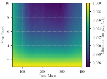
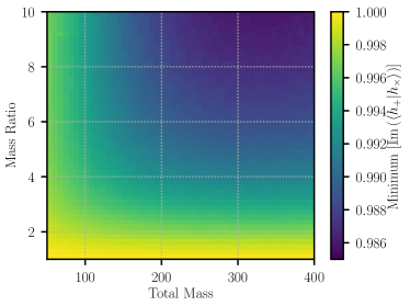
To investigate the possibility of using this approximation, we can simply calculate the magnitude of the imaginary component of the overlap between $\hat{h}_{+}$ and $\hat{h}_{\times}$ for systems within the parameter space defined in Section II. To do this we generate 5 million waveforms, with component masses uniformly chosen within our chosen parameter space, and with isotropic distribution of inclination and reference orbital phase. For each of these waveforms we compute the imaginary component of the overlap between $\hat{h}_{+}$ and $\hat{h}_{\times}$, $\operatorname{\mathbb{I}m}\left(\langle\hat{h}_{+}|\hat{h}_{\times}\rangle\right)$. The results are then binned in terms of the total mass and mass ratio, and we show the minimum value of this overlap, as a function of the total mass and mass ratio in figure 1. We see that for both the early and design Advanced LIGO sensitivity curves the minimum value of this overlap is $\sim 0.985$. If we were instead to plot the average value of this overlap the value would be larger than 0.997 everywhere. These values indicate the largest loss of signal-to-noise ratio that is possible when making the assumption that the polarization phase can be simplified. For example in the case where the value of the imaginary component of the overlap is 0.985, then $1.5\%$ of the maximum signal-to-noise ratio would be lost if the signal observed in the detector is described by the $\times$ component of $h(t)$ and the $+$ component is used as a template. For other values of polarization phase—such that the detector would observe a combination of the $+$ and $\times$ components—$>98.5\%$ of the optimal signal-to-noise ratio would be recovered. Given that we will allow a $3\%$ loss of signal-to-noise ratio due to the discreteness of the set of filter waveforms used, this indicates that for the parameter spaces and noise curves that we consider in this work it is sufficient to use the simple statistic in all regions of parameter space. We also verify this claim later in the results sections. We emphasize though that if this method is used in future searches using an extended region of parameter space, or including effects of spin precession, this should be evaluated again.

V Assessing the sensitivity increase of a higher-order mode search

In the previous section we described a method that will allow the use of template waveforms that include higher-order modes in searches for compact binary mergers. In this section we will assess the increase in sensitivity that can be obtained by using this method to search for compact binary mergers in Advanced LIGO data. We begin by creating “template banks” of waveforms to cover the full parameter space described earlier in section II. From there we will explore the sensitivity increase that can be obtained when using higher-order mode waveforms. We will first assess this by comparing sensitivities above a constant signal-to-noise ratio threshold, for both the standard search, and our new method using higher-order mode waveforms. We will also identify the points in parameter space for which the sensitivity increases the most when including higher-order mode waveforms. Finally, we will use our new method in the PyCBC analysis framework Dal Canton et al. (2014); Usman et al. (2015); Nitz et al. (2017b) to analyse 5 days of Gaussian noise, colored to Advanced LIGO sensitivities. This will allow us to assess the increase in the background rate when including the larger number of templates that are needed to cover the higher-order mode signal parameter space. This will then enable us to compute the sensitivity increase at a constant false-alarm rate threshold between a search that includes the effects of higher-order modes, and one that does not.

V.1 A template bank of filter waveforms including higher order modes

The first step in assessing the sensitivity improvement that can be achieved by including the effects of higher-order modes in the filter waveforms is to create the set of filter waveforms, or “template bank”. In this sub-section we describe the construction of the template banks that we will use, highlighting any problems specific to construction of template banks of higher-order mode signals.

Figure 2: The left panel shows the distribution of templates, as a function of the total mass and mass ratio, for the template bank created for the early Advanced LIGO noise curve. The black crosses indicate the templates that are needed to cover the parameter space if higher-order modes are omitted, the red circles indicate the additional templates that are required if higher-order modes are included in the search parameter space. The right panel shows the distribution of the inclination angle of the higher-order mode waveforms in the template bank created for the Advanced LIGO design noise curve.

We begin by defining the overlap, $o(a,b)$, between a potential signal waveform $a$ and a filter waveform $b$ as the fraction of the optimal signal-to-noise-ratio $(a|a)$ of $a$ that is recovered when using $b$ as a filter waveform,

$$o(a,b)\equiv\max_{\Phi}\left((\hat{a}|\hat{b}(\Phi))\right),$$ (15)

where $\Phi$ denotes the extrinsic parameters of $b$ that are not included as parameters in the template bank and are maximized over. In this work we calculate overlaps by maximizing over the coalescence time and the parameter $u$ defined in equation 11 using either equation 13 or equation 14 as appropriate.

The “fitting factor” (often called “effectualness”) Apostolatos et al. (1994) is then defined as the maximum overlap between $a$ and all of the filter waveforms in the template bank $b_{i}$

$$\mathrm{FF}(a,b_{i})=\max_{i}o(a,b_{i}).$$ (16)

When constructing template banks to use in analysis of gravitational-wave data the normal choice is to demand that for any point in the parameter space that the template bank covers, the fitting factor with the template bank must be greater than 0.97 Sathyaprakash and Dhurandhar (1991); Babak et al. (2006, 2013). That is to say that the maximum loss in signal-to-noise ratio due to discreteness of the bank must not be greater than 3% anywhere in the parameter space. However, as this parameter space explicitly does not include the effect of higher-order modes—or precession, or eccentricity—fitting factors for real gravitational-wave signals can be lower than this. For the case of template banks used in the most recent analyses of Advanced LIGO data, the template bank is placed to cover a broad range of masses and spins Capano et al. (2016); Dal Canton and Harry (2017). When higher-order modes and precession are not considered, the orientation of the source with respect to the observer is degenerate with $u$, which is analytically maximized over, and so the template bank is placed in a 4-dimensional parameter space—the two masses, and two component spins—using methods described in Harry et al. (2009); Ajith et al. (2014); Brown et al. (2012); Privitera et al. (2014); Harry et al. (2014); Capano et al. (2016).

	O1 noise curve	Design noise curve
Waveforms without	173	1745
higher-order modes
Waveforms with	6214	20500
higher-order modes

Table 1: Sizes of the template banks considered in this work. The Advanced LIGO sensitivity curves and parameter spaces considered here are discussed in section II and the bank construction discussed in section V.1.

In Harry et al. (2016) the authors discussed how to place a template bank for precessing waveforms, and we follow a very similar approach here. Specifically, we use the “stochastic” placement algorithm described in Harry et al. (2009); Ajith et al. (2014); Privitera et al. (2014), to create our template banks. The basic idea of the stochastic placement algorithm is that potential template points are chosen randomly in the specified parameter space, and the fitting factor of these points computed with the points currently accepted to the template bank. Points are added to the template bank if the fitting factor is smaller than 0.97, and the process iterates until some pre-specified stopping condition is reached. In the case of the higher-order mode template banks we use here, we place waveforms in a 4-dimensional parameter space, the two component masses and the source orientation parameters ($\iota,\varphi$). This method can be directly extended to cover the additional two-dimensions, describing the components’ spins aligned with the orbit, when waveforms including aligned-component spins and higher-order modes become available.

For this work we compute template banks both for the representative early Advanced LIGO sensitivity curve and the Advanced LIGO design noise curve, discussed earlier in section II. The template banks are chosen to cover systems with total mass greater than 50 and less than 400 solar masses, with mass ratio limited to be less than 10, which we also discussed in section II. We compute template banks for waveforms that include higher-order mode effects, and template banks including waveforms without any higher-order modes. For each of the two sensitivity curves, we begin by constructing a template bank of waveforms, covering our range of masses, that do not include higher-order modes. We then take that template bank and add to it templates containing higher-order modes, using the stochastic process, until we also have a template bank that is suitable for higher-order mode waveforms. When placing the template bank of higher-order mode waveforms we use equation 13 to maximize over $u$. The sizes of these template banks are given in Table 1. We note that the higher-order mode template banks are an order of magnitude bigger than the standard template banks.

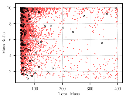
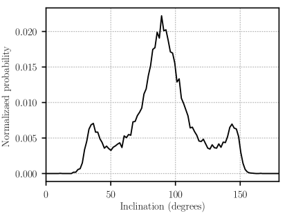
In Figure 2 we visualize the distribution of the waveforms in the template banks that we have created. The left panel of Figure 2 shows the distribution of the templates as a function of the total mass and mass ratio when including, and when not including, higher-order mode effects. As well as being able to see that many more templates are needed when including higher-order modes, we observe that we especially need many more templates at both high masses and high-mass ratios compared to the no higher-order modes bank where these regions are sparsely populated. In the right panel of Figure 2 we show the distribution of the inclination angle of higher-order mode waveforms in the template bank. We can see that many more templates are needed for edge-on systems than for face-on or face-away systems. We also observe two local maxima at $\sim 35$ and $\sim 135$ degrees. These peaks are an artifact of the two-stage template bank creation process, and the fact that templates are added to a set of non-higher-order mode waveforms, which will match well face-on and face-away systems.

V.2 Sensitivity comparison at fixed signal-to-noise ratio

Figure 3: The signal recovery fraction plotted as a function of the total mass and mass ratio. The top panels show results using a representative early Advanced LIGO sensitivity curve, while the bottom panels use the design Advanced LIGO sensitivity. The left panels are generated using appropriate template banks that do not include higher-order mode waveforms, the right panels are generated with template banks that include higher-order mode waveforms.

Figure 4: Left: Cumulative distribution of fitting factors for the 500,000 higher-order mode signal waveforms we describe in section V.2. The black curves show results for the Advanced LIGO design sensitivity curve and the red curves show results for the representative early Advanced LIGO sensitivity curve. Dotted lines indicate results when using template banks that do not include higher-order modes, solid lines show results using template banks including higher-order mode waveforms. Right: Distribution of fitting factors as a function of the source orientation $(\iota,\varphi)$ for $500$ signal waveforms with total mass of $95M_{\odot}$ and mass ratio of $8$.

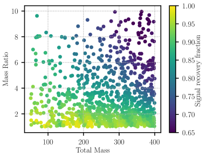
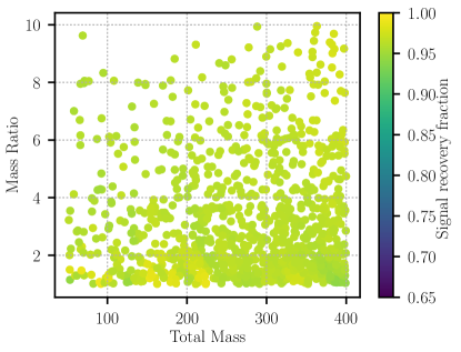
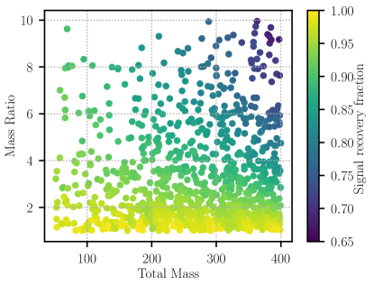
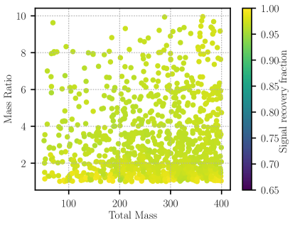
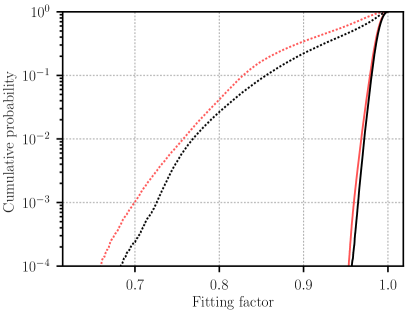
We wish to evaluate and compare the sensitivity to a set of given signals using both our template banks containing higher-order mode waveforms, and not containing them. This directly gives a measure of how much sensitivity would be gained by using our new higher-order mode search method. We first must define how this sensitivity will be computed. To assess the sensitivity to a given set of waveforms, drawn from some stated distribution, we must, for each waveform $g_{i}$ in the parameter space we consider, compute the fitting factor that will be recovered using the given template bank, composed of waveforms $b_{i}$. The distribution of fitting factors for the set of signals allows us to understand what fraction of signal-to-noise ratio we will recover for each waveform, and identify regions of parameter space where sensitivity is poor. However, it can often be misleading to only show the distribution of fitting factors, as often the systems for which fitting factors are smallest are also those ones whose observable gravitational-wave signal is weaker. To take into account the fact that different signals can be observed at different distances, one can define the corresponding “signal recovery fraction” of a given template bank $b_{i}$ to a distribution of signals $g_{i}$ as

$$\mathrm{SRF}=\frac{\sum_{i}\left(FF(g_{i},b_{j})\right)^{3}(g_{i}|g_{i})^{3}}{\sum_{i}(g_{i}|g_{i})^{3}}.$$ (17)

This was first introduced in terms of an “effective fitting factor” in Buonanno et al. (2003). One can understand the signal recovery fraction as the fraction of signals from a distribution $g_{i}$ that would be recovered above a fiducial signal-to-noise ratio threshold with the template bank $b_{i}$ compared to a template bank with a fitting factor of 1 for all $g_{i}$. For the plots shown in this section we compute the fitting factor, and then signal recovery fractions, using equation 14 to maximize over $u$. We have also created the plots using equation 13 and the numeric values agree to within $0.05\%$ with those in the plots shown. This demonstrates again that it is sufficient to use the computationally simpler equation 14 when performing a search using higher-order mode waveforms.

In Fig 3 we plot the signal recovery fraction as a function of the two component masses for both the early and design Advanced LIGO sensitivity curves, and for template banks with and without higher-order modes. For each point shown on this plot the signal recovery fraction is calculated by choosing a set of $g_{i}$ consisting of 500 waveforms. Each waveform has the same values of component masses, and the source orientations and sky locations are chosen isotropically. We show 1000 unique points in these plots, so a total of $500000$ waveforms are used in these simulations. We can clearly see in these plots that for equal mass systems the signal recovery fractions are large for template banks with and without higher-order modes. However, as the mass ratios become larger the signal recovery fraction can become as small as 0.65 when omitting higher-order modes, implying that ignoring higher-order modes in a search would result in a reduction in detection rate of up to 35% for systems with those masses. When we include higher-order mode waveforms, the signal recovery fractions are much more uniform, as expected. Values of 0.95 are consistent with the loss expected due to discreteness of the template bank. For the Advanced LIGO design sensitivity curve the effect of higher-order modes is smaller than that of the representative early Advanced LIGO noise curve. This is expected as the early Advanced LIGO noise curve is comparatively less sensitive at lower frequencies, where higher-order modes are less important. These results are consistent with earlier works exploring the effects of higher-order modes Pekowsky et al. (2013); Calderón Bustillo et al. (2016); Varma and Ajith (2016), reinforcing that higher-order modes are important for systems where the mass ratio and total mass is large.

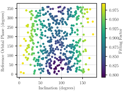
In Fig 4 we show the cumulative distribution of fitting factors for all of the $500000$ waveforms described above. This is shown for both the early and design Advanced LIGO sensitivity curves and for template banks both including and not including higher-order mode waveforms. We can clearly see here that there is a significant proportion of systems recovered with low fitting factors if higher-order modes are neglected. Using our higher-order mode template banks completely removes the tail of low fitting factors. We also show fitting factor as a function of the source orientation for all signals simulated at a total mass of $95M_{\odot}$ and a mass ratio of $8$. We can clearly see that the lowest fitting factors are obtained when the inclination angle is edge-on, as expected.

V.3 Sensitivity comparison at fixed false-alarm rate

Bank	SNR threshold at false-alarm rate of $10^{-3}yr^{-1}$	SNR threshold at false-alarm rate of $0.5\times 10^{-3}yr^{-1}$
Early, no HOM	9.10	9.16
Early, with HOM	Not applicable	9.68
Design, no HOM	9.31	9.37
Design, with HOM	Not applicable	9.70

Table 2: Signal-to-noise ratio thresholds at the false-alarm rate values used in this study for the various template banks and sensitivity curves considered. “Early” refers to the representative sensitivity curve from Advanced LIGO’s first observing run, “Design” refers to Advanced LIGO’s design sensitivity. “HOM” stands for “higher-order modes”, “SNR” stands for “signal-to-noise ratio”.

Figure 5: The sensitivity ratio between a search using higher-order mode waveforms as templates and a search using non-higher-order-mode waveforms as templates, evaluating sensitivity using only signal-to-noise ratio to rank potential events. Plotted for the early Advanced LIGO sensitivity curve (left) and the Advanced LIGO design sensitivity curve (right). The plots on the top row consider the full injection set, while plots on the bottom row consider only injections where the inclination ($\iota$) is between 60 and 120 degrees. The sensitivity is evaluated at a false-alarm rate of 1 per 1000 years, which includes the larger background that is present when using higher-order mode waveforms as templates, as more template waveforms are needed. Values greater than one indicate an increase in sensitivity, values less than one indicate a decrease in sensitivity.

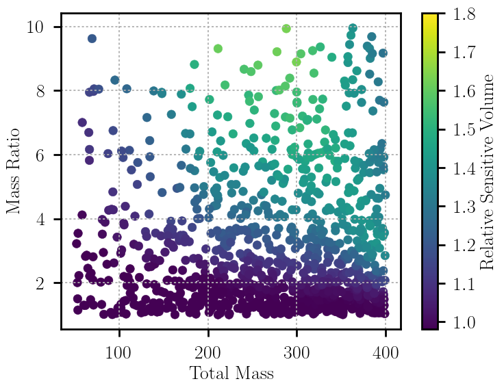
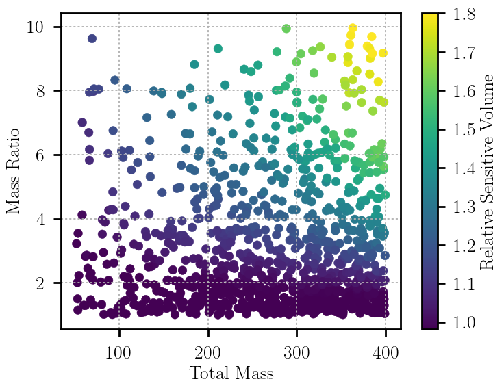
The results in section V.2 demonstrate that when including higher-order mode effects in the waveform filters used in a search the search efficiency will increase when evaluating efficiency above a constant signal-to-noise ratio threshold. However, in a real search the signal-to-noise ratio threshold is a function of the number of waveform templates, and the size of the parameter space covered. Our higher-order mode template banks are roughly an order of magnitude larger than the corresponding non-higher-order mode template banks. This increase in the number of templates will increase the rate of background events in the search, and therefore a signal would require a larger signal-to-noise ratio to achieve the same significance, when evaluated in terms of a false-alarm rate. In this section we will assess the sensitivity increase that can be obtained when using our higher-order mode template banks, at a constant false-alarm-rate threshold, which takes into account the increase in background triggers from using a larger number of template waveforms.

The first step is to create a mapping between signal-to-noise ratio and false-alarm rate. We do this for each of our template banks by simulating $\sim 5$ days of Gaussian noise with either the representative early Advanced LIGO sensitivity curve or the Advanced LIGO design sensitivity curve. We then analyse this data with the various template banks using the PyCBC analysis framework Dal Canton et al. (2014); Usman et al. (2015); Nitz et al. (2017b), which allows us to directly map the signal-to-noise ratio to a false-alarm rate. A false-alarm weighted relative signal-recovery fraction can then be computed according to

$$\mathrm{SRF}=\frac{\sum_{i}\left(FF(g_{i},b_{j})\right)^{3}(g_{i}|g_{i})^{3}}{\rho_{\mathrm{thresh}}^{3}\sum_{i}(g_{i}|g_{i})^{3}},$$ (18)

where $\rho_{\mathrm{thresh}}$ is the signal-to-noise threshold corresponding to the desired false-alarm rate. This doesn’t have meaning as a statistic on it’s own, but the ratio of this quantity computed for two different searches, which will have different values of fitting factor and $\rho_{\mathrm{thresh}}$, directly gives the relative sensitivity. One could compute this directly for our higher-order mode, and non-higher-order mode template banks. However, this would result in a non-negligible decrease in sensitivity in the equal mass region of parameter space. This is because this region of parameter space is already well recovered by non-higher-order mode waveforms and the increased signal-to-noise ratio threshold, due to the higher-order mode waveforms, only causes a reduction in sensitivity for equal-mass systems. Instead, we can choose to consider two separate searches, one with higher-order modes and one without, and combine the results together, including the necessary trials factor of 2. This would limit the decrease in sensitivity to $\sim 1\%$ in regions where higher-order modes contribute nothing while still allowing a sensitivity increase where higher-order modes are important. Formally the false-alarm weighted relative signal-recovery fraction for this combined search would be computed according to

$$\mathrm{SRF}_{\mathrm{combined}}=\left(\frac{\sum_{i}(\mathrm{FF_{weighted}})_{i}(g_{i}|g_{i})^{3}}{\sum_{i}(g_{i}|g_{i})^{3}}\right),$$ (19)

where we define

$$(\mathrm{FF_{weighted}})_{i}=\max_{j}\left\{(\rho_{\mathrm{thresh}})_{j}^{-3}\textrm{FF}_{i,j}^{3}\right\},$$ (20)

where $j$ denotes the values for the two searches being performed.

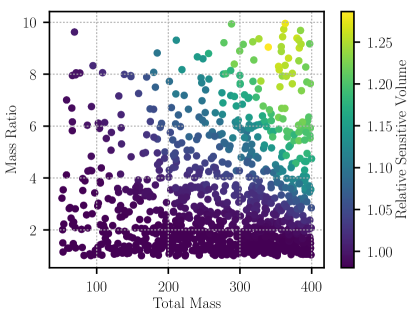
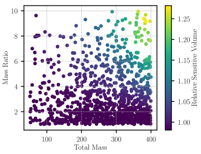
In Table 2 we show the network signal-to-noise ratios corresponding to a false-alarm rate of $10^{-3}yr^{-1}$. This is the threshold at which we choose to evaluate the relative sensitivity of our higher-order mode search. When computing the combined search sensitivity we incorporate the trials factor by using a false-alarm rate of $0.5\times 10^{-3}yr^{-1}$ in each search, and therefore $10^{-3}yr^{-1}$ in the combined search. To the accuracies quoted in this table, the threshold obtained is the same if we use equation 14 or equation 13 to maximize over $u$. In Figure 5 we show the sensitivity increase between the higher-order mode and non-higher-order mode searches as a function of the total mass and mass ratio. This is computed from the same set of waveforms as used in Figure 3. We see that in both cases there is no increase in sensitivity for equal mass systems but an increase in sensitivity of up to 25% for the systems with the highest total mass and mass ratio that we consider here. It is important to again emphasize that while these averaged sensitivity increases are modest, even a single observation of a compact binary merger with measurable higher-order mode emission would allow for much more precise measurement of source parameters than systems where only the dominant gravitational-wave emission modes are observable Varma et al. (2014); Graff et al. (2015); Calderón Bustillo et al. (2016); Varma and Ajith (2016). In this sense, we stress that we are presenting a gain in sensitivity which is averaged over the possible orientations of the binary. These results are often dominated by face-on binaries, which have a stronger emission, and for which the quadrupolar bank shows an excellent signal recovery. The sensitivity gain is much larger for edge-on binaries, whose emission has a strong higher mode contribution, leading to a poor signal recovery when a quadrupolar bank is used as demonstrated in Figure 4. To emphasize this, in the lower panel of Figure 3 we also show the sensitivity increase if considering only those waveforms with $60^{\circ}<\iota<120^{\circ}$, which are those waveforms oriented edge-on to the observer and for which higher-modes are most important. Here we observe much higher sensitivity increases—up to 80%—than with the full set of simulated waveforms.

We note that equation 19 defines a simple measure for combining the higher-order mode and non-higher-order mode searches, which does not reduce significantly the sensitivity to non-higher-order mode waveforms, while simultaneously allowing a sensitivity increase for systems where higher-order modes are important. However, a more optimal method to combine these two searches, would be to utilize a method similar to that defined in Dent and Veitch (2014), which uses Bayesian methodology to weight each template waveform according to its probability of observing a system. However, such a method requires a good knowledge of the astrophysical distribution of systems, which is not known for intermediate-mass black hole binary systems, and requires knowing relatively how often each template is to observe a signal, which is difficult to compute with curved and degenerate parameter spaces where it can be difficult to determine what region of parameter space is best covered by each template.

VI Real data concerns for searches for high-mass waveforms

In the previous sections we have evaluated the sensitivity increase when using filter waveforms containing higher-order modes assuming that the detector noise is Gaussian and stationary and using only the signal-to-noise ratio to evaluate the significance of events. In reality, data taken from gravitational-wave observatories is neither Gaussian nor stationary and instrumental non-Gaussian noise transients will produce large values of signal-to-noise ratio in a matched-filter search Aasi et al. (2012, 2015b); Abbott et al. (2016g). Therefore search strategies for compact binary coalescences must take into account such non-Gaussian transients and be able to distinguish them from genuine astrophysical signals. There are numerous works that have focused on this problem Allen et al. (2012); Harry and Fairhurst (2011); Babak et al. (2013); Biswas et al. (2013); Messick et al. (2017); Nitz et al. (2017a). However, many of these tests were created considering lower mass compact binary mergers than those considered here and these tests are known to be less efficient when searching for intermediate-mass black hole binary mergers Abbott et al. (2017b). Some tests are beginning to focus on the efficiency to higher mass black hole binary mergers, but are not yet able to separate all forms of transient noise, and are not fully tuned for higher-order mode waveforms Nitz (2017).

Indeed for certain regions of the parameter space unmodelled search techniques have been found to be more sensitive to compact binary mergers in data from LIGO’s first observing run than modelled searches, because they are better at removing instrumental artifacts Mohapatra et al. (2014); Calderon Bustillo et al. (2017). Optimizing searches to better distinguish real astrophysical signals from instrumental noise at high masses is an interesting topic that should be addressed, but this should be done in a separate work, and we will not attempt to address this specific question here.

In this section we will explore how existing tests to separate real signals from noise artifacts can be applied when using higher-order mode waveforms, we will demonstrate that these tests can misclassify genuine astrophysical signals with significant higher-order mode contribution as instrumental artifacts, and that this problem is significantly mitigated when using higher-order mode waveforms as filters in the search.

VI.1 Reweighted signal-to-noise ratio

Figure 6: Impact of higher-modes on the $\chi^{2}$ signal consistency test. We plot $\chi^{2}$ against signal-to-noise ratio for a randomly chosen subset of the simulated signals discussed in section VI. The inclination angle of the simulated signals are shown on the colorbar, here we restrict the inclination angle to values between 0 and $\pi/2$ by taking $\pi/2-|\pi/2-\iota|$. The dashed lines denote contours of equal $\rho_{\mathrm{reweighted}}$. The left panel shows the results when searching with a template bank that does not include higher-order mode waveforms, the right panel shows the results when searching with higher-order mode templates. Both panels are generated using the design Advanced LIGO sensitivity curves.

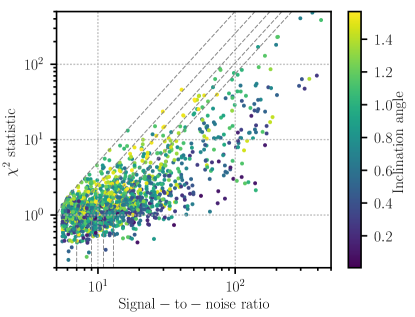
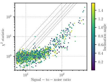
One of the most common methods for discriminating between gravitational wave triggers and noise artifacts is to check whether the morphology of a potential signal in the data, $s$, is consistent with that of the filter waveform being used, $h$. Several methods for doing this, testing different features of the potential signal’s morphology, have been proposed Allen et al. (2012); Harry and Fairhurst (2011); Babak et al. (2013); Messick et al. (2017). Of these, arguably the most effective test is the one described in Allen et al. (2012). In that test a number of filters are constructed from the template waveform $h$ in the following way. A set of $N$ filters $h_{i}$ is chosen such that each $h_{i}$ is constructed, in the frequency domain as

$$\tilde{h}_{i}(f)=\begin{cases}\tilde{h}(f)&\mathrm{for}\ f_{L}<f<=f_{U}\\ 0&\mathrm{otherwise}\end{cases}.$$ (21)

Each filter $h_{i}$ uses non-overlapping frequency windows, $f_{L}$ and $f_{U}$, such that $\sum_{i}h_{i}=h$. Also $(h_{i}|h_{i})=(h_{j}|h_{j})$ for any value of $i$ and $j$ and $(h_{i}|h_{j})=0$ for any $i\neq j$. By this definition if the data $s$ is a good match to the filter waveform then each of the $h_{i}$ should recover the same signal-to-noise ratio, within deviations expected in Gaussian noise. In contrast, noise artifacts are often well localized in time and would often produce a very large signal-to-noise ratio in a small number of $h_{i}$ and a small signal-to-noise ratio in the rest. Therefore one can construct a chi-squared test as

$$\chi^{2}=\frac{N}{\langle h|h\rangle}\sum_{i=1}^{N}\left\|\langle s|h_{i}\rangle-\frac{\langle s|h\rangle}{N}\right\|^{2}.$$ (22)

If $s$ is described by Gaussian noise with an added signal well modelled by $h$, this will follow a $\chi^{2}$ distribution with $2N-2$ degrees of freedom Allen et al. (2012). For non-Gaussian artifacts it has been empirically demonstrated that this will take larger values Allen et al. (2012); Babak et al. (2013), allowing for separation between real signals and Gaussian artifacts. There are a number of different techniques for combining the $\chi^{2}$ test with the signal-to-noise ratio to produce a ranking statistic Babak et al. (2013); Adams et al. (2016); Messick et al. (2017); Nitz et al. (2017a), we choose to use here the combination described in Babak et al. (2013), which has been used to analyse Advanced LIGO data with the PyCBC analysis method Abadie et al. (2012). This “reweighted signal-to-noise ratio” is given by Babak et al. (2013)

$$\rho_{\mathrm{reweighted}}=\begin{cases}\rho&\mathrm{for}\ \chi^{2}<=n_{\mathrm{d}}\\ \rho\left[\frac{1}{2}\left(1+\left(\frac{\chi^{2}}{n_{\mathrm{d}}}\right)^{3}\right)\right]^{1/6}&\mathrm{for}\ \chi^{2}>n_{\mathrm{d}}\end{cases},$$ (23)

where $n_{\mathrm{d}}=2N-2$. We want to explore how well this reweighted signal-to-noise ratio performs when searching for higher-order mode signals with and without higher-order mode filter waveforms.

VI.2 Sensitivity comparison at fixed false-alarm rate with reweighted signal-to-noise ratio

Figure 7: The relative sensitivity between a search using higher-order mode waveforms as templates and a search using non-higher-order-mode waveforms as templates when evaluating sensitivity using $\rho_{\mathrm{reweighted}}$ at a constant rate of false alarm. Plotted for the representative early Advanced LIGO sensitivity curve (left) and the design Advanced LIGO sensitivity curve (right). The plots on the top row consider the full injection set, while plots on the bottom row consider only injections where the inclination ($\iota$) is between 60 and 120 degrees. The sensitivity is evaluated at a false-alarm rate of 1 per 1000 years, which includes the larger background that is present when using higher-order mode waveforms as templates. Values greater than one indicate an increase in sensitivity, values less than one indicate a decrease in sensitivity. Here the color bars are capped at a value of 2 to aid distinguishability of values between 1 and 2. However some values are larger than this, especially in the lower right panel, where the points with highest mass and highest mass ratio have a relative sensitive volume of $\sim$ 4.

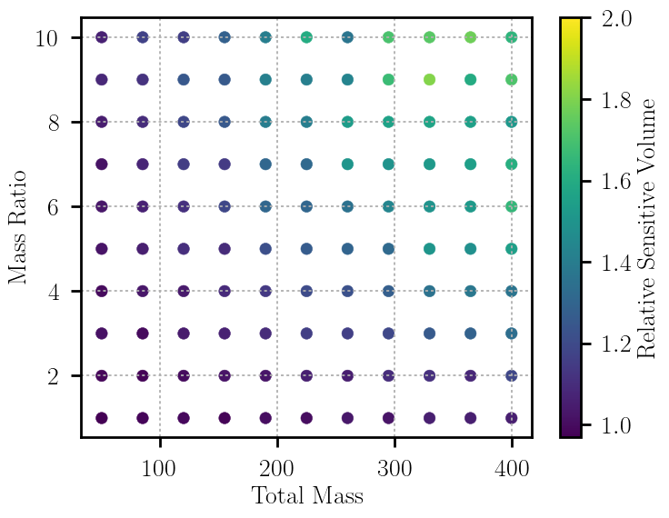
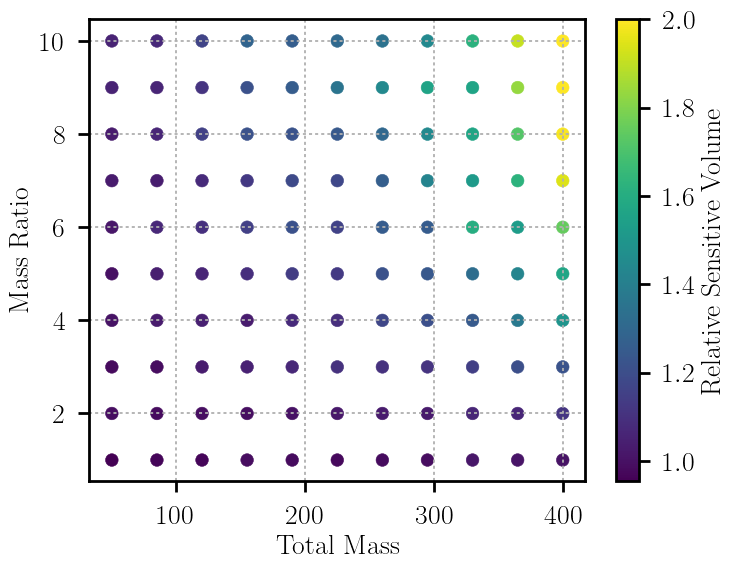
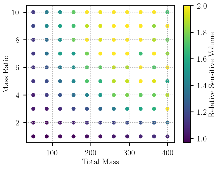
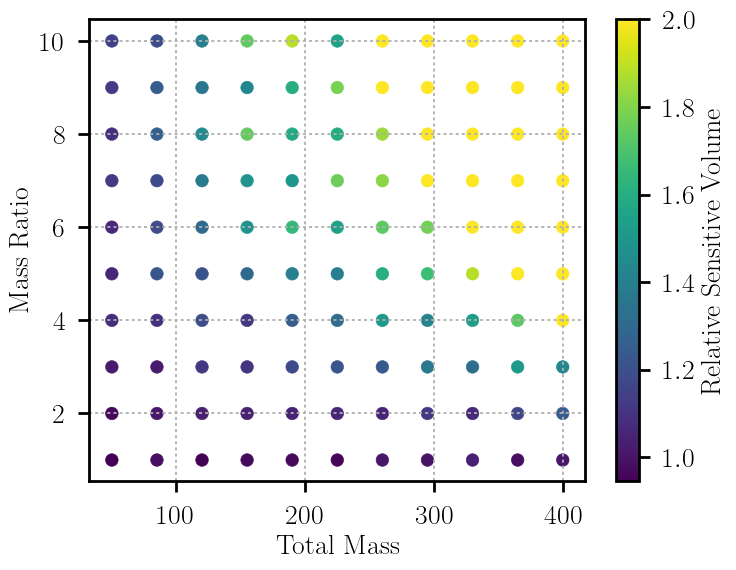
We generate a large set of simulated intermediate-mass black hole binary waveforms to assess the sensitivity of our higher-order mode search method when evaluating sensitivity using the reweighted signal-to-noise ratio defined above. We use the same distribution of parameters as described in the section V, but as the values of the $\chi^{2}$ test will depend on the amplitude of the signal, we include the distance and sky location as parameters when generating the simulation set. We also add the simulated signals to simulated Gaussian noise when measuring the signal-to-noise ratio and $\chi^{2}$. The signals are added to noise simulating both Advanced LIGO observatories and the quadrature sum of the recovered $\rho_{\mathrm{reweighted}}$ is used to rank events. In total we choose to simulate signals with $110$ unique masses and using $\sim 10000$ unique simulated signals for each mass.

In Figure 6 we show the distribution of $\chi^{2}$ values as a function of signal-to-noise ratio, both with and without higher-order mode filter waveforms. The dashed lines show contours of constant $\rho_{\mathrm{reweighted}}$; the $\rho_{\mathrm{reweighted}}$ increases as the signal-to-noise ratio increases and as the value of the $\chi^{2}$ test decreases. When searching for systems that are oriented face-on to the observer using non-higher-order mode filter waveforms the $\chi^{2}$ values tend to be low as the higher-order mode content is negligible. However, as the inclination $\iota$ increases, higher-modes contribute more to the resulting signal, increasing the mismatch between signal and template and causing the $\chi^{2}$ to grow. When using higher-order mode filter waveforms the $\chi^{2}$ values are lower, and lie away from the contour lines where non-Gaussian artifacts would appear in real data. The $\chi^{2}$ test would therefore cause an additional loss in sensitivity over that considered in section V if searching for higher-order mode waveforms using filters that neglect higher-order modes.

We therefore reproduce the figures shown in Figure 5, but using $\rho_{\mathrm{reweighted}}$ to rank potential events instead of using signal-to-noise ratio. This is shown in Figure 7. We see in this plot a larger sensitivity increase when including higher-order modes compared to that seen in Figure 5 due to the effect of the $\chi^{2}$ test. We also now see a larger sensitivity increase for the design Advanced LIGO sensitivity curve, whereas previously the larger sensitivity increase was seen with the early Advanced LIGO sensitivity curve. This indicates that the $\chi^{2}$ test is misclassifying more systems for the design sensitivity curve than for the early curve. These results qualitatively match the results in Capano et al. (2014) where the authors made predictions of how the sensitivity should increase if one were able to include higher-order mode waveforms as filters in a search. As with Figure 5, we also show results considering only injections aligned close to edge-on to the observer in the lower panels. As before, we observe much larger sensitivity increases, and again this increase is larger when including the effects of the $\chi^{2}$ test. In Figure 7 we chose to set the maximum value on the colorbar to 2 to allow the reader to observe improvements in sensitivity that are less than 1.5. However there are some values that are much larger than this, up to a value of 4—indicating a 300% increase in the number of observed signals—for the points with the largest mass and largest mass ratio in the lower right panel. In such regions our new higher-order mode search is especially needed.

While it would be beneficial to work on exploring and tuning various signal-based consistency tests and classifiers to improve the performance of searching for higher-order-mode waveforms with template waveforms that do not include higher-order modes, such tests and classifiers will be more powerful if the template waveforms being used match well to the signals in the data. Some more work is needed to improve the separation of noise transients from real signals, in the intermediate-mass black hole binary parameter space, and in the case where the template waveforms match well. However, we recommend that such work is performed while using waveforms that include higher-order mode waveforms, as described in this work.

VII Conclusions

In this work we have presented a new method for searching for compact binary coalescences using filter waveforms which include higher-order mode gravitational-wave emission. This method will allow for the first time searches using higher-order mode filter waveforms to be performed in ongoing analysis of data from second-generation gravitational-wave observatories. We have demonstrated the sensitivity improvement this method would allow. This improvement is as much as a 100% improvement for systems with mass ratios of 10 and total mass of 400 $M_{\odot}$, but is much more modest, $<10\%$, for systems with equal mass or with total mass of 50 $M_{\odot}$. In the cases where the improvement is modest, it implies that the efficiency of the current, non-higher order mode search, is already good in these areas. The improvement in sensitivity is largest—as much as 300%—for systems oriented edge-on to the observer, which are intrinsically fainter in gravitational-waves than face-on systems, but for which higher-order modes are especially important. The detection of such signals is key for testing fundamental aspects of General Relativity. For instance, a clear observation of at least two ringdown modes is needed for testing the no-hair theorem Dreyer et al. (2004); Maselli et al. (2017). The method we present is also fully generic and could be applied also in searches for eccentric, or precessing, compact binary mergers.

Using this method to search for higher-order mode signals in the latest Advanced LIGO and Advanced Virgo data would require waveform models that include both higher-order mode emission and model the effect of the components’ spins. At the time of writing such waveform models are not available, but are currently in rapid development London et al. (2017); Cotesta et al. (2017). When these waveform models are available it is trivial to extend the results shown here to include the component spins, although the size of both higher-order mode and non-higher-order mode template banks will increase when including this additional freedom. Nevertheless, we see no reason why one wouldn’t expect the same relative sensitivity improvement as seen here with non-spinning waveform models, when using spinning higher-order mode waveforms.

A current problem with searches for intermediate-mass black hole binary mergers is that the gravitational emission from such systems is only observed for a very short time and can be confused with non-Gaussian noise transients. Developing better techniques to distinguish between noise transients and genuine gravitational-wave signals would be very beneficial in this search space, although this task is orthogonal to the problem addressed in this paper. We have also demonstrated that the performance of current signal-based consistency tests is improved significantly by including higher-order mode effects in the search parameter space.

VIII Acknowledgements

The authors would like to thank Stas Babak, Alejandro Bohé, Alessandra Buonanno, Collin Capano, Sylvain Marsat, Stephen Privitera and Vivien Raymond for helpful discussions. The authors also thank Collin Capano for reading through the manuscript and providing useful feedback and comments. The authors would also like to thank the anonymous referees for carefully reading this manuscript and providing useful comments, suggestions and feedback. IH and AN would like to thank the Max Planck Gesellschaft for support. JCB gratefully acknowledges support from the NSF grants 1505824, 1505524 and 1333360. Computations used in this work were performed on the “Vulcan” and “Atlas” high-throughput computing clusters operated by the Max Planck Institute for Gravitational Physics.

References

- Aasi et al. (2015a) J. Aasi et al. (LIGO Scientific), Class. Quant. Grav. 32, 074001 (2015a), arXiv:1411.4547 [gr-qc] .
- Abbott et al. (2016a) B. P. Abbott et al. (Virgo, LIGO Scientific), Phys. Rev. Lett. 116, 061102 (2016a), arXiv:1602.03837 [gr-qc] .
- Abbott et al. (2016b) B. Abbott et al. (Virgo, LIGO Scientific), Phys. Rev. Lett. 116, 241103 (2016b), arXiv:1606.04855 [gr-qc] .
- Abbott et al. (2017a) B. Abbott et al. (VIRGO, LIGO Scientific), Phys. Rev. Lett. 118, 221101 (2017a).
- Acernese et al. (2015) F. Acernese et al. (VIRGO), Class. Quant. Grav. 32, 024001 (2015), arXiv:1408.3978 [gr-qc] .
- Aso et al. (2013) Y. Aso, Y. Michimura, K. Somiya, M. Ando, O. Miyakawa, T. Sekiguchi, D. Tatsumi, and H. Yamamoto (KAGRA), Phys. Rev. D88, 043007 (2013), arXiv:1306.6747 [gr-qc] .
- Iyer et al. (2011) B. Iyer et al., “LIGO-India, Proposal of the Consortium for Indian Initiative in Gravitational-wave Observations (IndIGO),” (2011), https://dcc.ligo.org/LIGO-M1100296/public.
- Abbott et al. (2016c) B. P. Abbott et al. (VIRGO, LIGO Scientific), Living Rev. Rel. 19, 1 (2016c), arXiv:1304.0670 [gr-qc] .
- Abbott et al. (2016d) B. P. Abbott et al. (Virgo, LIGO Scientific), Astrophys. J. 833, L1 (2016d), arXiv:1602.03842 [astro-ph.HE] .
- Abbott et al. (2016e) B. P. Abbott et al. (Virgo, LIGO Scientific), Phys. Rev. Lett. 116, 241102 (2016e), arXiv:1602.03840 [gr-qc] .
- Abbott et al. (2016f) B. P. Abbott et al. (Virgo, LIGO Scientific), (2016f), arXiv:1606.04856 [gr-qc] .
- Amaro-Seoane and Santamaria (2010) P. Amaro-Seoane and L. Santamaria, Astrophys. J. 722, 1197 (2010), arXiv:0910.0254 [astro-ph.CO] .
- Amaro-Seoane (2012) P. Amaro-Seoane, (2012), arXiv:1205.5240 [astro-ph.CO] .
- Gair et al. (2011) J. R. Gair, I. Mandel, M. C. Miller, and M. Volonteri, Gen. Rel. Grav. 43, 485 (2011), arXiv:0907.5450 [astro-ph.CO] .
- Sesana et al. (2009) A. Sesana, J. Gair, I. Mandel, and A. Vecchio, Astrophys. J. 698, L129 (2009), arXiv:0903.4177 [astro-ph.CO] .
- Volonteri (2012a) M. Volonteri, Proceedings, 4th Meeting on First stars IV: From Hayashi to the future: Kyoto, Japan, May 21-25, 2012, AIP Conf. Proc. 1480, 289 (2012a), arXiv:1209.1195 [astro-ph.CO] .
- Volonteri (2012b) M. Volonteri, Science 337, 544 (2012b), arXiv:1208.1106 [astro-ph.CO] .
- Nitz et al. (2017a) A. H. Nitz, T. Dent, T. Dal Canton, S. Fairhurst, and D. A. Brown, (2017a), arXiv:1705.01513 [gr-qc] .
- Usman et al. (2015) S. A. Usman et al., (2015), arXiv:1508.02357 [gr-qc] .
- Dal Canton et al. (2014) T. Dal Canton, A. H. Nitz, A. P. Lundgren, A. B. Nielsen, D. A. Brown, et al., Phys.Rev. D90, 082004 (2014), arXiv:1405.6731 [gr-qc] .
- Cannon et al. (2012) K. Cannon, R. Cariou, A. Chapman, M. Crispin-Ortuzar, N. Fotopoulos, et al., Astrophys.J. 748, 136 (2012), arXiv:1107.2665 [astro-ph.IM] .
- Cannon et al. (2013) K. Cannon, C. Hanna, and D. Keppel, Phys.Rev. D88, 024025 (2013), arXiv:1209.0718 [gr-qc] .
- Sathyaprakash and Dhurandhar (1991) B. S. Sathyaprakash and S. V. Dhurandhar, Phys. Rev. D44, 3819 (1991).
- Babak et al. (2006) S. Babak, R. Balasubramanian, D. Churches, T. Cokelaer, and B. S. Sathyaprakash, Class. Quant. Grav. 23, 5477 (2006), arXiv:gr-qc/0604037 [gr-qc] .
- Ajith et al. (2014) P. Ajith, N. Fotopoulos, S. Privitera, A. Neunzert, and A. J. Weinstein, Phys. Rev. D89, 084041 (2014), arXiv:1210.6666 [gr-qc] .
- Brown et al. (2012) D. A. Brown, I. Harry, A. Lundgren, and A. H. Nitz, Phys. Rev. D86, 084017 (2012), arXiv:1207.6406 [gr-qc] .
- Capano et al. (2016) C. Capano, I. Harry, S. Privitera, and A. Buonanno, Phys. Rev. D93, 124007 (2016), arXiv:1602.03509 [gr-qc] .
- Pretorius (2005) F. Pretorius, Phys.Rev.Lett. 95, 121101 (2005), arXiv:gr-qc/0507014 [gr-qc] .
- Szilagyi et al. (2009) B. Szilagyi, L. Lindblom, and M. A. Scheel, Phys.Rev. D80, 124010 (2009), arXiv:0909.3557 [gr-qc] .
- Scheel et al. (2009) M. A. Scheel, M. Boyle, T. Chu, L. E. Kidder, K. D. Matthews, et al., Phys.Rev. D79, 024003 (2009), arXiv:0810.1767 [gr-qc] .
- Frauendiener (2011) J. Frauendiener, Gen.Rel.Grav. 43, 2931 (2011).
- Hannam et al. (2010) M. Hannam, S. Husa, F. Ohme, D. Muller, and B. Bruegmann, Phys.Rev. D82, 124008 (2010), arXiv:1007.4789 [gr-qc] .
- Chu (2011) T. Chu, Numerical simulations of black-hole spacetimes, Ph.D. thesis, Caltech (2011).
- Vaishnav et al. (2007) B. Vaishnav, I. Hinder, F. Herrmann, and D. Shoemaker, Phys. Rev. D76, 084020 (2007), arXiv:0705.3829 [gr-qc] .
- Herrmann et al. (2007) F. Herrmann, I. Hinder, D. Shoemaker, and P. Laguna, New frontiers in numerical relativity. Proceedings, International Meeting, NFNR 2006, Potsdam, Germany, July 17-21, 2006, Class. Quant. Grav. 24, S33 (2007), arXiv:gr-qc/0601026 [gr-qc] .
- Healy et al. (2009) J. Healy, J. Levin, and D. Shoemaker, Phys. Rev. Lett. 103, 131101 (2009), arXiv:0907.0671 [gr-qc] .
- Blanchet et al. (1995) L. Blanchet, T. Damour, B. R. Iyer, C. M. Will, and A. Wiseman, Phys.Rev.Lett. 74, 3515 (1995), arXiv:gr-qc/9501027 [gr-qc] .
- Buonanno and Damour (1999) A. Buonanno and T. Damour, Phys.Rev. D59, 084006 (1999), arXiv:gr-qc/9811091 [gr-qc] .
- Taracchini et al. (2012) A. Taracchini, Y. Pan, A. Buonanno, E. Barausse, M. Boyle, et al., Phys.Rev. D86, 024011 (2012), arXiv:1202.0790 [gr-qc] .
- Bohé et al. (2017) A. Bohé et al., Phys. Rev. D95, 044028 (2017), arXiv:1611.03703 [gr-qc] .
- Ajith et al. (2008) P. Ajith, S. Babak, Y. Chen, M. Hewitson, B. Krishnan, et al., Phys.Rev. D77, 104017 (2008), arXiv:0710.2335 [gr-qc] .
- Khan et al. (2016) S. Khan, S. Husa, M. Hannam, F. Ohme, M. Pürrer, X. Jiménez Forteza, and A. Bohé, Phys. Rev. D93, 044007 (2016), arXiv:1508.07253 [gr-qc] .
- Apostolatos et al. (1994) T. A. Apostolatos, C. Cutler, G. J. Sussman, and K. S. Thorne, Phys. Rev. D49, 6274 (1994).
- Damour et al. (2004) T. Damour, A. Gopakumar, and B. R. Iyer, Phys. Rev. D70, 064028 (2004), arXiv:gr-qc/0404128 [gr-qc] .
- Flanagan and Hinderer (2008) E. E. Flanagan and T. Hinderer, Phys. Rev. D77, 021502 (2008), arXiv:0709.1915 [astro-ph] .
- Read et al. (2013) J. S. Read, L. Baiotti, J. D. E. Creighton, J. L. Friedman, B. Giacomazzo, K. Kyutoku, C. Markakis, L. Rezzolla, M. Shibata, and K. Taniguchi, Phys. Rev. D88, 044042 (2013), arXiv:1306.4065 [gr-qc] .
- Blanchet et al. (2008) L. Blanchet, G. Faye, B. R. Iyer, and S. Sinha, Class.Quant.Grav. 25, 165003 (2008), arXiv:0802.1249 [gr-qc] .
- O’Shaughnessy et al. (2014) R. O’Shaughnessy, B. Farr, E. Ochsner, H.-S. Cho, V. Raymond, C. Kim, and C.-H. Lee, Phys. Rev. D89, 102005 (2014), arXiv:1403.0544 [gr-qc] .
- McKechan (2011) D. J. A. McKechan, On the use of higher order waveforms in the search for gravitational waves emitted by compact binary coalescences, Ph.D. thesis, Cardiff U. (2011), arXiv:1102.1749 [gr-qc] .
- Pekowsky et al. (2013) L. Pekowsky, J. Healy, D. Shoemaker, and P. Laguna, Phys.Rev. D87, 084008 (2013), arXiv:1210.1891 [gr-qc] .
- Capano et al. (2014) C. Capano, Y. Pan, and A. Buonanno, Phys.Rev. D89, 102003 (2014), arXiv:1311.1286 [gr-qc] .
- Varma et al. (2014) V. Varma, P. Ajith, S. Husa, J. C. Bustillo, M. Hannam, et al., (2014), arXiv:1409.2349 [gr-qc] .
- Calderón Bustillo et al. (2016) J. Calderón Bustillo, S. Husa, A. M. Sintes, and M. Pürrer, Phys. Rev. D93, 084019 (2016), arXiv:1511.02060 [gr-qc] .
- Calderón Bustillo et al. (2017) J. Calderón Bustillo, P. Laguna, and D. Shoemaker, Phys. Rev. D95, 104038 (2017), arXiv:1612.02340 [gr-qc] .
- Klimenko et al. (2008) S. Klimenko, I. Yakushin, A. Mercer, and G. Mitselmakher, Proceedings, 18th International Conference on General Relativity and Gravitation (GRG18) and 7th Edoardo Amaldi Conference on Gravitational Waves (Amaldi7), Sydney, Australia, July 2007, Class. Quant. Grav. 25, 114029 (2008), arXiv:0802.3232 [gr-qc] .
- Sutton et al. (2010) P. J. Sutton et al., New J. Phys. 12, 053034 (2010), arXiv:0908.3665 [gr-qc] .
- Cornish and Littenberg (2015) N. J. Cornish and T. B. Littenberg, Class. Quant. Grav. 32, 135012 (2015), arXiv:1410.3835 [gr-qc] .
- Lynch et al. (2017) R. Lynch, S. Vitale, R. Essick, E. Katsavounidis, and F. Robinet, Phys. Rev. D95, 104046 (2017), arXiv:1511.05955 [gr-qc] .
- Klimenko et al. (2016) S. Klimenko et al., Phys. Rev. D93, 042004 (2016), arXiv:1511.05999 [gr-qc] .
- Mazzolo et al. (2014) G. Mazzolo et al., Phys. Rev. D90, 063002 (2014), arXiv:1404.7757 [gr-qc] .
- Pan et al. (2011) Y. Pan, A. Buonanno, M. Boyle, L. T. Buchman, L. E. Kidder, H. P. Pfeiffer, and M. A. Scheel, Phys. Rev. D84, 124052 (2011), arXiv:1106.1021 [gr-qc] .
- London et al. (2017) L. London, S. Khan, E. Fauchon-Jones, X. J. Forteza, M. Hannam, S. Husa, C. Kalaghatgi, F. Ohme, and F. Pannarale, (2017), arXiv:1708.00404 [gr-qc] .
- Cotesta et al. (2017) R. Cotesta et al., In preparation (2017).
- Gossan et al. (2012) S. Gossan, J. Veitch, and B. S. Sathyaprakash, Phys. Rev. D85, 124056 (2012), arXiv:1111.5819 [gr-qc] .
- Yang et al. (2017) H. Yang, K. Yagi, J. Blackman, L. Lehner, V. Paschalidis, F. Pretorius, and N. Yunes, Phys. Rev. Lett. 118, 161101 (2017), arXiv:1701.05808 [gr-qc] .
- Berti et al. (2015) E. Berti et al., Class. Quant. Grav. 32, 243001 (2015), arXiv:1501.07274 [gr-qc] .
- Sigg (2016) D. Sigg, “Advanced LIGO first observing run representative sensitivity,” (2016), https://dcc.ligo.org/LIGO-G1600150/public https://dcc.ligo.org/LIGO-G1600151/public.
- Shoemaker (2015) D. Shoemaker, “Advanced ligo anticipated sensitivity curves,” (2015), https://dcc.ligo.org/LIGO-T0900288/public.
- Finn and Chernoff (1993) L. S. Finn and D. F. Chernoff, Phys. Rev. D47, 2198 (1993), arXiv:gr-qc/9301003 [gr-qc] .
- Jaranowski et al. (1998) P. Jaranowski, A. Krolak, and B. F. Schutz, Phys.Rev. D58, 063001 (1998), arXiv:gr-qc/9804014 [gr-qc] .
- Goldberg et al. (1967) Goldberg et al., J. Math. Phys. 8:2155–2161 (1967).
- Healy et al. (2013) J. Healy, P. Laguna, L. Pekowsky, and D. Shoemaker, Phys. Rev. D88, 024034 (2013), arXiv:1302.6953 [gr-qc] .
- Bustillo et al. (2015) J. C. Bustillo, A. Bohé, S. Husa, A. M. Sintes, M. Hannam, et al., (2015), arXiv:1501.00918 [gr-qc] .
- Damour et al. (2013) T. Damour, A. Nagar, and S. Bernuzzi, Phys.Rev. D87, 084035 (2013), arXiv:1212.4357 [gr-qc] .
- Santamaria et al. (2010) L. Santamaria, F. Ohme, P. Ajith, B. Bruegmann, N. Dorband, et al., Phys.Rev. D82, 064016 (2010), arXiv:1005.3306 [gr-qc] .
- Hannam et al. (2014) M. Hannam, P. Schmidt, A. Bohé, L. Haegel, S. Husa, et al., Phys.Rev.Lett. 113, 151101 (2014), arXiv:1308.3271 [gr-qc] .
- Pürrer (2014) M. Pürrer, Class.Quant.Grav. 31, 195010 (2014), arXiv:1402.4146 [gr-qc] .
- Varma and Ajith (2016) V. Varma and P. Ajith, (2016), arXiv:1612.05608 [gr-qc] .
- Kumar et al. (2014) P. Kumar et al., Phys. Rev. D89, 042002 (2014), arXiv:1310.7949 [gr-qc] .
- Szilagyi et al. (2015) B. Szilagyi, J. Blackman, A. Buonanno, A. Taracchini, H. P. Pfeiffer, et al., (2015), arXiv:1502.04953 [gr-qc] .
- Blackman et al. (2017a) J. Blackman, S. E. Field, M. A. Scheel, C. R. Galley, D. A. Hemberger, P. Schmidt, and R. Smith, Phys. Rev. D95, 104023 (2017a), arXiv:1701.00550 [gr-qc] .
- Blackman et al. (2017b) J. Blackman, S. E. Field, M. A. Scheel, C. R. Galley, C. D. Ott, M. Boyle, L. E. Kidder, H. P. Pfeiffer, and B. Szilágyi, Phys. Rev. D96, 024058 (2017b), arXiv:1705.07089 [gr-qc] .
- Babak et al. (2013) S. Babak, R. Biswas, P. Brady, D. Brown, K. Cannon, et al., Phys.Rev. D87, 024033 (2013), arXiv:1208.3491 [gr-qc] .
- Adams et al. (2016) T. Adams, D. Buskulic, V. Germain, G. M. Guidi, F. Marion, M. Montani, B. Mours, F. Piergiovanni, and G. Wang, Class. Quant. Grav. 33, 175012 (2016), arXiv:1512.02864 [gr-qc] .
- Allen et al. (2012) B. Allen, W. G. Anderson, P. R. Brady, D. A. Brown, and J. D. E. Creighton, Phys. Rev. D85, 122006 (2012), arXiv:gr-qc/0509116 [gr-qc] .
- Pan et al. (2004) Y. Pan, A. Buonanno, Y.-b. Chen, and M. Vallisneri, Phys. Rev. D69, 104017 (2004), [Erratum: Phys. Rev.D74,029905(2006)], arXiv:gr-qc/0310034 [gr-qc] .
- Harry et al. (2016) I. Harry, S. Privitera, A. Bohé, and A. Buonanno, Phys. Rev. D94, 024012 (2016), arXiv:1603.02444 [gr-qc] .
- Schmidt et al. (2015) P. Schmidt, F. Ohme, and M. Hannam, Phys. Rev. D91, 024043 (2015), arXiv:1408.1810 [gr-qc] .
- Maggiore (2007) M. Maggiore, Gravitational Waves. Vol. 1: Theory and Experiments, Oxford Master Series in Physics (Oxford University Press, 2007).
- Creighton and Anderson (2011) J. D. E. Creighton and W. G. Anderson, Gravitational-wave physics and astronomy: An introduction to theory, experiment and data analysis (2011).
- Dhurandhar et al. (2017) S. Dhurandhar, B. Krishnan, and J. L. Willis, (2017), arXiv:1707.08163 [gr-qc] .
- Nitz et al. (2017b) A. Nitz, I. Harry, C. M. Biwer, D. Brown, J. Willis, et al., “ligo-cbc/pycbc: O2 production release 14,” (2017b).
- Dal Canton and Harry (2017) T. Dal Canton and I. W. Harry, (2017), arXiv:1705.01845 [gr-qc] .
- Harry et al. (2009) I. W. Harry, B. Allen, and B. S. Sathyaprakash, Phys. Rev. D80, 104014 (2009), arXiv:0908.2090 [gr-qc] .
- Privitera et al. (2014) S. Privitera, S. R. P. Mohapatra, P. Ajith, K. Cannon, N. Fotopoulos, et al., Phys.Rev. D89, 024003 (2014), arXiv:1310.5633 [gr-qc] .
- Harry et al. (2014) I. W. Harry, A. H. Nitz, D. A. Brown, A. P. Lundgren, E. Ochsner, and D. Keppel, Phys. Rev. D89, 024010 (2014), arXiv:1307.3562 [gr-qc] .
- Buonanno et al. (2003) A. Buonanno, Y.-b. Chen, and M. Vallisneri, Phys.Rev. D67, 104025 (2003), arXiv:gr-qc/0211087 [gr-qc] .
- Graff et al. (2015) P. B. Graff, A. Buonanno, and B. Sathyaprakash, Phys. Rev. D92, 022002 (2015), arXiv:1504.04766 [gr-qc] .
- Dent and Veitch (2014) T. Dent and J. Veitch, Phys. Rev. D89, 062002 (2014), arXiv:1311.7174 [gr-qc] .
- Aasi et al. (2012) J. Aasi et al. (VIRGO), Class. Quant. Grav. 29, 155002 (2012), arXiv:1203.5613 [gr-qc] .
- Aasi et al. (2015b) J. Aasi et al. (VIRGO, LIGO Scientific), Class. Quant. Grav. 32, 115012 (2015b), arXiv:1410.7764 [gr-qc] .
- Abbott et al. (2016g) B. P. Abbott et al. (Virgo, LIGO Scientific), Class. Quant. Grav. 33, 134001 (2016g), arXiv:1602.03844 [gr-qc] .
- Harry and Fairhurst (2011) I. W. Harry and S. Fairhurst, Phys. Rev. D83, 084002 (2011), arXiv:1012.4939 [gr-qc] .
- Biswas et al. (2013) R. Biswas et al., Phys. Rev. D88, 062003 (2013), arXiv:1303.6984 [astro-ph.IM] .
- Messick et al. (2017) C. Messick et al., Phys. Rev. D95, 042001 (2017), arXiv:1604.04324 [astro-ph.IM] .
- Abbott et al. (2017b) B. P. Abbott et al. (Virgo, LIGO Scientific), Phys. Rev. D96, 022001 (2017b), arXiv:1704.04628 [gr-qc] .
- Nitz (2017) A. H. Nitz, (2017), arXiv:1709.08974 [gr-qc] .
- Mohapatra et al. (2014) S. Mohapatra, L. Cadonati, S. Caudill, J. Clark, C. Hanna, S. Klimenko, C. Pankow, R. Vaulin, G. Vedovato, and S. Vitale, Phys. Rev. D90, 022001 (2014), arXiv:1405.6589 [gr-qc] .
- Calderon Bustillo et al. (2017) J. Calderon Bustillo, F. Salemi, T. Dal Canton, and K. P. Jani, Sensitivity of gravitational wave searches to the full signal of intermediate mass black hole binaries during the LIGO O1 Science Run, Tech. Rep. LIGO-P1700204 (LIGO Project, 2017).
- Abadie et al. (2012) J. Abadie et al. (LIGO Collaboration, Virgo Collaboration), Phys.Rev. D85, 082002 (2012), arXiv:1111.7314 [gr-qc] .
- Dreyer et al. (2004) O. Dreyer, B. J. Kelly, B. Krishnan, L. S. Finn, D. Garrison, and R. Lopez-Aleman, Class. Quant. Grav. 21, 787 (2004), arXiv:gr-qc/0309007 [gr-qc] .
- Maselli et al. (2017) A. Maselli, K. Kokkotas, and P. Laguna, Phys. Rev. D95, 104026 (2017), arXiv:1702.01110 [gr-qc] .