V-cycle multigrid algorithms for discontinuous Galerkin methods on non-nested polytopic meshes

Abstract

In this paper we analyse the convergence properties of V-cycle multigrid algorithms for the numerical solution of the linear system of equations arising from discontinuous Galerkin discretization of second-order elliptic partial differential equations on polytopal meshes. Here, the sequence of spaces that stands at the basis of the multigrid scheme is possibly non nested and is obtained based on employing agglomeration with possible edge/face coarsening. We prove that the method converges uniformly with respect to the granularity of the grid and the polynomial approximation degree $p$, provided that the number of smoothing steps, which depends on $p$, is chosen sufficiently large.

1 Introduction

The Discontinuous Galerkin (DG) method was introduced in 1973 by Reed and Hill for the discretization of hyperbolic equations ReedHill73 . Extensions of the method were quickly proposed to deal with elliptic and parabolic problems: some of the most relevant works include Arnold Ar1982 , Baker Baker77 , Nitsche Nitsche and Wheeler Wh1978 , whose contributions put the basis for the development of the interior penalty DG methods. In the last 40 years the scientific and industrial community has shown an exponentially growing interest in DG methods - see for example CockKarnShu00 ; DiPiEr ; HestWar ; Riviere for an overview. On one side, the features of DG methods have been naturally enhanced by the recent development of High Performance Computing technologies as well as the growing request for high-order accuracy. In particular, as the discrete polynomial space can be defined locally on each element of the mesh, DG methods feature a high-level of intrinsic parallelism. Moreover, the local conservation properties and the possibility to use meshes with hanging nodes make DG methods interesting also from a practical point of view. Recently, it has been shown that DG methods can be extended to computational grids characterized by polytopic elements, cf. Ref. AnBrMa2008 ; AnFaRuVe2016 ; AntGiaHou13 ; AntGiaHou14 ; AnHoHuSaVe2017 ; AnMa17 ; BaBoCoSu14 ; Basetal12 ; BaBoetal12 ; Canetal14 ; GiHo2014 ; LiDaVaYo2014 ; WiKuMiTaWeDa2013 . In particular, the efficient approach presented in Canetal14 is based on defining a local polynomial discrete space by making use of the bounding box of each element GiHo2014_2 : this technique together with a careful choice of the discontinuity penalization parameter permits the use of polytopal elements which can be characterized by faces of arbitrarily small measure and as shown in CaDoGe2016 , see also AnHoHuSaVe2017 , possibly by an unbounded number of faces.

On the other hand, the development of fast solvers and preconditioners for the linear system of equations arising from high-order DG discretization is been developed. A recent strand of the literature has focused on multilevel techniques, including Schwarz domain decomposition methods, cf. Ref. AntGiaHou14 ; AnHoSm16 , and two-level and multigrid techniques, cf. Ref. AnHoHuSaVe2017 ; AntSarVer15 . The efficiency of those methods is more evident in the case of polygonal grids, because the flexibility of the element shape couples very well with the possibility to easily define agglomerated meshes, which is the key ingredient for the developing of multigrid algorithms. In AnHoHuSaVe2017 a two-level scheme and W-cycle multigrid method is developed to solve the linear system of equations arising from high-order discretization introduced in Canetal14 . One iteration of the proposed methods consists of an iterative application of the smoothing Richardson operator and the subspace correction step. In particular, the latter is based on a nested sequence of discrete polynomial spaces where the underlying polytopal grid of each subspace is defined by agglomeration. While being faster than other classical iterative methods, the agglomeration approach presents itself some limitations. When the finest grid is unstructured and characterized by polytopic elements, there is the possibility that its very small edges could be inherited by the coarser levels until the one where the linear system is solved with a direct method. In this case the presence of small faces negatively affects the condition number of the associated matrix: indeed, according to Canetal14 , the discontinuity penalization parameter is defined locally in each face as the inverse of its measure.

In this paper we aim to overcome this issue by solving the same linear system through a multilevel method characterized by a sequence of non-nested agglomerated meshes in order to make sure that the number of faces of the agglomerates does not blows up as the number of levels of our multigrid method increases. This can be achieved for example based on employing edge-coarsening techniques in the agglomeration procedures. The flexibility in the choice of the computational sub-grids leads to the definition of a non-nested multigrid method characterized by a sequence of non-nested multilevel discrete spaces, cf. Ref. BrVe1990 ; Zh1990 ; ZhZh1997 , and where the discrete bilinear forms are chosen differently on each level, cf. Ref. GoKa2003 ; GoKa2003_2 ; MoZh1995 . The first non-nested multilevel method was introduced by Bank and Dupont in BaDu1981 ; a generalized framework was developed by Bramble, Pasciak and Xu in BrPaXu1991 , and then widely used in the analysis of non-nested multigrid iterations, cf. Ref. Br1993 ; BrKwPa1994 ; BrPa1992 ; BrPa1993 ; BrPa1994 ; BrZh2001 ; GoPa2000 ; ScZh1992 ; XuCh2001 ; XuLiCh2002 . The method of BrPaXu1991 , to whom we will refer as the BPX multigrid framework, is able to generalize also the multigrid framework that we will develop in this paper, but the convergence analysis relies on the assumption that $\mathcal{A}_{j}(I_{j-1}^{j}u,I_{j-1}^{j}u)\leq\mathcal{A}_{j-1}(u,u)$, which might not be guaranteed in the DG setting, as we will see in Sect. 4.2. Here $\mathcal{A}_{j}(\cdot,\cdot)$ and $\mathcal{A}_{j-1}(\cdot,\cdot)$ are two bilinear forms suitably defined on two consecutive levels, and $I_{j-1}^{j}$ is the prolongation operator whose definition is not trivial, differently from the nested case. For this reason the convergence analysis will be presented based on employing the abstract setting proposed by Duan, Gao, Tan and Zhang in DuanGaoTanZhang , which permits to develop a full analysis of V-cycle multigrid methods in a non-nested framework relaxing the hypothesis $\mathcal{A}_{j}(I_{j-1}^{j}u,I_{j-1}^{j}u)\leq\mathcal{A}_{j-1}(u,u)$. We will prove that our V-cycle scheme with non-nested spaces converges uniformly with respect to the discretization parameters provided that the number of smoothing steps, which depends on the polynomial approximation degree $p$, is chosen sufficiently large. This result extends the theory of AnHoHuSaVe2017 where W-cycle multigrid methods for high-order DG methods with nested spaces where proposed and analyzed.

The paper is organized as follows. In Sect. 2 we introduce the interior penalty DG scheme for the discretization of second-order elliptic problems on general meshes consisting of polygonal/polyhedral elements. In Sect. 3, we recall some preliminary analytical results concerning this class of schemes. In Sect. 4 we define the multilevel BPX framework for the V-cycle multigrid solver based on non-nested grids, and present the convergence analysis of the algorithm. The main theoretical results are validated through a series of numerical experiments in Sect. 5. In Sect. 6 we propose an improved version of the algorithm, obtained by choosing a smoothing operator based on a domain decomposition preconditioner.

2 Model problem and its DG discretization

We consider the weak formulation of the Poisson problem, subject to a homogeneous Dirichlet boundary condition: find $u\in V=H^{2}(\Omega)\cap H_{0}^{1}(\Omega)$ such that

$$\mathcal{A}(u,v)=\int_{\Omega}\nabla u\cdot\nabla v\ dx=\int_{\Omega}fv\ dx\,\qquad\forall v\in V,$$ (1)

with $\Omega\subset\mathbb{R}^{d}$, $d=2,3$, a convex polygonal/polyhedral domain with Lipschitz boundary and $f\in L^{2}(\Omega)$. The unique solution $u\in V$ of problem (1) satisfies

$$\|u\|_{H^{2}(\Omega)}\leq C\|f\|_{L^{2}(\Omega)}.$$ (2)

In view of the forthcoming multigrid analysis, let $\{\mathcal{T}_{j}\}_{j=1}^{J}$ be a sequence of tessellation of the domain $\Omega$, each of which is characterized by disjoint open polytopal elements $\kappa$ of diameter $h_{\kappa}$, such that $\overline{}\Omega=\bigcup_{\kappa\in\mathcal{T}_{j}}\bar{}\kappa$, $j=1,\dots,J$. The mesh size of $\mathcal{T}_{j}$ is denoted by $h_{j}=\max_{\kappa\in\mathcal{T}_{j}}h_{\kappa}$. To each $\mathcal{T}_{j}$ we associate the corresponding discontinuous finite element space $V_{j}$, defined as

$$V_{j}=\{v\in L^{2}(\Omega):v|_{\kappa}\in\mathcal{P}_{p_{j}}(\kappa),\kappa\in\mathcal{T}_{j}\},$$ (3)

where $\mathcal{P}_{p_{j}}(\kappa)$ denotes the local space of polynomials of total degree at most $p_{j}\geq 1$ on $\kappa\in\mathcal{T}_{j}$.

Remark 1

For the sake of brevity we use the notation $x\lesssim y$ to mean $x\leq Cy$, where $C>0$ is a constant independent from the discretization parameters. Similarly we write $x\gtrsim y$ in lieu of $x\geq Cy$, while $x\approx y$ is used if both $x\lesssim y$ and $x\gtrsim y$ hold.

A suitable choice of $\{\mathcal{T}_{j}\}_{j=1}^{J}$ and $\{V_{j}\}_{j=1}^{J}$ leads to the $hp$-multigrid non-nested schemes. This method is based on employing, from one side, a set of non-nested partitions $\{\mathcal{T}_{j}\}_{j=1}^{J}$, such that the coarse level $\mathcal{T}_{j-1}$ is independent from $\mathcal{T}_{j}$, with the only constrain

$$h_{j-1}\lesssim h_{j}\leq h_{j-1}\qquad\forall\ j=2,\dots,J,$$ (4)

from the other side we assume that the polynomial degree vary from one level to another such that

$$p_{j-1}\leq p_{j}\lesssim p_{j-1}\qquad\forall\ j=2,\dots,J.$$ (5)

Additional assumptions on the grids $\{\mathcal{T}_{j}\}_{j=1}^{J}$ are outlined in the following paragraph.

2.1 Grid assumptions

For any $\mathcal{T}_{j}$, we define the faces of the mesh $\mathcal{T}_{j}$, $j=1,\dots,J$, as the intersection of the $(d-1)$-dimensional facets of neighbouring elements. This implies that, for $d=2$, a face always consists of a line segment, however for $d=3$, the faces of $\mathcal{T}_{j}$ are general shaped polygons. Thereby, we assume that each facets of an element $\kappa\in\mathcal{T}_{j}$ may be subdivided into a set of co-planar $(d-1)$-dimensional simplices and we refer to them as faces. In order to introduce the DG formulation, it is helpful to distinguish between boundary and interior element faces, denoted as $\mathcal{F}_{j}^{B}$ and $\mathcal{F}_{j}^{I}$, respectively. In particular, we observe that $F\subset\partial\Omega$ for $F\in\mathcal{F}_{j}^{B}$, while for any $F\in\mathcal{F}_{j}^{I}$ we assume that $F\subset\partial\kappa^{\pm}$, where $\kappa^{\pm}$ are two adjacent elements in $\mathcal{T}_{j}$. Furthermore, we denoted as $\mathcal{F}_{j}=\mathcal{F}_{j}^{I}\cup\mathcal{F}_{j}^{B}$ the set of all mesh faces of $\mathcal{T}_{j}$. With this notation, we assume that the sub-tessellation of element interfaces into $(d-1)$-dimensional simplices is given. Moreover, assume that the following assumptions hold, cf. CaDoGe2016 ; Canetal16 .

Assumption 2.1

For any $j=1,\dots,J$, given $\kappa\in\mathcal{T}_{j}$ there exists a set of non-overlapping d-dimensional simplices $T_{l}\subset\kappa$, $l=1,\dots,n_{\kappa}$, such that for any face $F\subset\partial\kappa$ it holds that $\overline{F}=\partial\overline{\kappa}\cap\partial\overline{T_{l}}$ for some l, it holds $\cup_{l=1}^{n_{\kappa}}\overline{T_{l}}\subset\overline{\kappa}$, and the diameter $h_{\kappa}$ of $\kappa$ can be bounded by

$$h_{\kappa}\lesssim\frac{d|T_{l}|}{|F|}\quad\forall\ l=1,\dots,n_{\kappa}.$$ (6)

Assumption 2.2

For any $\kappa\in\mathcal{T}_{j},\ j=1,\dots,J$, we assume that $h_{\kappa}^{d}\geq|\kappa|\gtrsim h_{\kappa}^{d}$, where $d=2,3$ is the dimension of $\Omega$.

Assumption 2.3

Every polytopic element $\kappa\in\mathcal{T}_{j},\ j=1,\dots,J$, admits a sub-triangulation into at most $m_{\kappa}$ shape-regular simplices $\{\mathfrak{s}_{i}\}_{i=1}^{m_{\kappa}}$, for some $m_{\kappa}\in\mathbb{N}$, such that $\overline{\kappa}=\cup_{i=1}^{m_{\kappa}}\overline{\mathfrak{s}_{i}}$ and

$$|\mathfrak{s_{i}}|\gtrsim|\kappa|\quad\forall i=1,\dots,m_{\kappa},$$ (7)

Assumption 2.4

Let $\mathcal{T}_{j}^{\#}=\{\mathcal{K}\}$, denote a covering of $\Omega$ consisting of shape-regular d dimensional simplices $\mathcal{K}$. We assume that, for any $\kappa\in\mathcal{T}_{j}$, there exists $\mathcal{K}\in\mathcal{T}_{j}^{\#}$ such that $\kappa\subset\mathcal{K}$ and

$$\max_{\kappa\in\mathcal{T}_{j}}card\bigl{\{}\kappa^{\prime}\in\mathcal{T}_{j}:\kappa^{\prime}\cap\mathcal{K}\neq\emptyset,\mathcal{K}\in\mathcal{T}_{j}^{\#}\text{ such that }\kappa\subset\mathcal{K}\bigr{\}}\lesssim 1.$$ (8)

Remark 2

Assumption 2.1 is needed in order to obtain the trace inequalities of Lemma 1 and Lemma 2. Assumption 2.2 and 2.3 are required for the inverse estimates of Lemma 5 and Theorem 3.2. Assumption 2.4 guarantees the validity of the approximation result and error estimetes of Lemma 4 and Theorem 3.1, respectively.

Remark 3

Assumptions 2.1 allows to employ polygonal and polyhedral elements possibly characterized by face of degenerating Hausdorff measure as well as unbounded number of faces, cf. CaDoGe2016 , see also AnHoHuSaVe2017 .

2.2 DG formulation

In order to introduce the DG discretization of (1), we firstly need to define suitable jump and average operators across the faces $F\in\mathcal{F}_{j}$, $j=1,\ldots,J$. Let $\boldsymbol{\tau}$ and $v$ be sufficiently smooth functions. For each internal face $F\in\mathcal{F}_{j}^{I}$, such that $F\subset\partial\kappa^{\pm}$, let $\mathbf{n}^{\pm}$ be the outward unit normal vector to $\partial\kappa^{\pm}$, and let $\boldsymbol{\tau}^{\pm}$ and $v^{\pm}$ be the traces of the functions $\boldsymbol{\tau}$ and $v$ on $F$ from $\kappa^{\pm}$, respectively. The jump and average operators across $F$ are then defined as follows:

$$\llbracket\boldsymbol{\tau}\rrbracket =\boldsymbol{\tau}^{+}\cdot\mathbf{n}^{+}+\boldsymbol{\tau}^{-}\cdot\mathbf{n}^{-},\quad \{\mathchoice{{}\mkern-6.0mu}{{}\mkern-6.0mu}{{}\mkern-6.0mu}{}\{\boldsymbol{\tau}\}\mathchoice{{}\mkern-6.0mu}{{}\mkern-6.0mu}{{}\mkern-6.0mu}{}\} =\frac{\boldsymbol{\tau}^{+}+\boldsymbol{\tau}^{-}}{2},\qquad F\in\mathcal{F}_{j}^{I},$$ (9)

$$\llbracket v\rrbracket =v^{+}\mathbf{n}^{+}+v^{-}\mathbf{n}^{-}, \{\mathchoice{{}\mkern-6.0mu}{{}\mkern-6.0mu}{{}\mkern-6.0mu}{}\{v\}\mathchoice{{}\mkern-6.0mu}{{}\mkern-6.0mu}{{}\mkern-6.0mu}{}\} =\frac{v^{+}+v^{-}}{2},\qquad F\in\mathcal{F}_{j}^{I},$$ (10)

$$\ \ \{\mathchoice{{}\mkern-6.0mu}{{}\mkern-6.0mu}{{}\mkern-6.0mu}{}\{\boldsymbol{\tau}\}\mathchoice{{}\mkern-6.0mu}{{}\mkern-6.0mu}{{}\mkern-6.0mu}{}\} =\boldsymbol{\tau}, \llbracket v\rrbracket =v\ \mathbf{n}, F\in\mathcal{F}_{j}^{B},$$ (11)

cf. Arnetal01 . With this notation, the bilinear form $\mathcal{A}_{j}(\cdot,\cdot):V_{j}\times V_{j}\rightarrow\mathbb{R}$ corresponding to the symmetric interior penalty DG method on the $j$-th level is defined by

$$\mathcal{A}_{j}(u,v)=\sum_{\kappa\in\mathcal{T}_{j}}\int_{\kappa}(\nabla u+\mathcal{R}_{j}(\llbracket u\rrbracket))\cdot(\nabla v\ +\mathcal{R}_{j}(\llbracket v\rrbracket))dx+\sum_{F\in\mathcal{F}_{j}}\int_{F}\sigma_{j}\llbracket u\rrbracket\cdot\llbracket v\rrbracket\ ds,$$ (12)

where $\sigma_{j}\in L^{\infty}(\mathcal{F}_{j})$ denotes the interior penalty stabilization function, which is defined by

$$\sigma_{j}(x)=\begin{cases}\displaystyle C_{\sigma}^{j}\max_{\kappa\in\{\kappa^{+},\kappa^{-}\}}\Big{\{}\frac{p_{j}^{2}}{h_{\kappa}}\Big{\}},\ &x\in F,~{}F\in\mathcal{F}_{j}^{I},\ F\subset\partial\kappa^{+}\cap\partial\kappa^{-},\\ \displaystyle C_{\sigma}^{j}\frac{p^{2}}{h_{\kappa}},\ &x\in F,~{}F\in\mathcal{F}_{j}^{B},\ F\subset\partial\kappa^{+}\cap\partial\Omega,\\ \end{cases}$$ (13)

with $C_{\sigma}^{j}>0$ independent of $p$, $|F|$ and $|\kappa|$, and $\mathcal{R}_{j}:[L^{1}(\mathcal{F}_{j})]^{d}\rightarrow[V_{j}]^{d}$ is the lifting operator on the space $V_{j}$, defined as

$$\int_{\Omega}\mathcal{R}_{j}(\mathbf{q})\cdot\boldsymbol{\eta}=-\int_{\mathcal{F}_{j}}\mathbf{q}\cdot\{\mathchoice{{}\mkern-6.0mu}{{}\mkern-6.0mu}{{}\mkern-6.0mu}{}\{\boldsymbol{\eta}\}\mathchoice{{}\mkern-6.0mu}{{}\mkern-6.0mu}{{}\mkern-6.0mu}{}\}\ ds\quad\forall\ \boldsymbol{\eta}\in[V_{j}]^{d}.$$ (14)

We refer to Arnetal01 for more details.

Remark 4

Here, the formulation with the lifting operators $\mathcal{R}_{j}$ allows to introduce the discrete gradient operator $\mathcal{G}_{j}:V_{j}\rightarrow[V_{j}]^{d}$, defined as

$$\mathcal{G}_{j}(v)=\nabla_{j}v+\mathcal{R}_{j}(\llbracket v\rrbracket)\quad\forall\ j=1,\dots,J,$$ (15)

where $\nabla_{j}$ is the piecewise gradient operator on the space $V_{j}$. The role of $\mathcal{G}_{j}$ will be clarified in Sect. 4.2.

The goal of this paper is to develop non-nested V-cycle multigrid schemes to solve the following problem posed on the finest level $V_{J}$: find $u_{J}\in V_{J}$ such that

$$\mathcal{A}_{J}(u_{J},v_{J})=\int_{\Omega}fv_{J}\ dx\quad\forall v_{J}\in V_{J}.$$ (16)

By fixing a basis for $V_{J}$, i.e. $V_{J}=span\{\phi_{J}^{k}\}_{k}$, formulation (16) results in the following linear system of equations

$$\mathbf{A}_{J}\mathbf{u}_{J}=\mathbf{f}_{J},$$ (17)

where $\mathbf{u}_{J}$ is the vector of unknowns.

3 Preliminary results

In this section we recall some preliminary results which form the basis of the convergence analysis presented in the next section.

Lemma 1

Assume that the sequence of meshes $\{\mathcal{T}_{j}\}_{j=1}^{J}$, satisfies Assumption 2.1 and let $\kappa\in\mathcal{T}_{j}$, then the following bound holds

$$\|v\|_{L^{2}(\partial\kappa)}^{2}\lesssim\frac{\epsilon}{h_{\kappa}}\|v\|_{L^{2}(\kappa)}^{2}+\frac{h_{\kappa}}{\epsilon}|v|_{H^{1}(\kappa)}^{2}\quad\forall v\in H^{1}(\kappa),$$ (18)

where $h_{\kappa}$ is the diameter of $\kappa$ and $\epsilon>0$ is a positive number.

The proof of Lemma 1 is given in Appendix A.

Lemma 2

Assume that the sequence of meshes $\{\mathcal{T}_{j}\}_{j=1}^{J}$ satisfies Assumption 2.1 and let $\kappa\in\mathcal{T}_{j}$. Then, the following bound holds

$$\|v\|_{L^{2}(\partial\kappa)}^{2}\lesssim\frac{p_{j}^{2}}{h_{\kappa}}\|v\|_{L^{2}(\kappa)}^{2}\quad\forall v\in\mathcal{P}_{p_{j}}(\kappa).$$ (19)

We refer to CaDoGe2016 for the proof.

On each discrete space $\{V_{j}\}$, $j=1,\dots,J$, we consider the following DG norm:

$$\|w\|_{DG,j}^{2}=\sum_{\kappa\in\mathcal{T}_{j}}\int_{\kappa}|\nabla w|^{2}\ dx+\sum_{F\in\mathcal{F}_{j}}\int_{F}\sigma_{j}|\llbracket w\rrbracket|^{2}\ ds.$$ (20)

The well-posed of the DG formulation is established in the following lemma.

Lemma 3

The following continuity and coercivity bounds, respectively, hold

$$\mathcal{A}_{j}(u,v) \lesssim\|u\|_{DG,j}\|v\|_{DG,j}\quad \forall u,v\in V_{j},$$ (21)

$$\mathcal{A}_{j}(u,u) \gtrsim\|u\|_{DG,j}^{2}\quad \forall u\in V_{j},$$ (22)

Next, we recall the following approximation result, which is an analogous bound presented in (Canetal14, , Theorem 5.2).

Lemma 4

Let Assumption 2.4 be satisfied, and let $v\in L^{2}(\Omega)$ such that, for some $k\geq 0$, $v|_{\kappa}\in H^{k}(\kappa)$ for each $\kappa\in\mathcal{T}_{j}$. Then there exists a projection operator $\widetilde{\Pi}_{j}:L^{2}(\Omega)\rightarrow V_{j}$ such that

$$\|v-\tilde{\Pi}_{j}v\|_{H^{q}(\Omega)}\lesssim\frac{h_{j}^{s-q}}{p_{j}^{k-q}}\|v\|_{H^{k}(\Omega)},\quad for\quad 0\leq q\leq k,$$ (23)

where $s=\min\{p_{j}+1,k\}$ and $p_{j}\geq 1.$

The result presented in Lemma 4 leads to the following error bounds for the underlying interior penalty DG scheme. The error in the energy norm has been proved in Canetal14 , see also CaDoGe2016 . $L^{2}$-estimates can be found in AnHoHuSaVe2017 .

Theorem 3.1

Assume that Assumptions 2.1 and 2.4 hold. We denote by $u_{j}\in V_{j}$, $j=1,\ldots,J$, the DG solution of problem (16) posed on level $j$, i.e.,

$$\mathcal{A}_{j}(u_{j},v_{j})=\int_{\Omega}fv_{j}\ dx\quad\forall v_{j}\in V_{j}.$$ (24)

If the solution $u$ of (1) satisfies $u|_{\kappa}\in H^{k}(\kappa)$, $k\geq 2$, then

$$\|u-u_{j}\|_{DG,j}\lesssim\frac{h_{j}^{(s-1)}}{p_{j}^{(k-\frac{3}{2})}}\|u\|_{H^{k}(\Omega)},\quad\|u-u_{j}\|_{L^{2}(\Omega)}\lesssim\frac{h_{j}^{s}}{p_{j}^{k-1}}\|u\|_{H^{k}(\Omega)},$$ (25)

where $s=\min\{p_{j}+1,k\}$ and $p_{j}\geq 1$.

Remark 5

We point out that the bounds in Theorem 3.1 are optimal in $h$ and suboptimal in $p$ of a factor $p^{\frac{1}{2}}$ and $p$ for the $DG$-norm and the $L^{2}$-norm, respectively. Optimal error estimates with respect to $p$ can be shown, for example, by using the projector of GeoSu03 for quadrilateral meshes providing the solution belongs to a suitable augmented Sobolev space. The issue of proving optimal estimates as the ones in GeoSu03 on polytopic meshes is an open problem and it is under investigation. In the following, we will write:

$$\|u-u_{j}\|_{DG,j}\lesssim\frac{h_{j}^{(s-1)}}{p_{j}^{(k-1-\frac{\mu}{2})}}\|u\|_{H^{k}(\Omega)},\quad\|u-u_{j}\|_{L^{2}(\Omega)}\lesssim\frac{h_{j}^{s}}{p_{j}^{k-\mu}}\|u\|_{H^{k}(\Omega)},$$ (26)

where $s=\min\{p_{j}+1,k\}$, $p_{j}\geq 1$, and $\mu\in\{0,1\}$ for optimal and suboptimal estimates, respectively.

We also need to introduce an appropriate inverse inequality, cf. Canetal16 .

Lemma 5

Assume that Assumptions 2.2 and 2.3 hold. Then, for any $v\in V_{j}$, $j=1,\ldots,J$, the following inverse estimate holds

$$\|\nabla u\|_{L^{2}(\kappa)}^{2}\lesssim p_{j}^{4}h_{\kappa}^{-2}\|u\|_{L^{2}(\kappa)}^{2}\qquad\forall\kappa\in\mathcal{T}_{j}.$$ (27)

Thanks to the inverse estimate of Lemma 5, it is possible to obtain the following upper bound on the maximum eigenvalue of $\mathcal{A}_{j}(\cdot,\cdot)$. We refer to AntHou for a similar result on standard grids, and to AnHoHuSaVe2017 for its extension to polygonal grids.

Theorem 3.2

Let Assumptions 2.1, 2.2 and 2.3 be satisfied. Moreover, we assume that $h_{j}=\max_{\kappa\in\mathcal{T}_{j}}h_{\kappa}\approx h_{\kappa}\ \forall\kappa\in\mathcal{T}_{j}$, for $j=1,\dots,J$. Then

$$\mathcal{A}_{j}(u,u)\lesssim\frac{p_{j}^{4}}{h_{j}^{2}}\|u\|_{L^{2}(\Omega)}^{2}\quad\forall u\in V_{j},\quad j=1,\ldots,J.$$ (28)

4 The BPX-framework for the V-cycle algorithms

The analysis presented in this section is based on the general multigrid theoretical framework already employed and developed in BrPaXu1991 for non-nested spaces and non-inherited bilinear forms. In order to develop a geometric multigrid, the discretization at each level $V_{j}$ follows the one already presented in AntSarVer15 , where a W-cycle multigrid method based on nested subspaces is considered. The key ingredient in the construction of our proposed multigrid schemes is the inter-grid transfer operators.

Firstly, we introduce the operators $A_{j}:V_{j}\rightarrow V_{j}$, defined as

$$(A_{j}u,v)=\mathcal{A}_{j}(u,v)\quad\forall u,v\in V_{j},\quad j=1,\dots,J,$$ (29)

and we denote as $\Lambda_{j}\in\mathbb{R}$ the maximum eigenvalue of $A_{j}$ $\forall\ j=2,\dots,J$. Moreover, let $\textnormal{Id}_{j}$ be the identity operator on level $V_{j}$. The smoothing scheme, which is chosen to be the Richardson iteration, is then characterized by the following operators:

$$B_{j}=\Lambda_{j}\textnormal{Id}_{j}\quad j=2,\dots,J.$$ (30)

The prolongation operator connecting the coarser space $V_{j-1}$ to the finer space $V_{j}$ is denoted by $I_{j-1}^{j}$. Since the two spaces are non-nested, i.e. $V_{j-1}\not\subset V_{j}$, it cannot be chosen as the ”natural injection operator”. The most natural way to define the prolongation operator is the $L^{2}$-projection, i.e. $I_{j-1}^{j}:V_{j-1}\rightarrow V_{j}$

$$(I_{j-1}^{j}v_{H},w_{h})_{L^{2}(\Omega)}=(v_{H},w_{h})_{L^{2}(\Omega)}\ \forall w_{h}\in V_{j},$$ (31)

The restriction operator $I_{j}^{j-1}:V_{j}\rightarrow V_{j-1}$ is defined as the adjoint of $I_{j-1}^{j}$ with respect to the $L^{2}(\Omega)$-inner product, i.e.,

$$(I_{j}^{j-1}w_{h},v_{H})_{L^{2}(\Omega)}=(w_{h},I_{j-1}^{j}v_{H})_{L^{2}(\Omega)}\ \ \forall v_{H}\in V_{j-1}.$$ (32)

For our analysis, we also need to introduce the operator $P_{j}^{j-1}:V_{j}\rightarrow V_{j-1}$ such that:

$$\mathcal{A}_{j-1}(P_{j}^{j-1}w_{h},v_{H})=\mathcal{A}_{j}(w_{h},I_{j-1}^{j}v_{H})\quad\forall v_{H}\in V_{j-1},w_{h}\in V_{j}.$$ (33)

According with (29), problem (16) can be written in the following equivalent form: find $u_{J}\in V_{J}$ such that

$$A_{J}u_{J}=f_{J},$$ (34)

where $f_{J}\in V_{J}$ is defined as $(f_{J},v)_{L^{2}(\Omega)}=\int_{\Omega}fv\ dx\ \forall v\in V_{J}$. Given an initial guess $u_{0}\in V_{J}$, and choosing parameters $m_{1},m_{2}\in\mathbb{N}$, the multigrid V-cycle iteration algorithm for the approximation of $u_{J}$ is outlined in Algorithm 1. In particular, $\mathsf{MG}_{\mathcal{V}}(J,f_{J},u_{k},m_{1},m_{2})$ represents the approximate solution obtained after one iteration of our non-nested V-cycle scheme, which is defined by induction: if we consider the general problem of finding $z\in V_{j}$ such that

$$A_{j}z=g,$$ (35)

with $j\in\{2,\dots,J\}$ and $g\in L^{2}(\Omega)$, then $\mathsf{MG}_{\mathcal{V}}(j,g,z_{0},m_{1},m_{2})$ represents the approximate solution of (35) obtained after one iteration of the non-nested V-cycle scheme with initial guess $z_{0}\in V_{j}$ and $m_{1},\ m_{2}$ number of pre-smoothing and post-smoothing steps, respectively. The recursive procedure is outlined in Algorithm 2, where we also observe that on the level $j=1$ the problem is solved by using a direct method.

Algorithm 1 Multigrid V-cycle iteration for the solution of problem (34)

Initialize $u_{0}\in V_{J}$;

for $k=0,1,\dots$ do

     $u_{k+1}=\mathsf{MG}_{\mathcal{V}}(J,f_{J},u_{k},m_{1},m_{2});$

     $u_{k}=u_{k+1}$;

end for

Algorithm 2 One iteration of the Multigrid V-cycle scheme on the level $j\geq 2$

if j=1 then

     $\mathsf{MG}_{\mathcal{V}}(1,g,z_{0},m_{1},m_{2})=A_{1}^{-1}g.$

else

     Pre-smoothing:

     for $i=1,\dots,m_{1}$ do

         $z^{(i)}=z^{(i-1)}+B_{j}^{-1}(g-A_{j}z^{(i-1)});$

     end for

     $\underline{\textit{Coarse grid correction}}$:

     $r_{j-1}=I_{j}^{j-1}(g-A_{j}z^{(m_{1})})$;

     $e_{j-1}=\mathsf{MG}_{\mathcal{V}}(j-1,r_{j-1},0,m_{1},m_{2})$;

     $z^{(m_{1}+1)}=z^{(m_{1})}+I_{j-1}^{j}e_{j-1}$;

     $\underline{\textit{Post-smoothing}}$:

     for $i=m_{1}+2,\dots,m_{1}+m_{2}+1$ do

         $z^{(i)}=z^{(i-1)}+B_{j}^{-1}(g-A_{j}z^{(i-1)});$

     end for

     $\mathsf{MG}_{\mathcal{V}}(j,g,z_{0},m_{1},m_{2})=z^{(m_{1}+m_{2}+1)}.$

end if

4.1 Convergence analysis

We first define the following norms on each discrete space $V_{j}$

$$|\mathchoice{{}\mkern-3.0mu}{{}\mkern-3.0mu}{{}\mkern-3.0mu}{}|\mathchoice{{}\mkern-3.0mu}{{}\mkern-3.0mu}{{}\mkern-3.0mu}{}|v|\mathchoice{{}\mkern-3.0mu}{{}\mkern-3.0mu}{{}\mkern-3.0mu}{}|\mathchoice{{}\mkern-3.0mu}{{}\mkern-3.0mu}{{}\mkern-3.0mu}{}|_{s,j}=\sqrt{(A_{j}^{s}v,v)_{L^{2}(\Omega)}}\qquad\forall\ s\in\mathbb{R},\ v\in V_{j},\quad j=1,\dots,J.$$ (36)

To analyze the convergence of the algorithm, for any $j=2,\dots,J$ we set $G_{j}=\textnormal{Id}_{j}-B_{j}^{-1}A_{j}$ and let $G_{j}^{*}$ be its adjoint respect to $\mathcal{A}_{j}(\cdot,\cdot)$. Following DuanGaoTanZhang , we make three standard assumptions in order to prove the convergence of Algorithm 1:

1. Stability estimate: $\exists\ C_{Q}>0$ such that

   $$|\mathchoice{{}\mkern-3.0mu}{{}\mkern-3.0mu}{{}\mkern-3.0mu}{}|\mathchoice{{}\mkern-3.0mu}{{}\mkern-3.0mu}{{}\mkern-3.0mu}{}|(\textnormal{Id}_{j}-I_{j-1}^{j}P_{j}^{j-1})u_{h}|\mathchoice{{}\mkern-3.0mu}{{}\mkern-3.0mu}{{}\mkern-3.0mu}{}|\mathchoice{{}\mkern-3.0mu}{{}\mkern-3.0mu}{{}\mkern-3.0mu}{}|_{1,j}\leq C_{Q}|\mathchoice{{}\mkern-3.0mu}{{}\mkern-3.0mu}{{}\mkern-3.0mu}{}|\mathchoice{{}\mkern-3.0mu}{{}\mkern-3.0mu}{{}\mkern-3.0mu}{}|u_{h}|\mathchoice{{}\mkern-3.0mu}{{}\mkern-3.0mu}{{}\mkern-3.0mu}{}|\mathchoice{{}\mkern-3.0mu}{{}\mkern-3.0mu}{{}\mkern-3.0mu}{}|_{1,j}\qquad\forall u_{h}\in V_{j},\quad j=2,\dots,J;$$ (37)

2. Regularity-approximation property: $\exists\ C_{1}>0$ such that

   $$\bigl{|}\mathcal{A}_{j}((\textnormal{Id}_{j}-I_{j-1}^{j}P_{j}^{j-1})u_{h},u_{h})\bigr{|}\leq C_{1}\frac{|\mathchoice{{}\mkern-3.0mu}{{}\mkern-3.0mu}{{}\mkern-3.0mu}{}|\mathchoice{{}\mkern-3.0mu}{{}\mkern-3.0mu}{{}\mkern-3.0mu}{}|u_{h}|\mathchoice{{}\mkern-3.0mu}{{}\mkern-3.0mu}{{}\mkern-3.0mu}{}|\mathchoice{{}\mkern-3.0mu}{{}\mkern-3.0mu}{{}\mkern-3.0mu}{}|_{2,j}^{2}}{\Lambda_{j}}\qquad\forall u_{h}\in V_{j},\quad j=2,\dots,J,$$ (38)

   where $\Lambda_{j}=\max\lambda_{i}(A_{j})$ ;

3. Smoothing property: $\exists\ C_{R}>0$ such that

   $$\frac{\|u_{h}\|_{L^{2}(\Omega)}missing}{\Lambda_{j}}\leq C_{R}\bigl{(}\mathcal{R}u_{h},u_{h}\bigr{)}\qquad\forall u_{h}\in V_{j},\quad j=2,\dots,J,$$ (39)

   where $\mathcal{R}=\bigl{(}\textnormal{Id}_{j}-G_{j}^{*}G_{j}\bigr{)}A_{j}^{-1}$.

The convergence analysis of the V-cycle method is described by the following theorem that gives an estimate for the error propagation operator, which is defined as

$$\begin{cases}\mathbb{E}_{1,m_{1},m_{2}}^{\mathsf{V}}v&=0,\qquad\qquad\qquad\qquad\qquad\qquad\qquad\qquad\quad\quad\ \ \ \qquad\qquad j=1,\\ \mathbb{E}_{j,m_{1},m_{2}}^{\mathsf{V}}v&=(G_{J}^{*})^{m_{2}}(\textnormal{Id}_{j}-I_{j-1}^{j}P_{j}^{j-1}+I_{j-1}^{j}\mathbb{E}_{j-1,m_{1},m_{2}}^{\mathsf{V}}P_{j}^{j-1})G_{j}^{m_{1}}v,\ j>1.\end{cases}$$ (40)

Theorem 4.1

If Assumptions A.1, A.2 and A.3 hold, then

$$\bigl{|}\mathcal{A}_{j}(\mathbb{E}_{j,m,m}^{\mathsf{V}}u,u)\bigr{|}\leq\delta_{j}\mathcal{A}_{j}(u,u)\qquad\forall u\in V_{j},\quad j=2,\dots,J$$ (41)

where $\delta_{j}=\frac{C_{1}C_{R}}{m-C_{1}C_{R}}<1,$ provided that $m>2C_{1}C_{R}$.

We refer to DuanGaoTanZhang for the proof of Theorem 4.1 in an abstract setting. In the following, we prove the validity of Assumptions A.1, A.2 and A.3 for the algorithm presented in this section. We start with a two-level approach, i.e. $J=2$, so we will consider the two-level method for the solution of (16), based on two spaces $V_{J-1}\not\subset V_{J}$. The generalization to the V-cycle method will be given at the end of this section.

4.2 Verification of Assumption A.1

In order to verify Assumption A.1 for the two-level method we first show a stability result of the prolongation operator $I_{J-1}^{J}$. In the following, we also consider the $L^{2}$-projection operator on the space $V_{J}$ defined as

$$Q_{J}:L^{2}(\Omega)\rightarrow V_{J}\text{, such that }(Q_{J}u,v_{J})_{L^{2}(\Omega)}=(u,v_{J})_{L^{2}(\Omega)}\quad\forall v_{J}\in V_{J}.$$ (42)

Remark 6

From the definition of $I_{J-1}^{J}$ given in (31), it holds $I_{J-1}^{J}=Q_{J}|_{V_{J-1}}$.

Moreover, we need the following approximation result which shows that any $v_{j}\in V_{j},\ j=J-1,J,$ can be approximated by an $H^{1}$-function, see AnHoSm16 . Let $\mathcal{G}_{j}$ be the discrete gradient operator (15) introduced in Remark 4, and consider the following problem: $\forall v_{j}\in V_{j}$, find $\mathcal{H}(v_{j})\in H^{1}_{0}(\Omega)$ such that

$$\int_{\Omega}\nabla\mathcal{H}(v_{j})\cdot\nabla w\ dx=\int_{\Omega}\mathcal{G}_{j}(v_{j})\cdot\nabla w\ dx\quad\forall w\in H^{1}_{0}(\Omega).$$ (43)

It is shown in AnHoSm16 that $\mathcal{H}(v_{j})$ possesses good approximation properties in terms of providing an $H^{1}$-conforming approximant of the discontinuous function $v_{j}$:

Theorem 4.2

Let $\Omega$ be a bounded convex polygonal/polyhedral domain in $\mathbb{R}^{d}$, $d=2,3$. Given $v_{j}\in V_{j}$, we write $\mathcal{H}(v_{j})\in H^{1}_{0}(\Omega)$ to be the approximation defined in (43). Then, the following approximation and stability results hold:

$$\|v_{j}-\mathcal{H}(v_{j})\|_{L^{2}(\Omega)}\lesssim\frac{h_{j}}{p_{j}}\|\sigma_{j}^{\frac{1}{2}}\llbracket v_{j}\rrbracket\|_{L^{2}(\mathcal{F}_{h})},\qquad|\mathcal{H}(v_{j})|_{H^{1}(\Omega)}\lesssim\|v_{j}\|_{DG,j}.$$ (44)

We make use of the previous result in order to show the following stability result of the prolongation operator:

Lemma 6

There exists a positive constant $\mathsf{C}_{\mathsf{stab}}$, independent of the mesh size such that

$$\|I_{J-1}^{J}v_{H}\|_{DG,J} \leq\mathsf{C}_{\mathsf{stab}}(p_{J})\ \|v_{H}\|_{DG,J-1}\quad\forall v_{H}\in V_{J-1},$$ (45)

here $\mathsf{C}_{\mathsf{stab}}(p_{J})\approx p_{J}$.

Proof

Let $v_{H}\in V_{J-1}$, by the definition of the DG-norm (20), we need to estimate:

$$\|I_{J-1}^{J}v_{H}\|_{DG,J}^{2} =\|\nabla_{J}(I_{J-1}^{J}v_{H})\|_{L^{2}(\mathcal{T}_{J})}^{2}+\|\sigma_{J}^{\frac{1}{2}}|\llbracket I_{J-1}^{J}v_{H}\rrbracket|\|_{L^{2}(\mathcal{F}_{J})}^{2}.$$ (46)

We next bound each of the two terms on the right hand side. For the first one let be $\mathcal{H}_{H}=\mathcal{H}(v_{H})$ defined as in (43). Then:

$$\|\nabla_{J}(I_{J-1}^{J}v_{H})\|_{L^{2}(\mathcal{T}_{J})}^{2} \leq\|\nabla_{J}(I_{J-1}^{J}v_{H}-\widetilde{\Pi}_{J}(\mathcal{H}_{H}))\|_{L^{2}(\mathcal{T}_{J})}^{2}$$ (47)

$$+\|\nabla_{J}(\mathcal{H}_{H}-\widetilde{\Pi}_{J}(\mathcal{H}_{H}))\|_{L^{2}(\mathcal{T}_{J})}^{2}+|\mathcal{H}_{H}|_{H^{1}(\Omega)}^{2},$$ (48)

where we have added and subtracted the terms $\nabla_{J}\widetilde{\Pi}_{J}(\mathcal{H}_{H}))$ and $\nabla\mathcal{H}_{H}$. The second term of the right hand above side can be estimated using the interpolation bounds of Lemma 4, the Poincaré inequality for $\mathcal{H}_{H}\in H^{1}_{0}(\Omega)$ and the second bound of (44):

$$\|\nabla_{J}(\mathcal{H}_{H}-\widetilde{\Pi}_{J}(\mathcal{H}_{H}))\|_{L^{2}(\mathcal{T}_{J})}^{2}\lesssim|\mathcal{H}_{H}|_{H^{1}(\Omega)}^{2}\lesssim\|v_{H}\|_{DG,J-1}^{2}.$$ (49)

In order to estimate the first term on the right hand side in (47) we observe that, since $I_{J-1}^{J}v_{H}-\widetilde{\Pi}_{J}(\mathcal{H}_{H})\in V_{J}$, it is possible to make use of the inverse inequality of Lemma 5, that leads to the following bound:

$$\|\nabla_{J}(I_{J-1}^{J}v_{H}-\widetilde{\Pi}_{J}(\mathcal{H}_{H}))\|_{L^{2}(\mathcal{T}_{J})}^{2}\lesssim p_{J}^{4}h_{J}^{-2}\|I_{J-1}^{J}v_{H}-\widetilde{\Pi}_{J}(\mathcal{H}_{H})\|_{L^{2}(\mathcal{T}_{J})}^{2}.$$ (50)

By adding and subtracting $\mathcal{H}_{H}$ to $\|I_{J-1}^{J}v_{H}-\widetilde{\Pi}_{J}(\mathcal{H}_{H})\|_{L^{2}(\mathcal{T}_{J})}^{2}$ we obtain

$$\|I_{J-1}^{J}v_{H}-\widetilde{\Pi}_{J}(\mathcal{H}_{H})\|_{L^{2}(\mathcal{T}_{J})}^{2}\lesssim\|I_{J-1}^{J}v_{H}-\mathcal{H}_{H}\|_{L^{2}(\mathcal{T}_{J})}^{2}+\|\mathcal{H}_{H}-\widetilde{\Pi}_{J}(\mathcal{H}_{H})\|_{L^{2}(\mathcal{T}_{J})}^{2}.$$ (51)

Using Lemma 4 and the Poincaré inequality we have

$$\|\mathcal{H}_{H}-\widetilde{\Pi}_{J}(\mathcal{H}_{H})\|_{L^{2}(\mathcal{T}_{J})}^{2}\lesssim\frac{h_{J}^{2}}{p_{J}^{2}}\|\mathcal{H}_{H}\|_{H^{1}(\Omega)}^{2}\lesssim\frac{h_{J}^{2}}{p_{J}^{2}}\|v_{H}\|_{DG,J-1}^{2},$$ (52)

whereas the term $\|I_{J-1}^{J}v_{H}-\mathcal{H}_{H}\|_{L^{2}(\mathcal{T}_{J})}^{2}$ can be estimate as follow:

$$\|I_{J-1}^{J}v_{H}-\mathcal{H}_{H}\|_{L^{2}(\mathcal{T}_{J})}^{2}\lesssim\|I_{J-1}^{J}v_{H}-Q_{J}(\mathcal{H}_{H})\|_{L^{2}(\mathcal{T}_{J})}^{2}+\|\mathcal{H}_{H}-Q_{J}(\mathcal{H}_{H})\|_{L^{2}(\mathcal{T}_{J})}^{2}$$ (53)

Using Remark 6, the continuity of $Q_{J}$ with respect to the $L^{2}$-norm, Lemma 4 and (44) we have

$$\|I_{J-1}^{J}v_{H}- \mathcal{H}_{H}\|_{L^{2}(\mathcal{T}_{J})}^{2}\lesssim\|Q_{J}(v_{H}-\mathcal{H}_{H})\|_{L^{2}(\mathcal{T}_{J})}^{2}+\|\mathcal{H}_{H}-Q_{J}(\mathcal{H}_{H})\|_{L^{2}(\mathcal{T}_{J})}^{2}$$ (54)

$$\lesssim\|v_{H}-\mathcal{H}_{H}\|_{L^{2}(\mathcal{T}_{J})}^{2}+\|\mathcal{H}_{H}-\widetilde{\Pi}_{J}(\mathcal{H}_{H})\|_{L^{2}(\mathcal{T}_{J})}^{2}$$ (55)

$$\lesssim\frac{h_{J}^{2}}{p_{J}^{2}}\|\sigma_{J}^{\frac{1}{2}}|\llbracket v_{H}\rrbracket\|_{L^{2}(\mathcal{F}_{J})}^{2}+\frac{h_{J}^{2}}{p_{J}^{2}}\|\mathcal{H}_{H}\|_{H^{1}(\Omega)}^{2}\lesssim\frac{h_{J}^{2}}{p_{J}^{2}}\|v_{H}\|_{DG,J-1}^{2}.$$ (56)

Thanks to the previous estimates and inequalities (51), it holds

$$\|I_{J-1}^{J}v_{H}-\widetilde{\Pi}_{J}(\mathcal{H}_{H})\|_{L^{2}(\mathcal{T}_{J})}^{2}\lesssim\frac{h_{J}^{2}}{p_{J}^{2}}\|v_{H}\|_{DG,J-1}^{2},$$ (57)

the previous estimate, together with (50), (47) and the bound $|\mathcal{H}_{H}|_{\Omega}^{2}\lesssim\|v_{H}\|_{DG,J-1}^{2}$ leads to

$$\|\nabla_{J}(I_{J-1}^{J}v_{H})\|_{L^{2}(\mathcal{T}_{J})}^{2}\lesssim p_{J}^{2}\ \|v_{H}\|_{DG,J-1}^{2}.$$ (58)

Next we bound the second term on the right hand side in (46). By the definition of the jump term and remembering that $\llbracket\mathcal{H}_{H}\rrbracket=0\ \forall F\in\mathcal{F}_{J}$ since $\mathcal{H}_{H}\in H_{0}^{1}(\Omega)$, it holds

$$\|\sigma_{J}^{\frac{1}{2}} \llbracket I_{J-1}^{J}v_{H}\rrbracket\|_{L^{2}(\mathcal{F}_{J})}^{2}\lesssim$$ (59)

$$\sum_{\kappa\in\mathcal{T}_{J}}\frac{p_{J}^{2}}{h_{\kappa}}\Bigl{(}\|I_{J-1}^{J}v_{H}-\widetilde{\Pi}_{J}(\mathcal{H}_{H})\|_{L^{2}(\partial\kappa)}^{2}+\|\widetilde{\Pi}_{J}(\mathcal{H}_{H})-\mathcal{H}_{H}\|_{L^{2}(\partial\kappa)}^{2}\Bigr{)},$$ (60)

where we also used the definition of $\sigma_{J}$. Now, we first observe that we could use the trace inequality of Lemma 2 in order to obtain

$$\|I_{J-1}^{J}v_{H}-\widetilde{\Pi}_{J}(\mathcal{H}_{H})\|_{L^{2}(\partial\kappa)}^{2}\lesssim\frac{p_{J}^{2}}{h_{J}}\|I_{J-1}^{J}v_{H}-\widetilde{\Pi}_{J}(\mathcal{H}_{H})\|_{L^{2}(\kappa)}^{2}.$$ (61)

To bound the second term on the right hand side in (59) we make use of the continuous trace inequality on polygons of Lemma 1 with $\epsilon=p_{J}$, the approximation property of Lemma 4 and the Poincaré inequality:

$$\|\widetilde{\Pi}_{J}(\mathcal{H}_{H})-\mathcal{H}_{H}\|_{L^{2}(\partial\kappa)}^{2} \lesssim\frac{p_{J}}{h_{J}}\|\widetilde{\Pi}_{J}(\mathcal{H}_{H})-\mathcal{H}_{H}\|_{L^{2}(\kappa)}^{2}+\frac{h_{J}}{p_{J}}|\widetilde{\Pi}_{J}(\mathcal{H}_{H})-\mathcal{H}_{H}|_{H^{1}(\kappa)}^{2}$$ (62)

$$\lesssim\frac{p_{J}}{h_{J}}\frac{h_{J}^{2}}{p_{J}^{2}}\|\mathcal{H}_{H}\|_{L^{2}(\kappa)}^{2}+\frac{h_{J}}{p_{J}}\|\mathcal{H}_{H}\|_{H^{1}(\kappa)}^{2}\lesssim\frac{h_{J}}{p_{J}}|\mathcal{H}_{H}|_{H^{1}(\kappa)}^{2}.$$ (63)

From the previous inequality and the bound (61), (59) becomes:

$$\|\sigma_{J}^{\frac{1}{2}}\llbracket I_{J-1}^{J}v_{H}\rrbracket\|_{L^{2}(\mathcal{F}_{J})}^{2} \lesssim\frac{p_{J}^{4}}{h_{J}^{2}}\|I_{J-1}^{J}v_{H}-\widetilde{\Pi}_{J}(\mathcal{H}_{H})\|_{L^{2}(\mathcal{T}_{J})}^{2}+p_{J}|\mathcal{H}_{H}|_{H^{1}(\Omega)}^{2}$$ (64)

$$\lesssim p_{J}^{2}\|v_{H}\|_{DG,J-1}^{2},$$ (65)

where we also used inequality (57). This estimate together with (58) lead to

$$\|I_{J-1}^{J}v_{H}\|_{DG,J}\leq\mathsf{C}_{\mathsf{stab}}(p_{J})\ \|v_{H}\|_{DG,J-1}\quad\forall v_{H}\in V_{J-1}.$$ (66)

where $\mathsf{C}_{\mathsf{stab}}(p_{J})\approx p_{J}$.

We can use the previous result in order to prove that Assumption A.1 holds. We first observe that also the operator $P_{J}^{J-1}$ satisfies a similar stability estimate as the one of $I_{J-1}^{J}$, that is

$$\|P_{J}^{J-1} v_{h}\|_{DG,J-1}^{2}\lesssim\mathcal{A}_{J-1}(P_{J}^{J-1}v_{h},P_{J}^{J-1}v_{h})=\mathcal{A}_{J}(v_{h},I_{J-1}^{J}P_{J}^{J-1}v_{h})$$ (67)

$$\lesssim\|v_{h}\|_{DG,J}\|I_{J-1}^{J}P_{J}^{J-1}v_{h}\|_{DG,J}\lesssim\mathsf{C}_{\mathsf{stab}}(p_{J})\ \|v_{h}\|_{DG,J}\|P_{J}^{J-1}v_{h}\|_{DG,J},$$ (68)

from which it follows

$$\|P_{J}^{J-1}v_{h}\|_{DG,J-1}\lesssim\mathsf{C}_{\mathsf{stab}}(p_{J})\ \|v_{h}\|_{DG,J}.$$ (69)

Proposition 1

Assumption A.1 holds with $C_{Q}\approx p_{J}^{2}$.

Proof

Let $v_{H}\in V_{J-1},$ making use of Lemma 3 we have

$$\mathcal{A}_{J}(I_{J-1}^{J}v_{H},I_{J-1}^{J}v_{H})\lesssim\|I_{J-1}^{J}v_{H}\|_{DG,J}^{2}\lesssim p_{J}^{2}\ \|v_{H}\|_{DG,J-1}^{2}\lesssim p_{J}^{2}\ \mathcal{A}_{J-1}(v_{H},v_{H}),$$ (70)

and similarly it holds

$$\mathcal{A}_{J-1}(P_{J}^{J-1}u_{h},P_{J}^{J-1}u_{h})\lesssim p_{J}^{2}\ \mathcal{A}_{J}(u_{h},u_{h})\quad\forall u_{h}\in V_{J}.$$ (71)

Let $u_{h}\in V_{J}$ and fix $v_{H}=P_{J}^{J-1}u_{h}$, then the following inequality holds:

$$\mathcal{A}_{J}(I_{J-1}^{J}P_{J}^{J-1}u_{h},I_{J-1}^{J}P_{J}^{J-1}u_{h})\lesssim p_{J}^{2}\ \mathcal{A}_{J-1}(P_{J}^{J-1}u_{h},P_{J}^{J-1}u_{h}).$$ (72)

By adding and subtracting $u_{h}$ to both arguments of $\mathcal{A}_{J}(\cdot,\cdot)$ on the left hand side of (72), and using (71) we obtain

$$\underbrace{\mathcal{A}_{J}((\textnormal{Id}_{J}-I_{J-1}^{J}P_{J}^{J-1})u_{h},(\textnormal{Id}_{J}-I_{J-1}^{J}P_{J}^{J-1})u_{h})}_{=|\mathchoice{{}\mkern-3.0mu}{{}\mkern-3.0mu}{{}\mkern-3.0mu}{}|\mathchoice{{}\mkern-3.0mu}{{}\mkern-3.0mu}{{}\mkern-3.0mu}{}|(\textnormal{Id}_{J}-I_{J-1}^{J}P_{J}^{J-1})u_{h}|\mathchoice{{}\mkern-3.0mu}{{}\mkern-3.0mu}{{}\mkern-3.0mu}{}|\mathchoice{{}\mkern-3.0mu}{{}\mkern-3.0mu}{{}\mkern-3.0mu}{}|_{1,J}^{2}}\lesssim\underbrace{\Bigl{(}p_{J}^{2}\bigl{(}p_{J}^{2}-2\bigr{)}+1\Bigr{)}}_{\leq p_{J}^{4}}\mathcal{A}_{J}(u_{h},u_{h}),$$ (73)

that concludes the proof.

4.3 Verification of Assumption A.2

In order to show the validity of Assumption A.2 we need the following standard approximation result, which is proved in Appendix B.

Lemma 7

Let Assumptions 2.1 - 2.4 hold. Then

$$\|(\textnormal{Id}_{J}-I_{J-1}^{J}P_{J}^{J-1})v_{J}\|_{L^{2}(\Omega)}\lesssim\frac{h_{J}^{2}}{p_{J}^{2-\mu}}|\mathchoice{{}\mkern-3.0mu}{{}\mkern-3.0mu}{{}\mkern-3.0mu}{}|\mathchoice{{}\mkern-3.0mu}{{}\mkern-3.0mu}{{}\mkern-3.0mu}{}|v_{J}|\mathchoice{{}\mkern-3.0mu}{{}\mkern-3.0mu}{{}\mkern-3.0mu}{}|\mathchoice{{}\mkern-3.0mu}{{}\mkern-3.0mu}{{}\mkern-3.0mu}{}|_{2,J}\quad\forall v_{J}\in V_{J}.$$ (74)

Thanks to Lemma 7, it is possible to show the following theorem:

Theorem 4.3

The regularity-approximation property A.2 holds with $C_{1}\approx p_{J}^{2+\mu}$.

Proof

Theorem 3.2 gives the following bound of the maximum eigenvalue of $A_{J}$: $\Lambda_{J}\lesssim\frac{p_{J}^{4}}{h_{J}^{2}}.$ Using Lemma 7, the above bound on $\Lambda_{J}$, and the symmetry of $\mathcal{A}_{J}(\cdot,\cdot)$ we have, for all $v\in V_{J}$:

$$\mathcal{A}_{J}((\textnormal{Id}_{J}-I_{J-1}^{J}P_{J}^{J-1})v,v) \leq|\mathchoice{{}\mkern-3.0mu}{{}\mkern-3.0mu}{{}\mkern-3.0mu}{}|\mathchoice{{}\mkern-3.0mu}{{}\mkern-3.0mu}{{}\mkern-3.0mu}{}|v|\mathchoice{{}\mkern-3.0mu}{{}\mkern-3.0mu}{{}\mkern-3.0mu}{}|\mathchoice{{}\mkern-3.0mu}{{}\mkern-3.0mu}{{}\mkern-3.0mu}{}|_{2,J}|\mathchoice{{}\mkern-3.0mu}{{}\mkern-3.0mu}{{}\mkern-3.0mu}{}|\mathchoice{{}\mkern-3.0mu}{{}\mkern-3.0mu}{{}\mkern-3.0mu}{}|(\textnormal{Id}_{J}-I_{J-1}^{J}P_{J}^{J-1})v|\mathchoice{{}\mkern-3.0mu}{{}\mkern-3.0mu}{{}\mkern-3.0mu}{}|\mathchoice{{}\mkern-3.0mu}{{}\mkern-3.0mu}{{}\mkern-3.0mu}{}|_{0,J}\lesssim\frac{h_{J}^{2}}{p_{J}^{2-\mu}}|\mathchoice{{}\mkern-3.0mu}{{}\mkern-3.0mu}{{}\mkern-3.0mu}{}|\mathchoice{{}\mkern-3.0mu}{{}\mkern-3.0mu}{{}\mkern-3.0mu}{}|v|\mathchoice{{}\mkern-3.0mu}{{}\mkern-3.0mu}{{}\mkern-3.0mu}{}|\mathchoice{{}\mkern-3.0mu}{{}\mkern-3.0mu}{{}\mkern-3.0mu}{}|_{2,J}^{2}$$ (75)

$$\lesssim p_{J}^{2+\mu}\frac{|\mathchoice{{}\mkern-3.0mu}{{}\mkern-3.0mu}{{}\mkern-3.0mu}{}|\mathchoice{{}\mkern-3.0mu}{{}\mkern-3.0mu}{{}\mkern-3.0mu}{}|v|\mathchoice{{}\mkern-3.0mu}{{}\mkern-3.0mu}{{}\mkern-3.0mu}{}|\mathchoice{{}\mkern-3.0mu}{{}\mkern-3.0mu}{{}\mkern-3.0mu}{}|_{2,J}^{2}}{\Lambda_{J}}.$$ (76)

that concludes the proof.

4.4 Verification of Assumption A.3

Proposition 2

Assumption A.3 holds with $C_{R}=1$.

Proof

We have:

$$\mathcal{R}=\bigl{(}\textnormal{Id}_{J}-G_{J}^{*}G_{J}\bigr{)}A_{J}^{-1}=\Bigl{(}\frac{2}{\Lambda_{J}}A_{J}-\frac{1}{\Lambda_{J}^{2}}A_{J}A_{J}\Bigr{)}A_{J}^{-1}=\frac{1}{\Lambda_{J}}\Bigl{(}\textnormal{Id}_{J}+\Bigl{(}\textnormal{Id}_{J}-\frac{1}{\Lambda_{J}}A_{J}\Bigr{)}\Bigr{)},$$ (77)

and so

$$\bigl{(}\mathcal{R}u,u\bigr{)}_{L^{2}(\Omega)}=\frac{\|u_{h}\|_{L^{2}(\Omega)}missing}{\Lambda_{J}}+\Bigl{(}\Bigl{(}\textnormal{Id}_{J}-\frac{1}{\Lambda_{J}}A_{J}\Bigr{)}u,u\Bigr{)}_{L^{2}(\Omega)}.$$ (78)

We now prove that $\Bigl{(}\textnormal{Id}_{J}-\frac{1}{\Lambda_{J}}A_{J}\Bigr{)}$ is a positive definite operator. By contradiction, let us suppose that there exists a function $\overline{u}\in V_{J}$, $\overline{u}\neq 0$, such that $\Bigl{(}\Bigl{(}\textnormal{Id}_{J}-\frac{1}{\Lambda_{J}}A_{J}\Bigr{)}\overline{u},\overline{u}\Bigr{)}_{L^{2}(\Omega)}<0$, then

$$\Lambda_{J}(\overline{u},\overline{u})_{L^{2}(\Omega)}<\mathcal{A}_{J}(\overline{u},\overline{u}),$$ (79)

by Lemma 3 and the symmetry of the bilinear form $\mathcal{A}_{J}(\cdot,\cdot)$, the eigenfunctions $\{\phi^{J}_{k}\}_{k=1}^{N_{J}}$ satisfy

$$\mathcal{A}_{J}(\phi^{J}_{k},v)=\lambda^{J}_{k}(\phi^{J}_{k},v)_{L^{2}(\Omega)}\qquad\forall v\in V_{J},$$ (80)

where $0<\lambda^{J}_{1}\leq\lambda^{J}_{2}\leq\dots\leq\lambda^{J}_{N_{J}}=\Lambda_{J}$. The set of eigenfunctions is an orthonormal basis for the space $V_{J}$, i.e. $(\phi^{J}_{i},\phi^{J}_{j})_{L^{2}(\Omega)}=\delta_{ij}$, and they satisfy $\mathcal{A}_{J}(\phi^{J}_{i},\phi^{J}_{j})=\lambda^{J}_{i}\delta_{ij}$, where $\delta_{ij}$ is the Kronecker symbol. Since $\{\phi^{J}_{k}\}_{k=1}^{N_{J}}$ is a basis of the space $V_{J}$, we can write $\overline{u}=\sum_{k=1}^{N_{J}}c_{k}\phi^{J}_{k}$, so that (79) becomes

$$\Lambda_{J}\sum_{i,j=1}^{N_{J}}c_{j}(\phi^{J}_{j},\phi^{J}_{i})_{L^{2}(\Omega)}c_{i}<\sum_{i,j=1}^{N_{J}}c_{j}\mathcal{A}_{J}(\phi^{J}_{j},\phi^{J}_{i})c_{i}=\sum_{i,j=1}^{N_{J}}c_{j}\lambda^{J}_{i}(\phi^{J}_{i},\phi^{J}_{j})_{L^{2}(\Omega)}c_{i},$$ (81)

$$\Rightarrow\quad\Lambda_{J}\sum_{i=1}^{N_{J}}c_{i}^{2}<\sum_{i,j=1}^{N_{J}}c_{i}^{2}\lambda^{J}_{i},$$ (82)

which is a contradiction. We then deduce that $\Bigl{(}\textnormal{Id}_{J}-\frac{1}{\Lambda_{J}}A_{J}\Bigr{)}$ is a positive definite operator.

Remark 7

We observe that, as we need to satisfy the condition $m>2C_{1}C_{R}$ of Theorem 4.1, we can guarantee the convergence of the method choosing the number $m$ of smoothing steps such that $m\gtrsim p_{J}^{2+\mu}$, which is in agreement to what proved for W-cycle algorithms in AntSarVer15 and AnHoHuSaVe2017 on nested grids.

Remark 8

The analysis of this section can be generalized to the full V-cycle algorithm with $J>2$ as follows: Assumption A.3 is verified with $C_{R}=1$ also on the arbitrary levels $j,j-1$, because each level $j$ satisfies Assumption A.3 with constant $C_{R}^{j}=1$. Assumptions A.2 and A.1 are satisfied with $C_{1}=\max_{j}\{C_{1}^{j}\}$ and $C_{Q}=\max_{j}\{C_{Q}^{j}\}$, respectively, where $C_{1}^{j}$ and $C_{Q}^{j}$ are the same as the ones defined in the previous analysis but on the level $j$.

5 Numerical results

	Set 1	Set 2	Set 3	Set 4
Level 4
Level 3
Level 2
Level 1

(a)

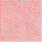
(b)

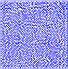
(c)

(d)

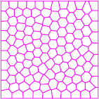
(e)

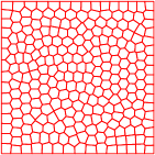
(f)

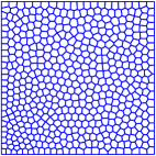
(g)

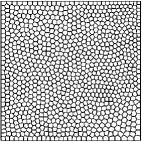
(h)

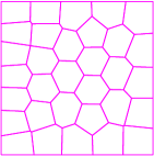
(i)

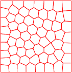
(j)

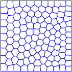
(k)

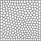
(l)

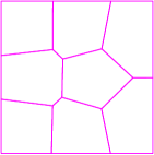
(m)

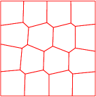
(n)

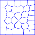
(o)

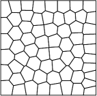
(p)

Figure 1: Sets of non-nested grids employed for numerical simulations.

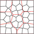
(a)

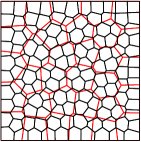
(b)

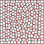
(c)

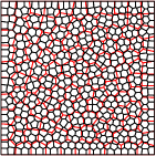
(d)

Figure 2: Example of non-nested partition.

In this section we present several numerical results to test the theoretical convergence estimates provided in Theorem 4.1. We focus on a two dimensional problem on the unit square $\Omega=(0,1)^{2}$. For the simulations, we consider the sets of polygonal grids shown in Figure 1. Each polygonal element mesh is generated through the Voronoi Diagram algorithm by using the software package PolyMesher Talietal12 . In particular the finest grids (Level 4) of Figure 1 consist of 512 (Set 1), 1024 (Set 2), 2048 (Set 3) and 4096 (Set 4) elements. Starting from the number of elements of each initial mesh, a sequence of coarse, non-nested partitions is generated: each coarse mesh is built independently from the finer one, with the only constrain that the number of element is approximately $1/4$ of the finer one. An example of sequence of non-nested partitions is shown in Figure 2.

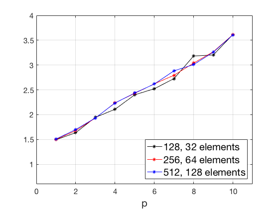
Figure 3: Estimates of $\mathsf{C}_{\mathsf{stab}}(p)$ in Lemma 6 as a function of $p$. Non-nested Voronoi meshes as shown in Figure 1.

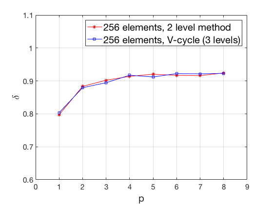
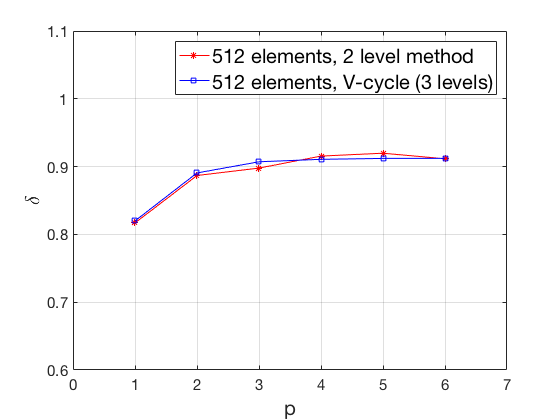
Figure 4: Estimates of $\delta_{2}$ and $\delta_{3}$ in Theorem 4.1 as a function of $p$, with $m_{1}=m_{2}=m=3p^{2}$ and two polyhedral grids of $256$ (left) and $512$ (right) elements.

First of all, we verify the estimate of Lemma 6, numerically evaluating $\mathsf{C}_{\mathsf{stab}}(p)\approx p$, where $p$ is the polynomial approximation degree. To this aim we consider three pairs of non-nested grids, where the number of elements of the coarser grid is the number of the finer divided by $4$: for each pair, we compute the value of $\mathsf{C}_{\mathsf{stab}}(p)$ as a function of $p$. Figure 3 show that, as expected, $\mathsf{C}_{\mathsf{stab}}(p)$ depends linearly on $p$ and is independent of the mesh-size $h$.

We now consider the grids shown in Set 1 and in Set 2 of Figure 1, and numerically evaluate the constant $\delta_{j}$ in Theorem 4.1 based on selecting the Richardson smoother with $m_{1}=m_{2}=m=3p^{2}$, cf. Figure 4. Here, we observe that $\delta_{2}$ and $\delta_{3}$ are asymptotically constant, as the polynomial degree $p$ increases showing that our two-level and V-cycle algorithms are uniformly convergent also with respect to $p$ provided that $m\approx p^{2}$.

Next, we investigate the performance of the iterative Multigrid non-nested V-cycle algorithm presented in Sect. 4. In order to do that, we solve the Poisson problem with homogeneous Dirichlet boundary conditions on the unit square $\Omega=(0,1)^{2}$, and we compute the number of iterations needed by our V-cycle algorithm to reduce the relative residual error below a given tolerance of $10^{-8}$, by varying the polynomial degree of approximation and the granularity of the finest grid. In Table 1 we report the convergence factors

$$\rho_{J}=\exp\left(\frac{1}{N_{it,J}}\ln\frac{\|\mathbf{r}_{N_{it,J}}\|}{\|\mathbf{r}_{0}\|}\right),$$ (83)

where $N_{it,J}$ is the iteration counts needed to attain convergence of the $h$-version of the V-cycle scheme with $J$ levels, where $J=2,3,4$, while $\mathbf{r}_{N_{it,J}}$ and $\mathbf{r}_{0}$ are the final and initial residual vectors, respectively. Here the polynomial approximation degree on each level is chosen as $p_{j}=1$, $j=1,\dots,J$, while we vary the number of elements of the finest grid and the number of smoothing steps ($m_{1}=m_{2}=m$). According to Theorem 4.1, the convergence factor is independent from the spatial discretization step $h$, indeed, for a fixed $J\in\{2,3,4\}$ ad a fixed number of pre-smoothing steps $m$, the convergence factor is roughly constant between the 4 sets of grids. In particular, this means that the number of iterations needed from the proposed V-cycle method to attain the convergence is not influenced by the mesh refinement, contrarily of what we observe for the Conjugate Gradient (CG) method. As expected, the convergence factor is reduced by increasing the number of smoothing step.

Table 1: Converge factors $\rho_{J}$ of V-cycle multigrid method as a function of $m$ and a comparison with the iteration counts of the CG method ($C_{\sigma}^{j}\equiv C_{\sigma}=10$, $p=1$).

	Set 1, $N_{iter}^{CG}=410$			Set 2, $N_{iter}^{CG}=600$
	2 levels	3 levels	4 levels	2 levels	3 levels	4 levels
$m=3$	0.77	0.83	0.83	0.82	0.84	0.85
$m=5$	0.69	0.76	0.78	0.74	0.77	0.79
$m=8$	0.63	0.69	0.72	0.66	0.70	0.73
	Set 3, $N_{iter}^{CG}=867$			Set 4, $N_{iter}^{CG}=1228$
	2 levels	3 levels	4 levels	2 levels	3 levels	4 levels
$m=3$	0.79	0.85	0.93	0.78	0.84	0.87
$m=5$	0.72	0.79	0.82	0.71	0.78	0.81
$m=8$	0.65	0.72	0.76	0.64	0.72	0.74

Table 2: Converge factors $\rho_{J}$ (and iterations count) of the V-cycle methods as a function of the number $m$ of pre-smoothing steps and comparison with the iteration counts of the CG method ($C_{\sigma}^{j}\equiv C_{\sigma}=10$, $p=3$).

	Set 1, $N_{iter}^{CG}=2212$			Set 2, $N_{iter}^{CG}=3223$
	2 levels	3 levels	4 levels	2 levels	3 levels	4 levels
$m=3$	0.99 (3306)	0.98 (992)	0.98 (955)	0.97 (616)	0.98 (852)	0.98 (1024)
$m=5$	0.96 (429)	0.97 (566)	0.97 (591)	0.95 (396)	0.96 (523)	0.97 (626)
$m=8$	0.94 (296)	0.95 (367)	0.95 (388)	0.94 (277)	0.95 (339)	0.95 (403)
	Set 3, $N_{iter}^{CG}=4174$			Set 4, $N_{iter}^{CG}=6689$
	2 levels	3 levels	4 levels	2 levels	3 levels	4 levels
$m=3$	-	0.98 (1061)	0.98 (860)	-	0.97 (699)	0.98 (823)
$m=5$	0.96 (428)	0.97 (648)	0.97 (527)	0.95 (392)	0.96 (435)	0.96 (508)
$m=8$	0.94 (288)	0.96 (418)	0.95 (341)	0.93 (273)	0.94 (290)	0.95 (335)

We have repeated the same set of experiments employing $p_{j}=3,\ \forall j=1,\dots,J$; the results are reported in Table 2, where we also have reported the iterations count (between parenthesis). Firstly, a comparison between Table 1 and Table 2 confirms that the convergence factor increases as $p$ grows up if the number of smoothing steps is kept fixed. Secondly, we observe that if the number of smoothing step is kept too small then the convergence of the method could not be guaranteed: indeed, according to Theorem 4.1, a uniformly convergent (also with respect to $p$) solver require a number of smoothing steps $m>2C_{1}C_{Q}\gtrsim p^{2+\mu}$ as shown in Figure 4. If $m$ is big enough, we observe that also in this case the number of iterations does not depend from the granularity of the underlying mesh, while the iterations count of the Conjugate Gradient method is growing if $h$ decrease.

6 Additive Schwarz smoother

In order to improve the convergence properties of the V-cycle algorithm studied above, we define in this section a domain decomposition preconditioner that we will use as a smoothing operator instead of the Richardson iteration. To this end, let $\mathcal{T}_{j}$ and $\mathcal{T}_{j-1}$ be respectively the finer and the coarser non-nested meshes, satisfying the grid assumptions given in Sect. 2.1. We then introduce the local and coarse solvers, that are the key ingredients in the definition of the smoother on the space $V_{j},\ j=2,\dots,J$.

Local Solvers. Let us consider the finest mesh $\mathcal{T}_{j}$ with cardinality $N_{j}$, then for each element $\kappa_{i}\in\mathcal{T}_{j}$, we define a local space $V_{j}^{i}$ as the restriction of the DG finite element space $V_{j}$ to the element $\kappa_{i}\in\mathcal{T}_{j}$:

$$V_{j}^{i}=V_{j}|_{\kappa_{i}}\equiv\mathcal{P}_{p_{j}}(\kappa_{i})\qquad\forall i=1,...,N_{j},$$ (84)

and for each local space, the associated local bilinear form is defined by

$$\mathcal{A}_{j}^{i}:V_{j}^{i}\times V_{j}^{i}\rightarrow\mathbb{R},\quad\mathcal{A}_{j}^{i}(u_{i},v_{i})=\mathcal{A}_{j}(R_{i}^{T}u_{i},R_{i}^{T}v_{i})\quad\forall u_{i},v_{i}\in V^{i},$$ (85)

where $R_{i}^{T}:V_{j}^{i}\rightarrow V_{j}$ denotes the classical extension by-zero operator from the local space $V_{j}^{i}$ to the global $V_{j}$.

Coarse Solver. The natural choice in our contest is to define the coarse space $V^{0}_{j}$ to be exactly the same used for the Coarse grid correction step of the V-cycle algorithm introduced in Sect. 4, that is

$$V^{0}_{j}=V_{j-1}\equiv\{v\in L^{2}(\Omega):v|_{\kappa}\in\mathcal{P}_{p_{j-1}}(\kappa),\kappa\in\mathcal{T}_{j-1}\},$$ (86)

the bilinear form on $V^{0}_{j}$ is then given by

$$\mathcal{A}_{j}^{0}:V_{j}^{0}\times V_{j}^{0}\rightarrow\mathbb{R},\quad\mathcal{A}_{j}^{0}(u_{0},v_{0})=\mathcal{A}_{j-1}(u_{0},v_{0})\quad\forall u_{0},v_{0}\in V_{j}^{0}.$$ (87)

We also define the injection operator from $V_{j}^{0}$ to $V_{j}$: conversely with respect to the case where the coarser mesh is obtained by agglomeration, here the injection operator is not trivial, and it is defined as the prolongation operator introduced in Sect. 4, that is $R_{0}^{T}:V_{j}^{0}\rightarrow V_{j},\ R_{0}^{T}=I_{j-1}^{j}.$ By introducing the projection operators $P_{i}=R_{i}^{T}\tilde{P_{i}}:V_{j}\rightarrow V_{j},\text{ }i=0,1,\dots,N_{j},$ where

$$\tilde{P_{i}}:V_{j}\rightarrow V^{i}_{j},\quad\mathcal{A}_{j}^{i}(\tilde{P_{i}}v_{h},w_{i})=\mathcal{A}_{j}(v_{h},R_{i}^{T}w_{i})\quad\forall w_{i}\in V^{i}_{j},\quad i=1,\dots,N_{j},$$ (88)

$$\tilde{P_{0}}:V_{j}\rightarrow V^{0}_{j},\quad\mathcal{A}_{j}^{0}(\tilde{P_{0}}v_{h},w_{0})=\mathcal{A}_{j}(v_{h},R_{0}^{T}w_{0})\quad\forall w_{0}\in V^{0}_{j},$$ (89)

the additive Schwarz operator is defined by $P_{ad}=\sum_{i=0}^{N_{j}}(R_{i}^{T}(A^{i}_{j})^{-1}R_{i})A_{j}\equiv B^{-1}_{ad}A_{j},$ where $B^{-1}_{ad}=\sum_{i=0}^{N_{j}}(R_{i}^{T}(A^{i}_{j})^{-1}R_{i})$ is the preconditioner. Then, the Additive Schwarz smoothing operator with $m$ steps consists in performing $m$ iterations of the Preconditioned Conjugate Gradient method using $B_{ad}$ as preconditioner. In Algorithm 3 we outline the V-cycle multigrid method using $P_{ad}$ as a smoother. Here, $\mathsf{MG_{\mathcal{AS}}}(j,g,z_{0},m_{1},m_{2})$ denotes the approximate solution of $A_{j}z=g$ obtained after one iteration, with initial guess $z_{0}$ and $m_{1}$, $m_{2}$ pre- and post-smoothing steps, respectively. Here, the smoothing step is performed by the algorithm $ASPCG$, i.e., $z=ASPCG(A,z_{0},g,m)$ represents the output of $m$ steps of Preconditioned Conjugate Gradient method applied to the linear system of equations $Ax=g,$ by using $B_{as}$ as preconditioner and starting with the initial guess $z_{0}$.

Algorithm 3 One iteration of Multigrid V-cycle scheme with AS-smoother

Pre-smoothing:

if j=1 then

     $\mathsf{MG}_{\mathcal{AS}}(1,g,z_{0},m_{1},m_{2})=A_{1}^{-1}g.$

else

     Pre-smoothing:

     $z^{(m_{1})}=ASPCG(A_{j},z_{0},g,m_{1})$;

     Coarse grid correction:

     $r_{j-1}=I_{j}^{j-1}(g-A_{j}z^{(m_{1})})$;

     $e_{j-1}=\mathsf{MG}_{\mathcal{AS}}(j-1,r_{j-1},0,m_{1},m_{2})$;

     $z^{(m_{1}+1)}=z^{(m_{1})}+I_{j-1}^{j}e_{j-1}$;

     Post-smoothing:

     $z^{(m_{1}+m_{1}+1)}=ASPCG(A_{j},z^{(m_{1}+1)},g,m_{2});$

     $\mathsf{MG}_{\mathcal{AS}}(j,g,z_{0},m_{1},m_{2})=z^{(m_{1}+m_{2}+1)}.$

end if

The numerical performance of Algorithm 3 are reported in Tables 3, 4 and 5, for the corresponding V-cycle algorithm with $J=2,3,4$ levels. The simulations are similar to the ones described in the previous section: here we used the grids of Set 2, 3 and 4 of Figure 1, and we varied the polynomial degree $p\in\{1,3,5\}$. Firstly, we observe that, also in this case, the number of iteration does not increase with the number of elements in the underlying mesh for a fixed number of smoothing steps $m$; moreover, we does not observe the constrain from below required to the number of smoothing steps with respect to the degree of approximation: the method converges also with high degree of approximation and a small number of smoothing steps. Finally, Table 6 shows the numerical results relatives to an example of $hp$-multigrid, characterized by a choice of different polynomial degrees of approximation between non-nested space: also in this case we observe that the number of iterations is independent of the granularity of the finest mesh, and we have convergence for any choice of smoothing steps $m$.

Table 3: Iteration counts of the V-cycle solvers with the Additive Schwarz smoother as a function of $m$ ($C_{\sigma}^{j}\equiv C_{\sigma}=10$, $p=1$).

	Set 2			Set 3			Set 4
	2 lev.	3 lev.	4 lev.	2 lev.	3 lev.	4 lev.	2 lev.	3 lev.	4 lev.
$m=3$	18	18	18	18	18	18	20	20	20
$m=5$	9	9	9	9	9	9	10	10	10
$m=8$	5	5	5	5	5	5	5	5	5
	$N_{iter}^{CG}=600$			$N_{iter}^{CG}=867$			$N_{iter}^{CG}=1228$

Table 4: Iteration counts of the V-cycle solvers with the Additive Schwarz smoother as a function of $m$ ($C_{\sigma}^{j}\equiv C_{\sigma}=10$, $p=3$).

	Set 2			Set 3			Set 4
	2 lev.	3 lev.	4 lev.	2 lev.	3 lev.	4 lev.	2 lev.	3 lev.	4 lev.
$m=3$	63	64	64	57	59	59	59	60	60
$m=5$	27	27	27	25	25	25	26	26	26
$m=8$	13	13	13	13	14	14	14	14	14
	$N_{iter}^{CG}=3223$			$N_{iter}^{CG}=4174$			$N_{iter}^{CG}=6689$

Table 5: Iteration counts of the V-cycle solvers with the Additive Schwarz smoother as a function of $m$ ($C_{\sigma}^{j}\equiv C_{\sigma}=10$, $p=5$).

	Set 2			Set 3			Set 4
	2 lev.	3 lev.	4 lev.	2 lev.	3 lev.	4 lev.	2 lev.	3 lev.	4 lev.
$m=3$	148	156	156	125	132	132	149	158	157
$m=5$	59	59	58	51	51	51	59	60	60
$m=8$	26	26	26	24	24	24	27	27	27
	$N_{iter}^{CG}=7676$			$N_{iter}^{CG}=11525$			$N_{iter}^{CG}=15814$

Table 6: Iteration counts of the $hp$-version of the V-cycle solvers with the Additive Schwarz smoother as a function of $m$. Here the polynomial degree on each space is $p_{j}=j$ for $j=1,2,3,4$.

	Set 2			Set 3			Set 4
	2 lev.	3 lev.	4 lev.	2 lev.	3 lev.	4 lev.	2 lev.	3 lev.	4 lev.
$m=3$	85	86	86	79	80	80	83	85	84
$m=5$	35	35	35	32	32	32	33	33	33
$m=8$	17	17	17	17	17	17	17	18	17
	$N_{iter}^{CG}=5108$			$N_{iter}^{CG}=7697$			$N_{iter}^{CG}=10572$

Appendix A Proof of Lemma 1

Proof (of Lemma 1)

We follow the idea of (DiPiEr, , Proof of Lemma 1.49). First of all, we observe that

$$\|v\|_{L^{2}(\partial\kappa)}^{2}=\sum_{F\subset\partial\kappa}\|v\|_{L^{2}(F)}^{2}.$$ (90)

For each face $F\subset\partial\kappa$ let $T_{F}\subset\kappa$ be a $d$-dimensional simplex sharing the face $F$ with $\kappa$ and satisfying the Assumption 2.1: in $T_{F}$ we define a function $\sigma_{F}$ as follow:

$$\sigma_{F}:\textbf{x}\in\overline{T_{F}}\mapsto\sigma_{F}(\textbf{x})=\frac{|F|}{d|T_{F}|}(\textbf{x}-\textbf{v}_{F}),$$ (91)

where $\textbf{v}_{F}$ is the vertex of the simplex $T_{F}$ opposite to the face $F$. We observe that:

• $\sigma_{F}(\textbf{x})\cdot\textbf{n}_{F}=\frac{|F|}{d|T_{F}|}\tilde{h}\ \forall\textbf{x}\in F$, where $\tilde{h}$ is the height of the simplex respect to the face $F$, that is also $\tilde{h}=\frac{d|T_{F}|}{|F|}$, then $\sigma_{F}|_{F}\cdot\textbf{n}_{F}=1$;

• $\sigma_{F}|_{F^{\prime}}\cdot\textbf{n}_{F^{\prime}}=0\ \forall\text{ faces }F^{\prime}\subset\partial T_{F},F^{\prime}\neq F$;

then we have:

$$\|v\|_{L^{2}(F)}^{2} =\int_{F}|v|^{2}d\sigma=\int_{\partial T_{F}}|v|^{2}\sigma_{F}\cdot\textbf{n}_{F}d\sigma=\int_{T}\nabla\cdot(|v|^{2}\sigma_{F})d\textbf{x}$$ (92)

$$=\int_{T}2v\nabla v\cdot\sigma_{F}d\textbf{x}+\int_{T}|v|^{2}\nabla\cdot\sigma_{F}d\textbf{x};$$ (93)

now the following properties hold for $\sigma_{F}$:

• $\nabla\cdot\sigma_{F}=\nabla\cdot\frac{|F|}{d|T_{F}|}(\textbf{x}-\textbf{v}_{F})=\frac{|F|}{d|T_{F}|}\nabla\cdot\textbf{x}=\frac{|F|}{|T_{F}|}$;

• $\|\sigma_{F}\|_{[L^{\infty}(T_{F})]^{d}}=\frac{|F|}{d|T_{F}|}h_{T}\leq\frac{|F|}{d|T_{F}|}h_{\kappa}$,

which implies:

$$\|v\|_{L^{2}(F)}^{2} \leq 2\|\sigma_{F}\|_{[L^{\infty}(T_{F})]^{d}}\|v\nabla v\|_{[L^{1}(T_{F})]^{d}}+\frac{|F|}{|T_{F}|}\|v\|_{L^{2}(T_{F})}^{2},$$ (94)

$$\leq 2\frac{|F|}{d|T_{F}|}h_{\kappa}\|v\|_{L^{2}(T_{F})}|v|_{H^{1}(T_{F})}+\frac{|F|}{|T_{F}|}\|v\|_{L^{2}(T_{F})}^{2},$$ (95)

using the Assumption 2.1 we have

$$\|v\|_{L^{2}(F)}^{2}\leq 2C\|v\|_{L^{2}(T_{F})}|v|_{H^{1}(T_{F})}+\frac{Cd}{h_{\kappa}}\|v\|_{L^{2}(T_{F})}^{2}.$$ (96)

By using Young Inequality we could bound

$$\|v\|_{L^{2}(T_{F})}|v|_{H^{1}(T_{F})}\leq\frac{1}{2}\Bigl{(}\frac{\epsilon}{h_{\kappa}}\|v\|_{L^{2}(T_{F})}^{2}+\frac{h_{\kappa}}{\epsilon}|v|_{H^{1}(T_{F})}^{2}\Bigr{)},$$ (97)

where we have chosen $\epsilon\geq 1$. Using the previous inequality we have

$$\|v\|_{L^{2}(F)}^{2}\leq 2Cd\Bigl{(}\frac{\epsilon}{h_{\kappa}}\|v\|_{L^{2}(T_{F})}^{2}+\frac{h_{\kappa}}{\epsilon}|v|_{H^{1}(T_{F})}^{2}\Bigr{)}.$$ (98)

we observe that (98) holds $\forall F\subset\partial\kappa$. Then, thanks to (90), we have

$$\|v\|_{L^{2}(\partial\kappa)}^{2} =\sum_{F\subset\partial\kappa}\|v\|_{L^{2}(F)}^{2}\leq\sum_{F\subset\partial\kappa}2Cd\Bigl{(}\frac{\epsilon}{h_{\kappa}}\|v\|_{L^{2}(T_{F})}^{2}+\frac{h_{\kappa}}{\epsilon}|v|_{H^{1}(T_{F})}^{2}\Bigr{)}$$ (99)

$$=2Cd\Bigl{(}\frac{\epsilon}{h_{\kappa}}\sum_{F\subset\partial\kappa}\|v\|_{L^{2}(T_{F})}^{2}+\frac{h_{\kappa}}{\epsilon}\sum_{F\subset\partial\kappa}|v|_{H^{1}(T_{F})}^{2}\Bigr{)}$$ (100)

$$\leq 2Cd\Bigl{(}\frac{\epsilon}{h_{\kappa}}\|v\|_{L^{2}(\kappa)}^{2}+\frac{h_{\kappa}}{\epsilon}|v|_{H^{1}(\kappa)}^{2}\Bigr{)},$$ (101)

where in the last inequality we have used the fact that the simplices of the set $\{T_{F}:F\subset\partial\kappa\}$ satisfy Assumption 2.1, in the sense that they are disjoints and $\cup_{F\subset\partial\kappa}\overline{T_{F}}\subset\overline{\kappa}$.

Appendix B Proof of Lemma 7

In order to show Lemma 7 we follow the analysis presented in DuanGaoTanZhang , by firstly showing two preliminary results making use of the properties presented in Sect. 3.

Lemma 8

Let Assumptions 2.1 - 2.4 hold, and let $\widetilde{\Pi}_{j}$ be the projection operator on $V_{j}$ as defined in Lemma 4, for $j=J,J-1$. Then

$$\|\widetilde{\Pi}_{J}w-I_{J-1}^{J}\widetilde{\Pi}_{J-1}w\|_{L^{2}(\Omega)}\lesssim\frac{h_{J}^{2}}{p_{J}^{2}}\|w\|_{H^{2}(\Omega)}\quad\forall w\in H^{2}(\Omega).$$ (102)

Proof

Using the triangular inequality, Remark 6 and the approximation estimates of Lemma 4 we have:

$$\|\widetilde{\Pi}_{J}w-I_{J-1}^{J} \widetilde{\Pi}_{J-1}w\|_{L^{2}(\Omega)}\leq$$ (103)

$$\leq\|\widetilde{\Pi}_{J}w-w\|_{L^{2}(\Omega)}+\|w-Q_{J}w\|_{L^{2}(\Omega)}+\|Q_{J}w-I_{J-1}^{J}\widetilde{\Pi}_{J-1}w\|_{L^{2}(\Omega)}$$ (104)

$$=\|\widetilde{\Pi}_{J}w-w\|_{L^{2}(\Omega)}+\min_{z_{h}\in V_{J}}\|w-z_{h}\|_{L^{2}(\Omega)}+\|Q_{J}(w-\widetilde{\Pi}_{J-1}w)\|_{L^{2}(\Omega)}$$ (105)

$$\leq\|\widetilde{\Pi}_{J}w-w\|_{L^{2}(\Omega)}+\|\ w-\widetilde{\Pi}_{J}w\|_{L^{2}(\Omega)}+\|w-\widetilde{\Pi}_{J-1}w\|_{L^{2}(\Omega)}$$ (106)

$$\lesssim\frac{h_{J}^{2}}{p_{J}^{2}}\|w\|_{H^{2}(\Omega)}+\frac{h_{J-1}^{2}}{p_{J-1}^{2}}\|w\|_{H^{2}(\Omega)}\lesssim\frac{h_{J}^{2}}{p_{J}^{2}}\|w\|_{H^{2}(\Omega)},$$ (107)

where in the last inequality we also used hypothesis (4) and (5).

Lemma 9

Let Assumptions 2.1 - 2.4 hold. Let be $g\in L^{2}(\Omega)$ and denote by $w_{j}\in V_{j}$ the solution of $\mathcal{A}_{j}(w_{j},v)=(g,v)_{L^{2}(\Omega)}$ $\forall v\in V_{j}$ with $j=J-1,J$. Then the following inequality holds:

$$\|w_{J}-I_{J-1}^{J}w_{J-1}\|_{L^{2}(\Omega)}+\|w_{J-1}-P_{J}^{J-1}w_{J}\|_{L^{2}(\Omega)}\lesssim\frac{h_{J}^{2}}{p_{J}^{2-\mu}}\|g\|_{L^{2}(\Omega)}.$$ (108)

Proof

Consider the unique solution $w\in V$ of the problem

$$\mathcal{A}(w,v)=(g,v)_{L^{2}(\Omega)}\quad\forall v\in V.$$ (109)

Using Theorem 3.1 we have

$$\|w-w_{j}\|_{L^{2}(\Omega)}\lesssim\frac{h_{j}^{2}}{p_{j}^{2-\mu}}\|w\|_{L^{2}(\Omega)},\quad j=J-1,J.$$ (110)

Using the triangular inequality and Remark 6 we have:

$$\|w_{J}-I_{J-1}^{J}w_{J-1} \|_{L^{2}(\Omega)}\leq\|w_{J}-w\|_{L^{2}(\Omega)}+\|w-\widetilde{\Pi}_{J}w\|_{L^{2}(\Omega)}$$ (111)

$$\quad+\|\widetilde{\Pi}_{J}w-I_{J-1}^{J}\widetilde{\Pi}_{J-1}w\|_{L^{2}(\Omega)}+\|I_{J-1}^{J}\widetilde{\Pi}_{J-1}w-Q_{J}w\|_{L^{2}(\Omega)}$$ (112)

$$\quad+\|Q_{J}w-I_{J-1}^{J}w_{J-1}\|_{L^{2}(\Omega)}$$ (113)

$$=\|w_{J}-w\|_{L^{2}(\Omega)}+\|w-\widetilde{\Pi}_{J}w\|_{L^{2}(\Omega)}+\|\widetilde{\Pi}_{J}w-I_{J-1}^{J}\widetilde{\Pi}_{J-1}w\|_{L^{2}(\Omega)}$$ (114)

$$\quad+\|Q_{J}(\widetilde{\Pi}_{J-1}w-w)\|_{L^{2}(\Omega)}+\|Q_{J}(w-w_{J-1})\|_{L^{2}(\Omega)}$$ (115)

$$\leq\|w_{J}-w\|_{L^{2}(\Omega)}+\|w-\widetilde{\Pi}_{J}w\|_{L^{2}(\Omega)}+\|\widetilde{\Pi}_{J}w-I_{J-1}^{J}\widetilde{\Pi}_{J-1}w\|_{L^{2}(\Omega)}$$ (116)

$$\quad+\|\widetilde{\Pi}_{J-1}w-w\|_{L^{2}(\Omega)}+\|w-w_{J-1}\|_{L^{2}(\Omega)}.$$ (117)

Using (110), Lemma 4 and Lemma 8, we have

$$\|w_{J}-I_{J-1}^{J}w_{J-1}\|_{L^{2}(\Omega)} \lesssim\frac{h_{J}^{2}}{p_{J}^{2-\mu}}\|w\|_{H^{2}(\Omega)}+\frac{h_{J}^{2}}{p_{J}^{2}}\|w\|_{H^{2}(\Omega)}+\frac{h_{J}^{2}}{p_{J}^{2}}\|w\|_{H^{2}(\Omega)}$$ (118)

$$\quad+\frac{h_{J-1}^{2}}{p_{J-1}^{2}}\|w\|_{H^{2}(\Omega)}+\frac{h_{J-1}^{2}}{p_{J-1}^{2-\mu}}\|w\|_{H^{2}(\Omega)}.$$ (119)

From the elliptic regularity assumption (2) and hypothesis (4) and (5), we can write

$$\|w_{J}-I_{J-1}^{J}w_{J-1}\|_{L^{2}(\Omega)}\lesssim\frac{h_{J}^{2}}{p_{J}^{2-\mu}}\|g\|_{L^{2}(\Omega)}.$$ (120)

Now, let $z_{j}\in V_{j}$ be the solution of:

$$\mathcal{A}_{j}(z_{j},q)=(w_{J-1}-P_{J}^{J-1}w_{J},q_{j})_{L^{2}(\Omega)}\quad\forall q_{j}\in V_{j},\quad j=J-1,J;$$ (121)

Using (120) we get the following estimate:

$$\|z_{J-1}-I_{J-1}^{J}z_{J-1}\|_{L^{2}(\Omega)}\lesssim\frac{h_{J}^{2}}{p_{J}^{2-\mu}}\|w_{J-1}-P_{J}^{J-1}w_{J}\|_{L^{2}(\Omega)}.$$ (122)

Then, we have:

$$\|w_{J-1}-P_{J}^{J-1}w_{J}\|_{L^{2}(\Omega)}^{2} =\mathcal{A}_{J-1}(z_{J-1},w_{J-1}-P_{J}^{J-1}w_{J})$$ (123)

$$=\mathcal{A}_{J-1}(z_{J-1},w_{J-1})-\mathcal{A}_{J}(I_{J-1}^{J}z_{J-1},w_{J})$$ (124)

$$=(z_{J-1},g)-(I_{J-1}^{J}z_{J-1},g)=(g,z_{J-1}-I_{J-1}^{J}z_{J-1})$$ (125)

$$\lesssim\|g\|_{L^{2}(\Omega)}\frac{h_{J}^{2}}{p_{J}^{2-\mu}}\|w_{J-1}-P_{J}^{J-1}w_{J}\|_{L^{2}(\Omega)},$$ (126)

from which, together with (120), inequality (108) follows.

Proof (of Lemma 7)

For any $v_{J}\in V_{J}$ we consider the following equality:

$$\|(\textnormal{Id}_{J}-I_{J-1}^{J}P_{J}^{J-1})v_{J}\|_{L^{2}(\Omega)}=\sup_{0\neq\phi\in L^{2}(\Omega)}\frac{\bigl{(}\phi,(\textnormal{Id}_{J}-I_{J-1}^{J}P_{J}^{J-1})v_{J}\bigl{)}_{L^{2}(\Omega)}}{\|\phi\|_{L^{2}(\Omega)}missing}.$$ (127)

Next, consider the solution $z_{j}$ of the following problems

$$\mathcal{A}_{j}(z_{j},v_{j})=\bigl{(}\phi,v_{j}\bigr{)}\quad\forall v_{j}\in V_{j},\text{ for }j=J,J-1.$$ (128)

By using the definition of $P_{J}^{J-1}$ and Lemma 9, we have:

$$\bigl{(}\phi,(\textnormal{Id}_{J}-I_{J-1}^{J} P_{J}^{J-1})v_{J})\bigr{)}_{L^{2}(\Omega)}=\mathcal{A}_{J}(z_{J},v_{J})-\mathcal{A}_{J-1}(P_{J}^{J-1}z_{J},P_{J}^{J-1}v_{J})$$ (129)

$$=\mathcal{A}_{J}(z_{J}-I_{J-1}^{J}z_{J-1},v_{J})+\mathcal{A}_{J}(I_{J-1}^{J}(z_{J-1}-P_{J}^{J-1}z_{J}),v_{J})$$ (130)

$$\leq|\mathchoice{{}\mkern-3.0mu}{{}\mkern-3.0mu}{{}\mkern-3.0mu}{}|\mathchoice{{}\mkern-3.0mu}{{}\mkern-3.0mu}{{}\mkern-3.0mu}{}|v_{J}|\mathchoice{{}\mkern-3.0mu}{{}\mkern-3.0mu}{{}\mkern-3.0mu}{}|\mathchoice{{}\mkern-3.0mu}{{}\mkern-3.0mu}{{}\mkern-3.0mu}{}|_{2,J}\Bigl{(}\|z_{J}-I_{J-1}^{J}z_{J-1}\|_{L^{2}(\Omega)}+\|z_{J-1}-P_{J}^{J-1}z_{J}\|_{L^{2}(\Omega)}\Bigr{)}$$ (131)

$$\lesssim|\mathchoice{{}\mkern-3.0mu}{{}\mkern-3.0mu}{{}\mkern-3.0mu}{}|\mathchoice{{}\mkern-3.0mu}{{}\mkern-3.0mu}{{}\mkern-3.0mu}{}|v_{J}|\mathchoice{{}\mkern-3.0mu}{{}\mkern-3.0mu}{{}\mkern-3.0mu}{}|\mathchoice{{}\mkern-3.0mu}{{}\mkern-3.0mu}{{}\mkern-3.0mu}{}|_{2,J}\frac{h_{J}^{2}}{p_{J}^{2-\mu}}\|\phi\|_{L^{2}(\Omega)}.$$ (132)

Using the last inequality together with (127) we get (74).

References

• (1) Antonietti, P.F., Brezzi, F., Marini, L.D.: Stabilizations of the Baumann-Oden DG formulation: the 3D case. Boll. Unione Mat. Ital. 1(3), 629 – 643 (2008)
• (2) Antonietti, P.F., Facciolà, C., Russo, A., Verani, M.: Discontinuous Galerkin approximation of flows in fractured porous media. Technical Report 22/2016, MOX Report (2016)
• (3) Antonietti, P.F., Giani, S., Houston, P.: $hp$-version composite Discontinuous Galerkin methods for elliptic problems on complicated domains. SIAM J. Sci. Comput. 35(3), A1417 – A1439 (2013)
• (4) Antonietti, P.F., Giani, S., Houston, P.: Domain decomposition preconditioners for Discontinuous Galerkin methods for elliptic problems on complicated domains. J. Sci. Comput. 60(1), 203–227 (2014)
• (5) Antonietti, P.F., Houston, P.: A class of domain decomposition preconditioners for $hp$-Discontinuous Galerkin finite element methods. J. Sci. Comput. 46(1), 124 – 149 (2011)
• (6) Antonietti, P.F., Houston, P., Hu, X., Sarti, M., Verani, M.: Multigrid algorithms for $hp$-version Interior Penalty Discontinuous Galerkin methods on polygonal and polyhedral meshes. Calcolo pp. 1 – 30 (2017)
• (7) Antonietti, P.F., Houston, P., Smears, I.: A note on optimal spectral bounds for nonoverlapping domain decomposition preconditioners for $hp$-version Discontinuous Galerkin methods. Internat. J. Numer. Methods Engrg. 13(4), 513–524 (2016)
• (8) Antonietti, P.F., Mazzieri, I.: DG methods for the elastodynamics equations on polygonal/polyhedral grids. in praparation (2017)
• (9) Antonietti, P.F., Sarti, M., Verani, M.: Multigrid algorithms for $hp$-Discontinuous Galerkin discretizations of elliptic problems. SIAM J. Numer. Anal. 53(1), 598 – 618 (2015)
• (10) Arnold, D.N.: An Interior Penalty Finite Element method with discontinuous elements. SIAM J. Numer. Anal. 19(4), 742 – 760 (1982)
• (11) Arnold, N.D., Brezzi, F., Cockburn, B., Marini, L.D.: Unified analysis of Discontinuous Galerkin methods for elliptic problems. SIAM J. Numer. Anal. 39(5), 1749 – 1779 (2002)
• (12) Baker, G.A.: Finite element methods for elliptic equations using nonconforming elements. Math. Comp. 31(137), 45 – 59 (1977)
• (13) Bank, R.E., Dupont, T.: An optimal order process for solving finite element equations. Math. Comp. 36(153), 35 – 51 (1981)
• (14) Bassi, F., Botti, L., Colombo, A., Brezzi, F., Manzini, G.: Agglomeration-based physical frame dG discretizations: an attempt to be mesh free. Math. Models Methods Appl. Sci. 24(8), 1495–1539 (2014)
• (15) Bassi, F., Botti, L., Colombo, A., Di Pietro, D.A., Tesini, P.: On the flexibility of agglomeration based physical space discontinuous Galerkin discretizations. J. Comput. Phys. 231(1), 45–65 (2012)
• (16) Bassi, F., Botti, L., Colombo, A., Rebay, S.: Agglomeration based Discontinuous Galerkin discretization of the Euler and Navier-Stokes equations. Comput. & Fluids 61, 77–85 (2012)
• (17) Braess, D., Verfürth, R.: Multigrid methods for nonconforming finite element methods. SIAM J. Numer. Anal. 22(4), 979 – 986 (1990)
• (18) Bramble, J.H.: Multigrid Methods (Pitman Research Notes in Mathematics Series). Longman Scientific and Technical (1993)
• (19) Bramble, J.H., Kwak, D.Y., Pasciak, J.E.: Uniform convergence of multigrid V-cycle iterations for indefinite and nonsymmetric problems. SIAM J. Numer. Anal. 31(6), 1746 – 1763 (1994)
• (20) Bramble, J.H., Pasciak, J.E.: The analysis of smoothers for multigrid algorithms. Math. Comp. 58(198), 467 – 488 (1992)
• (21) Bramble, J.H., Pasciak, J.E.: New estimates for multilevel algorithms including the V-cycle. Math. Comp. 60(202), 447 – 471 (1993)
• (22) Bramble, J.H., Pasciak, J.E.: Uniform convergence estimates for multigrid V-cycle algorithms with less than full elliptic regularity. SIAM J. Numer. Anal. 31(6), 1746 – 1763 (1994)
• (23) Bramble, J.H., Pasciak, J.E., Xu, J.: The analysis of multigrid algorithms with nonnested space or noninherited quadratic forms. Math. Comp. 56(193), 1–34 (1991)
• (24) Bramble, J.H., Zhang, X.: Uniform convergence of the multigrid V-cycle for an anisotropic problem. Math. Comp. 70(234), 453 – 470 (2001)
• (25) Cangiani, A., Dong, Z., Georgoulis, E.H.: $hp$-Version space-time Discontinuous Galerkin methods for parabolic problems on prismatic meshes. SIAM J. Sci. Comput. 39(4), A1251 – A1279 (2017)
• (26) Cangiani, A., Dong, Z., Georgoulis, E.H., Houston, P.: $hp$-Version Discontinuous Galerkin methods for advection-diffusion-reaction problems on polytopic meshes. ESAIM Math. Model. Numer. Anal. 50(3), 699 – 725 (2016)
• (27) Cangiani, A., Georgoulis, E.H., Houston, P.: $hp$-Version discontinuous Galerkin methods on polygonal and polyhedral meshes. Math. Models Methods Appl. Sci. 24(10), 2009 – 2041 (2014)
• (28) Cockburn, B., Karniadakis, G.E., Shu, C.W.: Discontinuous Galerkin Methods. Theory, computation and applications. Springer Berlin (2000)
• (29) Di Pietro, D.A., Ern, A.: Mathematical aspects of discontinuous Galerkin methods. Springer Science & Business Media (2011)
• (30) Duan, H.Y., Gao, S.Q., Tan, R.C.E., Zhang, S.: A generalized BPX multigrid framework covering nonnested V-cycle methods. Math. Comp. 76(257), 137–152 (2007)
• (31) Georgoulis, E.H., Suli, E.: Optimal error estimates for the $hp$-version Interior Penalty Discontinuous Galerkin finite element method. IMA J. Numer. Anal. 25(1), 205–220 (2005)
• (32) Giani, S., Houston, P.: Domain decomposition preconditioners for Discontinuous Galerkin discretizations of compressible fluid flows. Numer. Math. Theory Methods Appl. 7(2), 123 – 148 (2014)
• (33) Giani, S., Houston, P.: $hp$-Adaptive composite Discontinuous Galerkin methods for elliptic problems on complicated domains. Numer. Methods Partial Differential Equations 30(4), 1342 – 1367 (2014)
• (34) Gopalakrishnan, J., Kanschat, G.: Application of unified DG analysis to preconditioning DG methods. In: K.J. Bathe (ed.) Computational Fluid and Solid Mechanics 2003, pp. 1943 – 1945. Elsevier Science (2003)
• (35) Gopalakrishnan, J., Kanschat, G.: A multilevel Discontinuous Galerkin method. Numer. Math. 95(3), 527 – 550 (2003)
• (36) Gopalakrishnan, J., Pasciak, J.E.: Multigrid for the Mortar finite element method. SIAM J. Numer. Anal. 37(3), 1029 – 1052 (2000)
• (37) Hesthaven, J.S., Warburton, T.: Nodal Discontinuous Galerkin Methods: Algorithms, Analysis, and Applications, 1st edn. Springer Berlin (2008)
• (38) Lipnikov, K., Vassilev, D., Yotov, I.: Discontinuous Galerkin and mimetic finite difference methods for coupled Stokes-Darcy flows on polygonal and polyhedral grids. Numer. Math. 126(2), 321 – 360 (2014)
• (39) Monk, P., Zhang, S.: Multigrid computation of vector potentials. J. Comput. Appl. Math. 62(3), 301 – 320 (1995)
• (40) Nitsche, J.: Über ein Variationsprinzip zur Lösung von Dirichlet Problemen bei Verwendung von Teilräumen, die keinen Randbedingungen unterworfen sind. Abh. Math. Semin. Univ. Hambg. 36, 9 – 15 (1971)
• (41) Reed, W., Hill, T.: Triangular mesh methods for the neutron transport equation. Tech. Rep. LA-UR-73-479, Los Alamos Scientific Laboratory (1973)
• (42) Rivière, B.: Discontinuous Galerkin methods for solving elliptic and parabolic equations. SIAM (2008)
• (43) Scott, L.R., Zhang, S.: Higher-dimensional nonnested multigrid methods. Math. Comp. 58(198), 457 – 466 (1992)
• (44) Talischi, C., Paulino, G., Pereira, A., Menezes, I.: Polymesher: A general-purpose mesh generator for polygonal elements written in matlab. Struct. Multidiscip. Optim. 45(3), 309–328 (2012)
• (45) Wheeler, M.F.: An elliptic collocation Finite Element method with Interior Penalties. SIAM J. Numer. Anal. 15(1), 152 – 161 (1978)
• (46) Wiresaet, D., Kubatko, E.J., Michoski, C.E., Tanaka, S., Westerink, J.J., Dawson, C.: Discontinuous Galerkin methods with nodal and hybrid modal/nodal triangular, quadrilateral, and polygonal elements for nonlinear shallow water flow. Comput. Methods Appl. Mech. Engrg. 270, 113 – 149 (2014)
• (47) Xu, X., Chen, J.: Multigrid for the mortar element method for P1 nonconforming element. Numer. Math. 88(2), 381 – 389 (2001)
• (48) Xu, X., Li, L., Chen, W.: A multigrid method for the Mortar-type Morley element approximation of a plate bending problem. SIAM J. Numer. Anal. 39(5), 1712 – 1731 (2002)
• (49) Zhang, S.: Optimal-order nonnested multigrid methods for solving Finite Element equations I: on quasi-uniform meshes. Math. Comp. 55(191), 23 – 36 (1990)
• (50) Zhang, S., Zhang, Z.: Treatments of discontinuity and bubble functions in the multigrid method. Math. Comp. 66(219), 1055 – 1072 (1997)