Thin-shell wormholes from compact stellar objects

Abstract

This paper introduces a new type of thin-shell wormhole constructed from a special class of compact stellar objects rather than black holes. The construction and concomitant investigation of the stability to linearized radial perturbations commences with an extended version of a regular Hayward black hole. Given the equation of state $\mathcal{P}=\omega\sigma$, $\omega<0$, for the exotic matter on the thin shell, it is shown that whenever the value of the Hayward parameter is below its critical value, no stable solutions can exist. If the Hayward parameter is allowed to exceed its critical value, stable solutions can be found for moderately sized thin shells. Not only are the underlying structures ordinary compact objects, rather than black holes, the results are consistent with the properties of neutron stars, as well as other compact stellar objects.

Keywords: thin-shell wormholes; compact stellar objects; Hayward black holes

1 Introduction

A highly effective method for describing or mathematically constructing a class of spherically symmetric wormholes using the now standard cut-and-paste technique was proposed by Visser in 1989 [1]. The construction calls for grafting two black-hole spacetimes together, resulting in a thin-shell wormhole. By starting with a regular Hayward black hole, it is proposed in this paper that the construction can be extended to massive compact objects.

Apart from a number of forerunners, the concept of a traversable wormhole suitable for interstellar travel was first proposed by Morris and Thorne [2]. It turned out that a wormhole could only be held open by violating the null energy condition, defined as follows:

$$T_{\alpha\beta}k^{\alpha}k^{\beta}\geq 0$$ (1)

for all null vectors $k^{\alpha}$. Matter that violates this condition came to be called “exotic.” In particular, for the radial outgoing null vector $(1,1,0,0)$, the violation takes on the form $T_{\alpha\beta}k^{\alpha}k^{\beta}=\rho+p<0$. (Here $T_{00}=\rho$, the energy density, and $T_{11}=p$, the radial pressure.)

We will assume in this paper that the exotic matter on the shell satisfies a certain equation of state (EoS). In an earlier paper, Eiroa [3] assumed the generalized Chaplygin EoS $\mathcal{P}=A/|\sigma|^{\alpha}$, where $\sigma$ is the energy density of the shell and $\mathcal{P}$ is the surface pressure. Kuhfittig [4] investigated the possible stability of thin-shell wormholes constructed from several spacetimes using the simpler EoS $\mathcal{P}=\omega\sigma$, $\omega<0$. Since it resembles the EoS of a perfect fluid, this choice seems more natural and will therefore be employed in this paper.

As will be seen below, the energy density $\sigma$ of the thin shell is negative. Moreover, given that the shell is assumed to be infinitely thin, the radial pressure $p$ is zero. So $\rho+p=\sigma+0<0$, so that the null energy condition is automatically violated.

Our final goal in this paper is to determine criteria for making this new type of wormhole stable to linearized radial perturbations.

2 Thin-shell wormhole construction

Consider the line element

$$ds^{2}=-f(r)dt^{2}+[f(r)]^{-1}dr^{2}+h(r)(d\theta^{2}+\sin^{2}\theta d\phi^{2}),$$ (2)

where $f(r)$ is a positive function of $r$. As in Ref. [5], the construction begins with two copies of a black-hole spacetime and removing from each the four-dimensional region

$$\Omega^{\pm}=\{r\leq a\,|\,a>r_{h}\},$$ (3)

where $r=r_{h}$ is the (outer) event horizon of the black hole. Now identify (in the sense of topology) the time-like hypersurfaces

$$\partial\Omega^{\pm}=\{r=a\,|\,a>r_{h}\}.$$ (4)

The resulting manifold is geodesically complete and possesses two asymptotically flat regions connected by a throat. Next, we use the Lanczos equations [1, 3, 4, 5, 6, 7, 8, 9, 10, 11, 12]

$$S^{i}_{\phantom{i}j}=-\frac{1}{8\pi}\left([K^{i}_{\phantom{i}j}]-\delta^{i}_{\phantom{i}j}[K]\right),$$ (5)

where $S^{i}_{\phantom{i}j}$ is the surface stress-energy tensor, $K^{i}_{\phantom{i}j}$ is the extrinsic curvature tensor, $[K_{ij}]=K^{+}_{ij}-K^{-}_{ij}$ and $[K]$ is the trace of $K^{i}_{\phantom{i}j}$. In terms of the surface energy density $\sigma$ and the surface pressure $\mathcal{P}$, $S^{i}_{\phantom{i}j}=\text{diag}(-\sigma,\mathcal{P},\mathcal{P})$. The Lanczos equations now yield

$$\sigma=-\frac{1}{4\pi}[K^{\theta}_{\phantom{\theta}\theta}]$$ (6)

and

$$\mathcal{P}=\frac{1}{8\pi}\left([K^{\tau}_{\phantom{\tau}\tau}]+[K^{\theta}_{\phantom{\theta}\theta}]\right).$$ (7)

A dynamic analysis can be obtained by letting the radius $r=a$ be a function of time [5]. As a result,

$$\sigma=-\frac{1}{2\pi a}\sqrt{f(a)+\dot{a}^{2}}$$ (8)

and

$$\mathcal{P}=-\frac{1}{2}\sigma+\frac{1}{8\pi}\frac{2\ddot{a}+f^{\prime}(a)}{\sqrt{f(a)+\dot{a}^{2}}}.$$ (9)

Here the overdots denote the derivatives with respect to proper time $\tau$.

It is easy to check that $\sigma$ and $\mathcal{P}$ obey the conservation equation

$$\frac{d}{d\tau}(\sigma a^{2})+\mathcal{P}\frac{d}{d\tau}(a^{2})=0,$$ (10)

which can also be written in the form

$$\frac{d\sigma}{da}+\frac{2}{a}(\sigma+\mathcal{P})=0.$$ (11)

To perform a stability analysis, we must first note that for a static configuration of radius $a$, we have $\dot{a}=0$ and $\ddot{a}=0$. We must also consider linearized fluctuations around a static solution characterized by the constants $a_{0}$, $\sigma_{0}$, and $\mathcal{P}_{0}$. Now, given the EoS $\mathcal{P}=\omega\sigma$, Eq. (11) can be solved by separation of variables to yield

$$|\sigma(a)|=|\sigma_{0}|\left(\frac{a_{0}}{a}\right)^{2(\omega+1)},$$

where $\sigma_{0}=\sigma(a_{0})$. The solution can therefore be written as

$$\sigma(a)=\sigma_{0}\left(\frac{a_{0}}{a}\right)^{2(\omega+1)},\quad\sigma_{0}=\sigma(a_{0}).$$ (12)

The next step is to rearrange Eq. (8) to obtain the “equation of motion”

$$\dot{a}^{2}+V(a)=0,$$ (13)

where $V(a)$ is the potential defined as

$$V(a)=f(a)-\left[2\pi a\sigma(a)\right]^{2}.$$ (14)

Taylor-expanding $V(a)$ around $a=a_{0}$, we obtain

$$V(a) = V(a_{0})+V^{\prime}(a_{0})(a-a_{0})+\frac{1}{2}V^{\prime\prime}(a_{0})(a-a_{0})^{2}+\text{higher-order terms}.$$ (15)

Since we are linearizing around $a=a_{0}$, we require that $V(a_{0})=0$ and $V^{\prime}(a_{0})=0$. Since the higher-order terms are considered negligible, the configuration is in stable equilibrium if $V^{\prime\prime}(a_{0})>0$.

3 The regular Hayward black hole

The following line element describes a spherically symmetric regular (nonsingular) black hole:

$$ds^{2}=-\left(1-\frac{2mr^{2}}{r^{3}+2ml^{2}}\right)dt^{2}+\left(1-\frac{2mr^{2}}{r^{3}+2ml^{2}}\right)^{-1}dr^{2}+r^{2}(d\theta^{2}+\text{sin}^{2}\theta\,d\phi^{2}),$$ (16)

Introduced by Hayward [13], this is referred to as a Hayward black hole in Refs. [14, 15]. Line element (16) contains two free parameters, $l$ and $m$; $l$ is called the Hayward parameter, while $m$ will be interpreted as the mass of the black hole. Thin-shell wormholes from Hayward black holes are discussed in Refs. [14, 15].

It is apparent that for large $r$, the Hayward black hole becomes a Schwarzschild spacetime. To study the behavior for small $r$, we first rewrite line element (16) in a form that is particularly convenient for later analysis:

$$ds^{2}=-\left(1-\frac{2(r/m)^{2}}{(r/m)^{3}+2(l/m)^{2}}\right)dt^{2}+\left(1-\frac{2(r/m)^{2}}{(r/m)^{3}+2(l/m)^{2}}\right)^{-1}dr^{2}\\ +r^{2}(d\theta^{2}+\text{sin}^{2}\theta\,d\phi^{2}).$$ (17)

Writing the $g_{tt}$-term in the form

$$1-\frac{(r/m)^{2}}{(l/m)^{2}}+\left(\frac{r/m}{l/m}\right)^{5}\frac{\frac{1}{2}\frac{l}{m}}{1+\frac{1}{2}\frac{(r/m)^{3}}{(l/m)^{2}}},$$

it follows that for small $r$,

$$f(r)=1-\frac{(r/m)^{2}}{(l/m)^{2}}+\mathcal{O}\left(\frac{r/m}{l/m}\right)^{5}.$$ (18)

The point is that for small $r$, the Hayward black hole has the form of a de Sitter black hole, immediately raising the question whether the resulting thin-shell wormhole could ever be stable to linearized radial perturbations. Ref. [4] discusses the de Sitter case $f(r)=1-2m/r-\frac{1}{3}\Lambda r^{2}$, where $\Lambda>0$ is the cosmological constant. A stable solution requires that $\frac{1}{3}\Lambda m^{2}<\frac{1}{27}$. Now, Refs. [14, 15] note that for a Hayward black hole, there is a critical value $(l/m)^{2}=16/27$ corresponding to a regular extremal black hole. The smaller value $(l/m)^{2}<16/27$ admits a double horizon. If $(l/m)^{2}>16/27$, there is no event horizon at all, a point that will be addressed later. For now, it is sufficient to observe that the values for $1/(l/m)^{2}$ in Eq. (18) are much larger than the allowed value of $1/27$ from Ref. [4]. So assuming the EoS $\mathcal{P}=\omega\sigma$, there are no stable solutions for the de Sitter case. (Since the Hayward black hole becomes a Schwarzschild spacetime, nor are there stable solutions for large $r$ [4].)

4 Extending the Hayward black hole

At this point we need to return to Sec. 2. In particular, making use of Eqs. (8), (12), and (14), we obtain

$$V(a)=1-\frac{2(a/m)^{2}}{(a/m)^{3}+2(l/m)^{2}}-\left[1-\frac{2(a_{0}/m)^{2}}{(a_{0}/m)^{3}+2(l/m)^{2}}\right]\left(\frac{a_{0}}{a}\right)^{2+4\omega}.$$ (19)

Evidently, $V(a_{0})=0$. To meet the condition $V^{\prime}(a_{0})=0$, we differentiate $V(a)$ in Eq. (19) and solve for $\omega$:

$$\omega=-\frac{1}{2}+\frac{1}{4}\frac{[(a_{0}/m)^{3}+2(l/m)^{2}](4)(a_{0}/m)^{2}-6(a_{0}/m)^{5}}{[(a_{0}/m)^{3}+2(l/m)^{2}][(a_{0}/m)^{3}+2(l/m)^{2}-2(a_{0}/m)^{2}]}.$$ (20)

Since our spacetime is approximately de Sitter only for small $r$, we will confine ourselves to relatively small values of the shell radius. As already noted, values of the Hayward parameter below the critical value yield a black hole with two event horizons, but the resulting thin-shell wormholes are unstable. As we will see in the next section, however, the calculations using the Hayward line element do not require any particular restriction on $l/m$. In fact, stable solutions can be obtained for values above the critical value. The implication is that even though the line element retains its original form, we are no longer dealing with a black hole but instead with an ordinary, possibly compact, stellar object. More precisely, line element (16) becomes

$$ds^{2}=-\left(1-\frac{2M(r)}{r}\right)dt^{2}+\left(1-\frac{2M(r)}{r}\right)^{-1}dr^{2}+r^{2}(d\theta^{2}+\text{sin}^{2}\theta\,d\phi^{2}),$$ (21)

where

$$M(r)=\frac{r^{3}m}{r^{3}+2ml^{2}},\quad M(0)=0,$$ (22)

showing that Eq. (21) represents an ordinary mass such as a particle or a star [16]. (We will see below that we are dealing with a special class of compact stellar objects.)

We are going to obtain some stable solutions in the next section.

5 Stable solutions; compact stellar objects

To illustrate the type calculation required, suppose we choose $a_{0}/m=2$ and $l/m=\sqrt{16/27}$, the critical value. Then from Eq. (20), we get $\omega=-1.534274$ and $2+\omega=-4.13710$. Eq. (19) then gives

$$V(a)=1-\frac{2(a/m)^{2}}{(a/m)^{3}+2(16/27)}-\left[\frac{2(2^{2})}{2^{3}+2(16/27)}\right]\left(\frac{2}{a/m}\right)^{-4.13710}.$$ (23)

The resulting graph in Fig. 1 is concave

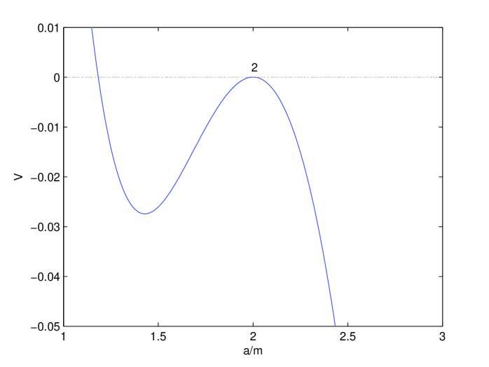
Figure 1: The wormhole is unstable.

down around $a_{0}/m=2$, showing that the wormhole is unstable.

As another example, if $a_{0}/m=3.5$ and $l/m=1.7$, we obtain $2(l/m)^{2}=5.78$, $2+4\omega=-0.6528$, and

$$V(a)=1-\frac{2(a/m)^{2}}{(a/m)^{3}+5.78}-\left[1-\frac{2(3.5)^{2}}{3.5^{3}+5.78}\right]\left(\frac{3.5}{a/m}\right)^{-0.6528}.$$ (24)

The graph, shown in Fig. 2, is concave up

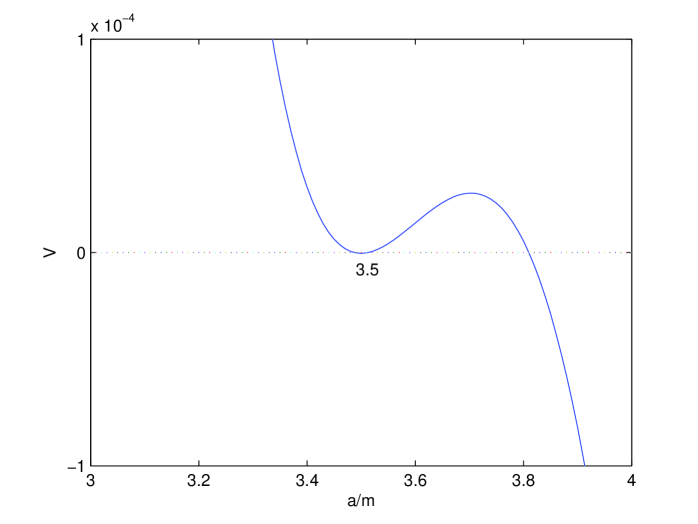
Figure 2: The wormhole is stable.

around $a_{0}/m=3.5$. So the wormhole is stable.

Table 1 provides an overview of the results for various values of $a_{0}/m$, starting with $a_{0}/m=1.5$ by showing the dependence on the Hayward parameter: to ensure stability, a larger value of $a_{0}/m$ requires a larger value of $l/m$. (For $a_{0}/m\leq 1$, we get only unstable solutions.)

$\boldsymbol{a_{0}/m}$	$\boldsymbol{l/m}$	Status
1.5	$\sqrt{16/27}$	unstable
1.5	0.8	stable
2	0.9	unstable
2	1.0	stable
2.5	1.1	unstable
2.5	1.2	stable
3	1.3	unstable
3	1.4	stable
3.5	1.6	unstable
3.5	1.7	stable
4	1.9	unstable
4	2.0	stable
4.5	2.2	unstable
4.5	2.3	stable
5	2.6	unstable
5	2.7	stable

Table 1: Larger values of $a_{0}/m$ require larger values of $l/m$ for stability.

Since we are dealing with compact objects rather than black holes, we need to check the physical plausibility. Consider a typical neutron star having a radius ranging from 11 km to 11.5 km and a mass of $2M_{\odot}\approx 3\,\text{km}$. Then $a_{0}/m$ ranges from 3.67 to 3.83, which are well within the values listed in Table 1. In fact, it is theoretically possible to have a stable thin shell right above the surface with $a_{0}/m=4$ and $l/m=2.0$ according to Table 1.

Other compact objects such as quark stars or strange stars could allow even smaller values for $a_{0}/m$.

6 Conclusion

This paper introduces a new type of thin-shell wormhole constructed from a special class of compact stellar objects rather than black holes. This finding follows from a discussion of the stability to linearized radial perturbations of an extended version of a regular Hayward black hole. Assuming the equation of state $\mathcal{P}=\omega\sigma$, $\omega<0$, for the exotic matter on the thin shell, it is shown that whenever the value of the Hayward parameter is below its critical value, no stable solutions can exist. Stable solutions are obtained, however, if $l/m$ is allowed to exceed the critical value, thereby eliminating the event horizon of the black hole. The resulting underlying structure supporting the thin-shell wormhole is a compact object rather than a black hole. The findings are consistent with the properties of neutron stars, as well as other compact stellar objects.

References

- [1] M. Visser, “Traversable wormholes from surgically modified Schwarzchild spacetimes,” Nucl. Phys. B 328, 203 (1989).
- [2] M.S. Morris and K.S. Thorne, “Wormholes in spacetime and their use for interstellar travel: A tool for teaching general relativity,” Amer. J. Phys. 56, 395 (1988).
- [3] E.F. Eiroa, “Thin-shell wormholes with a generalized Chaplygin gas,” Phys. Rev. D 80, 044033 (2009).
- [4] P.K.F. Kuhfittig, “The stability of thin-shell wormholes with a phantom-like equation of state,” Acta Phys. Polon. B 41, 2017 (2010).
- [5] E. Poisson and M. Visser, “Thin-shell wormholes: Linearized stability,” Phys. Rev. D 52, 7318 (1996).
- [6] F.S.N. Lobo and P. Crawford, “Linearized stability analysis of thin-shell wormholes with a cosmological constant,” Class. Quant. Grav. 21, 391 (2004).
- [7] E.F. Eiroa and G.E. Romero, “Linearized stability of charged thin-shell wormholes,” Gen. Rel. Grav. 36, 651 (2004).
- [8] M. Thibeault, C. Simeone, and E.F. Eiroa, “Thin-shell wormholes in Einstein-Maxwell theory with a Gauss-Bonnet term,” Gen. Rel. Grav. 38, 1593 (2006).
- [9] F. Rahaman, M. Kalam, and S. Chakraborty, “Thin shell wormholes in higher dimensional Einstein-Maxwell theory,” Gen. Rel. Grav. 38, 1687 (2006).
- [10] F. Rahaman, M. Kalam, and S. Chakraborty, “Gravitational lensing by a stable C-field wormhole,” Chin. J. Phys. 45, 518 (2007).
- [11] M.G. Richarte and C. Simeone, “Thin-shell wormholes supported by ordinary matter in Einstein-Gauss-Bonnet gravity,” Phys. Rev. D 76, 087502 (2007).
- [12] J.P.S. Lemos and F.S.N. Lobo, “Plane symmetric thin-shell wormholes: Solutions and stability,” Phys. Rev D 78, 044030 (2008).
- [13] S.A. Hayward, “Formation and evaporation of nonsingular black holes,” Phys. Rev. Lett. 96, 031103 (2006).
- [14] M. Halilsoy, A. Ovgun, and S. Habib Mazharimousavi, “Thin-shell wormholes from regular Hayward black hole,” Eur. Phys. J. C 74, 2796 (2014).
- [15] M. Sharif and S. Mumtaz, “Stabilty of regular Hayward thin-shell wormholes,” Ad. High Energy Phys. 2016, 2868750, (2016).
- [16] C.W. Misner, K.S. Thorne, and J.A. Wheeler, Gravitation. W. Freeman and Company, New York (1973) p. 608.