Output Range Analysis for Deep Neural Networks
Abstract
Deep neural networks (NN) are extensively used for machine learning tasks such as image classification, perception and control of autonomous systems. Increasingly, these deep NNs are also been deployed in high-assurance applications. Thus, there is a pressing need for developing techniques to verify neural networks to check whether certain user-expected properties are satisfied. In this paper, we study a specific verification problem of computing a guaranteed range for the output of a deep neural network given a set of inputs represented as a convex polyhedron. Range estimation is a key primitive for verifying deep NNs. We present an efficient range estimation algorithm that uses a combination of local search and linear programming problems to efficiently find the maximum and minimum values taken by the outputs of the NN over the given input set. In contrast to recently proposed “monolithic” optimization approaches, we use local gradient descent to repeatedly find and eliminate local minima of the function. The final global optimum is certified using a mixed integer programming instance. We implement our approach and compare it with Reluplex, a recently proposed solver for deep neural networks. We demonstrate the effectiveness of the proposed approach for verification of NNs used in automated control as well as those used in classification.
Introduction
Deep neural networks have emerged as a versatile and popular representation model for machine learning due to their ability to approximate complex functions and the efficiency of methods for learning these from large data sets. The black box nature of NN models and the absence of effective methods for their analysis has confined their use in systems with low integrity requirements but more recently, deep NNs are also been adopted in high-assurance systems such as automated control and perception pipeline of autonomous vehicles (?). While traditional system design approaches include rigorous system verification and analysis techniques to ensure the correctness of systems deployed in safety-critical applications (?), the inclusion of complex machine learning models in the form of deep NNs has created a new challenge to verify these models. In this paper, we focus on the range estimation problem, wherein, given a neural network and a polyhedron representing a set of inputs to the network, we wish to estimate a range for each of the network’s output that subsumes all possible outputs and is “tight” within a given tolerance . We restrict our attention to feedforward deep NNs. Furthermore, the NNs are assumed to use only rectified linear units (ReLUs) (?) as activation functions. Adapting to other activation functions will be discussed in an extended version.
Despite these restrictions, the range estimation problem has several applications. Consider a deep NN classification model with the last layer neural units, before the soft-max computation to determine the class label, denoted by . Given an image , denotes the value of the -th last layer neural unit for the input and denote a compact polyhedron region around modeling perturbations of the image . The range of label for the polyhedron input is denoted by . Label is possible for a perturbation of input in if and only if is not empty. Hence, we can verify if a label is possible for a given set of perturbations of image by solving the range estimation problem. This will establish the robustness of the deep NN classification models. Another application of the range estimation problem is to prove the safety of deep NN controllers by proving bounds on the outputs generated by these models. This is important because out of bounds outputs can drive the physical system into undesirable configurations such as the locking of robotic arm, or command a car’s throttle beyond its rated limits. Finding these errors through verification will enable design-time detection of potential failures instead of relying on runtime monitoring which can have significant overhead and also may not allow graceful recovery. Additionally, range analysis can be useful in proving the safety of the overall system.
Related Work
The importance of analytical certification methods for neural networks has been well-recognized in literature. (?) present one of the first categorization of verification goals for NNs used in safety-critical applications. The proposed approach here targets criteria G4 and G5 in (?) which aim at ensuring robustness of NNs to disturbances in inputs, and ensuring the output of NNs are not hazardous. The verification of neural networks is a hard problem, and even proving simple properties about them is known to be NP-complete (?). The nonlinearity and non-convexity of deep NNs make their analysis very difficult.
There has been few recent results reported for verifying neural networks. A methodology for the analysis of ReLU feed-forward networks is studied in (?). Their approach relies on Satisfiability Modulo Theory (SMT) solving (?), while we only use a combination of gradient-based local search and MILP solving (?). The linear programming used for comparison in Reluplex (?) performs significantly less efficiently according to the experiments reported in this paper. Note, however, that the scenarios used by Katz et al. are different from those studied here, and are not publicly available for comparison. A related goal of finding adversarial inputs for deep NNs has received a lot of attention, and can be viewed as a testing approach to NNs instead of verification method discussed in this paper. A linear programming based approach for finding adversarial inputs is presented in (?). A related approach for finding adversarial inputs using SMT solvers that relies on a layer-by-layer analysis is presented in (?). The use of SMT solvers for analysis of NNs has also been studied in (?). In contrast, our goal is to not just find adversarial or failing inputs that violate some property of the output but instead, we aim at establishing the guaranteed range of the output for a given polyhedral region of possible inputs. An abstraction-refinement based iterative approach for verification of NNs was proposed in (?). It relies on abstracting NNs as a Boolean combinations of linear arithmetic SMT constraints that is guaranteed to be conservative. Spurious counterexamples arising due to abstraction are used to refine the encoding. Note that our approach can fit well inside such an abstraction-refinement framework.
Contributions
We present a novel algorithm for propagating convex polyhedral inputs through a feedforward deep neural network with ReLU activation units to establish ranges s for the outputs of the network. We have implemented our approach in a tool called sherlock. We compare sherlock with a recently proposed deep NN verification engine - Reluplex (?). We demonstrate the application of sherlock to establish output range of deep NN controllers as well as to prove the robustness of deep NN image classification models. Our approach seems to scale consistently to randomly generated sparse networks with up to neurons and random dense networks with up to neurons. Furthermore, we demonstrate its applications on neural networks with as many as neurons.
Preliminaries
We present the preliminary notions including deep neural networks, polyhedra, and mixed integer linear programs.
Deep Neural Networks
We will study feed forward neural networks (NN) using so-called “ReLU” units throughout this paper with inputs and a single output. Let denote the inputs and be the output of the network. Structurally, a NN consists of hidden layers wherein we assume (for simplicity) that each layer has neurons. We use to denote the neuron of the layer for and .
A layer neural network with neurons in each hidden layer is described by a set of matrices:
wherein (a) are and matrices denoting the weights connecting the inputs to the first hidden layer, (b) for connect layer to layer and (c) connect the last layer to the output.
Definition 1.1 (ReLU Unit).
Each neuron in the network implements a nonlinear function linking its input value to the output value. In this paper, we consider ReLU units that implement the function .
We extend the definition of to apply component-wise to vectors as .
Taking to be the ReLU function, we describe the overall function defined by a given network .
Definition 1.2 (Function Computed by NN).
Given a neural network as described above, the function computed by the neural network is given by the composition wherein is the function computed by the hidden layer with denoting the function linking the inputs to the first layer and linking the last layer to the output.
For a fixed input , we say that a neuron is activated if the value input to it is nonnegative. This corresponds to the output of the ReLU unit being the same as the input. It is easily seen that the function computed by a NN is continuous and piecewise affine, and differentiable almost everywhere in . If it exists, we denote the gradient of this function . Computing the gradient can be performed efficiently (as described subsequently).
Mixed Integer Linear Programs
Throughout this paper, we will formulate linear optimization problems with integer variables. We briefly recall these optimization problems, their computational complexity and solution techniques used in practice.
Definition 1.3.
A mixed integer linear program (MILP) involves a set of real-valued variables and integer valued variables of the following form:
The problem is called a linear program (LP) if there are no integer variables . The special case wherein is called a binary MILP. Finally, the case without an explicit objective function is called a MILP feasibility problem. It is well known that MILPs are NP-hard problems: the best known algorithms, thus far, have exponential time complexity in the worst case. In contrast, LPs can be solved efficiently using interior point methods.
Problem Definition
Let be a neural network with inputs , a single output and weights . Let be the function defined by such a network.
Definition 1.4 (Range Estimation Problem).
The range estimation problem is defined as follows:
-
•
Inputs: Neural network , input constraints and a tolerance parameter .
-
•
Output: An interval such that . I.e, contains the range of over inputs . Furthermore, we require the interval to be tight:
We will assume that the input polyhedron is compact: i.e, it is closed and has a bounded volume.
Overall Approach
Without loss of generality, we will focus on estimating the upper bound . The case for the lower bound will be entirely analogous. First, we note that a single MILP can be used to directly compute , but can be quite expensive in practice. Therefore, our approach will combine a series of MILP feasibility problems alternating with local search steps.
Figure 2 shows a pictorial representation of the overall approach. The approach incrementally finds a series of approximations to the upper bound , culminating in the final bound .
-
1.
The first level is found by choosing a randomly sampled point .
-
2.
Next, we perform a series of local iteration steps resulting in samples that perform gradient ascent until these steps cannot obtain any further improvement. We take .
-
3.
A “global search” step is now performed to check if there is any point such that . This is obtained by solving a MILP feasibility problem.
-
4.
If the global search fails to find a solution, then we declare .
-
5.
Otherwise, we obtain a new witness point such that .
-
6.
We now go back to the local search step.
Algorithm 1 presents the pseudocode for the overall algorithm. The procedure starts by generating a sample from the interior of (line 2) using an interior-point LP solver. Next, we iterate between local search iterations (line 5) and global search (line 7). Each local search call provides a new point and that is deemed a local minimum of the search procedure. We increment the current estimate by , the given tolerance parameter (line 6) and ask the global solver to find a new point such that is at least as large as the current value of (line 7). If this succeeds, then we update the current values of (line 9). Otherwise, we conclude that the current value of is a valid upper bound within the tolerance .
We assume that the procedures LocalSearch and GlobalSearch satisfy the following properties:
-
•
(P1) Given a point , the LocalSearch procedure returns such that .
-
•
(P2) Given a neural network and the current estimate , the GlobalSearch procedure either declares feasible along with such that , or declares not feasible if no satisfies .
We recall the basic assumptions thus far: (a) is compact, (b) and (c) properties P1, P2 apply to the LocalSearch and GlobalSearch procedures. Let us denote the ideal upper bound by .
Theorem 1.1.
Algorithm 1 always terminates. Furthermore, the output satisfies .
Proof.
Since is compact and is a continuous function. Therefore, the maximum is always attained.
To see why it terminates, we note that the value of increases by at least each time we execute the loop body of the While loop in line 4. Furthermore, letting be the value of attained by the sample obtained in line 2, we can upper bound the number of steps by .
We note that the procedure terminates only if GlobalSearch returns infeasible. Therefore, appealing to property P2, we note that . Or in other words, .
Likewise, consider the value of returned by the call to LocalSearch in the last iteration of the loop, denoted as along with the point . We note that . Therefore, we have . However, . This completes the proof. ∎
Local and Global Search
In this section, we will describe the local and global search algorithms used in our approach for estimating upper bounds. The approach for estimating lower bounds is identical replacing ascent steps with descent steps.
Local Search Technique
The local search algorithm uses a steepest projected gradient ascent algorithm, starting from an input sample point and , iterating through a sequence of points , such that and .
The new iterate is obtained from as follows:
-
1.
Compute the gradient .
-
2.
Compute a “locally active region” .
-
3.
Solve a linear program (LP) to compute .
We now describe the calculation of , the definition of a “locally active region” and the setup of the LP.
Gradient Calculation:
Technically, the gradient of need not exist for each input . However, this happens for a set of points of measure , and is dealt with in practice by using a smoothed version of the function defining the ReLU units.
The computation of the gradient uses the chain rule to obtain the gradient as a product of matrices:
wherein represents the Jacobian matrix of partial derivatives of the output of the layer with respect to those of the layer . Since we can compute the gradient using the following simple rule:
-
1.
If the entry then copy row of to .
-
2.
Otherwise, set the row of to be all zeros.
In practice, the gradient calculation can be piggybacked onto the function evaluation so that we obtain both the output and the gradient .
First order optimization approaches present numerous rules such as the Armijo step sizing rules for calculating the step size (?). However, in our approach we exploit the local linear nature of the function around the current sample input to setup an LP.
Definition 1.5 (Locally Active Region).
For an input to the neural network , the locally active region describes the set of all inputs such that activates exactly the same neurons as .
Given the definition of a locally active region, we obtain the following property.
Lemma 1.1.
The region is described by a polyhedron with possibly strict inequality constraints. If , then .
Proof.
(Sketch). To see why is a polyhedron, we proceed by induction on the number of hidden layers at the network. Let be the subset of neurons in the first hidden layer that are activated by . We can write linear inequalities that ensure that for any other input , the inputs to the neurons in are and likewise the inputs to the neurons not activated in the first layer are . Proceeding layer by layer, we can write a series of constraints that describe . Since the gradient is entirely dictated by the set of active neurons, it is clear that . ∎
Let denote the closure of the local active set by converting the strict constraints to their non-strict versions. Therefore, the local maximum is simply obtained by solving the following LP.
The solution of the LP above yields a step of the local search.
Termination:
The local search is terminated when each step no longer provides a sufficient increase, or alternatively the length of each step is deemed too small. These are controlled by user specified thresholds in practice. Another termination criterion simply stops the local search when a preset maximum number of iterations is exceeded. In practical implementations, all three criteria are used.
We note that local search described thus far satisfies property P1 recalled below.
Lemma 1.2.
Given a point , the LocalSearch procedure returns a new , such that .
Global Search
We will now detail the global search procedure. The overall goal of the global search procedure is to search for a point such that for a given estimate of the current upper bound. The approach formulates a MILP feasibility problem, whose real-valued variables are:
-
1.
: the inputs to the network with variables.
-
2.
, the outputs of the hidden layer. Each is a vector of variables.
-
3.
: the overall output of the network.
Additionally, we introduce binary () variables , wherein each vector has the same size as . These variables will be used to model the piecewise behavior of the ReLU units.
Now we encode the constraints. The first set of constraints ensure that . Suppose is defined as then we simply add these as constraints.
We wish to add constraints so that for each hidden layer , holds. Since is not linear, we use the binary variables to encode the same behavior:
Note that for the first hidden layer, we simply substitute for . This trick of using binary variables to encode piecewise linear function is standard in optimization (?, Ch. 22.4) (?, Ch. 9). Here is taken to be a very large constant as a placeholder for . Additionally, we can derive fast estimates for by using the norms and the bounding box of the input polyhedron.
The output is constrained as: . Finally, we require that .
The MILP, obtained by combining these constraints, is a feasibility problem without any objective.
Lemma 1.3.
The MILP encoding is feasible if and only if there is an input such that .
Experimental Evaluation
We first describe our C++ implementation of the ideas described thus far, called sherlock. sherlock combines local search with the commercial MILP solver Gurobi, freely available for academic use (?). The tolerance parameter is fixed to .
For comparison with Reluplex, we used the proof of concept implementation available at (?). However, at its core, Reluplex does not compute intervals. Therefore, we use a bisection scheme to repeatedly query Reluplex with ever smaller intervals until, we have narrowed down the actual range within a tolerance .
| Network Params. | sherlock | Reluplex | ||||||||||||
| # Iters | ||||||||||||||
| avg | min | max | avg | min | max | avg | min | max | ||||||
| 2 | 2 | 10 | 0.5 | 100 | 0.47 | 0.0 | 1.95 | 3.5 | 2 | 17 | 66 | 2.5 | 1.0 | 2.6 |
| 3 | 2 | 10 | 0.5 | 100 | 0.72 | 0.0 | 4.6 | 4.8 | 2 | 15 | 71 | 4 | 0.85 | 11.0 |
| 4 | 5 | 10 | 0.5 | 100 | 4.6 | 0.01 | 25.2 | 4.8 | 2 | 19 | 53 | 207.5 | 21.8 | 1036.3 |
| 5 | 8 | 10 | 0.05 | 100 | 0.01 | 0 | 0.02 | 2 | 2 | 2 | 3 | 1.65 | 1.2 | 1.89 |
| 5 | 8 | 10 | 0.2 | 100 | 0.16 | 0.01 | 1.93 | 2 | 2 | 3 | 7 | 6.1 | 1.9 | 11 |
| 5 | 8 | 10 | 0.5 | 64 | 40 | 0.03 | 1023.4 | 4.5 | 2 | 31 | 12 (*8) | 621.6 | 121.7 | 1025.7 |
| 5 | 8 | 10 | 0.8 | 44 | 167 | 0.18 | 1068.8 | 3 | 2 | 11 | 0 | x | x | x |
| 5 | 8 | 10 | 0.95 | 40 | 51 | 0.2 | 1201 | 2.5 | 2 | 4 | 0 | x | x | x |
| 10 | 2 | 10 | 0.5 | 99 | 1.65 | 0.0 | 7.74 | 24 | 2 | 104 | 86 (*1) | 42.1 | 1.6 | 339.7 |
| 10 | 5 | 10 | 0.5 | 91 | 16.5 | 0.02 | 86.4 | 22 | 2 | 407 | 7 | 433.2 | 23.2 | 1111.2 |
| 10 | 5 | 50 | 0.05 | 99 | 6.7 | 0.08 | 76.5 | 3 | 2 | 12 | 32 (*1) | 70.3 | 9 | 452 |
| 10 | 5 | 50 | 0.2 | 8 | 354.8 | 0.2 | 1429.1 | 2 | 2 | 3 | 0 | x | x | x |
| 10 | 5 | 50 | 0.4 | 8 | 35.4 | 1.6 | 114.5 | 3 | 3 | 3 | 0 | x | x | x |
| 10 | 5 | 50 | 0.5 | 0 | x | x | x | x | x | x | 0 | x | x | x |
Randomly Generated Networks
First, we generate numerous randomly generated networks with output by varying the number of inputs (), the number of hidden layers (), the number of neurons per hidden layer () and the fraction of non-zero edge weights (). Columns 1-4 of Table 1 shows the set of values chosen for . For each chosen set, we generated random neural networks. The zero weight edges were chosen by flipping a coin with probability of choosing a weight to be zero. The nonzero weights were uniformly chosen in the range . Next, we compare our approach against Reluplex solver assuming that the inputs are in the range . Each tool is run with a timeout of minutes. Table 1 shows the comparison. sherlock outperforms Reluplex in terms of the number of examples completed within the given timeout. However, we note that many of the Reluplex instances failed before the timeout due to an “error” reported by the solver. From the table we conclude that the total number of neurons and the sparsity of the network have a large effect on the overall performance. In particular, no approach is able to handle dense examples with neurons.
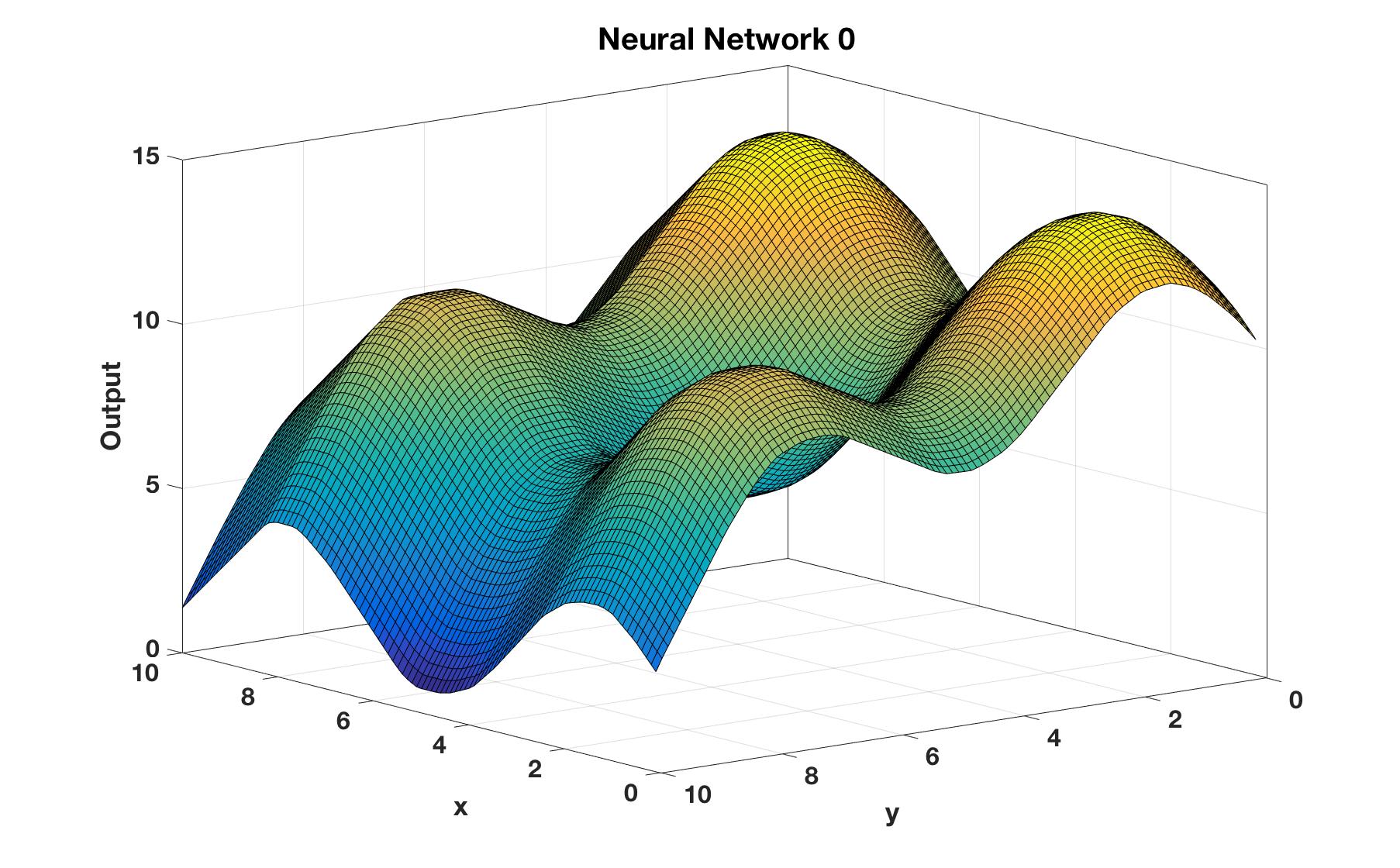
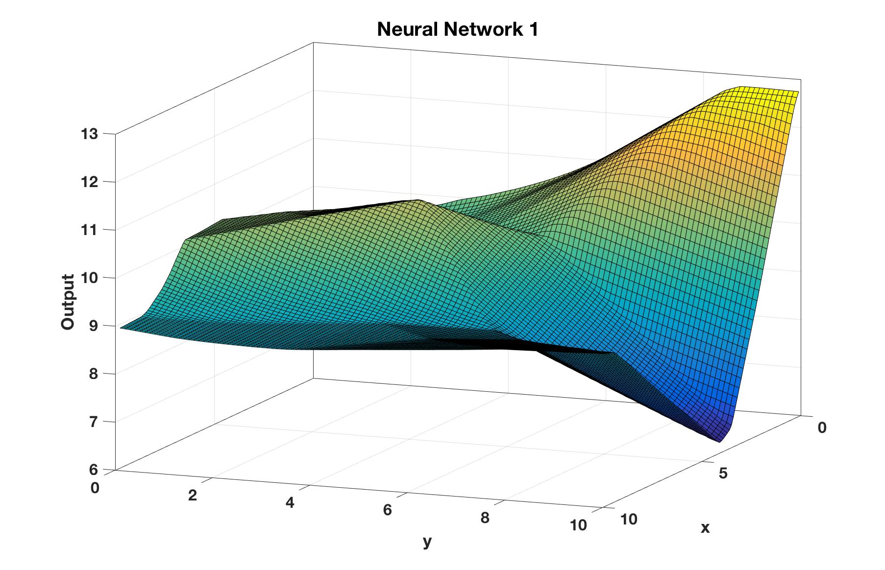
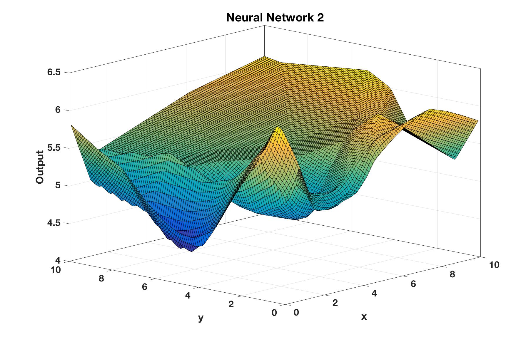
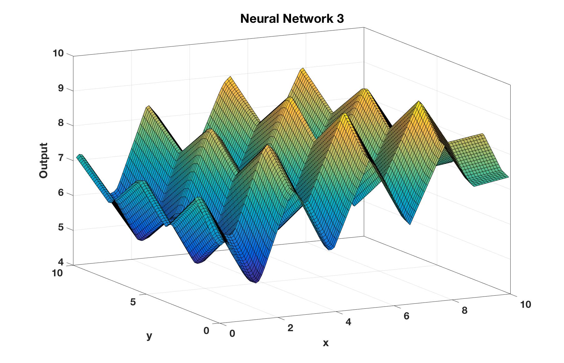
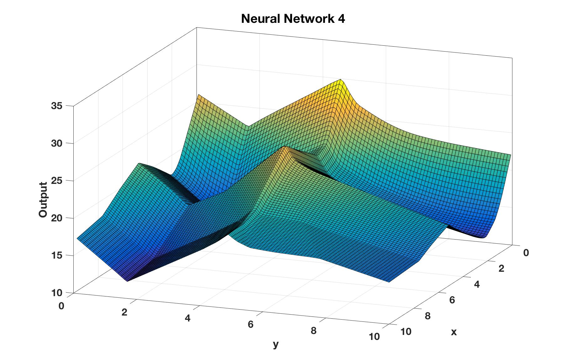
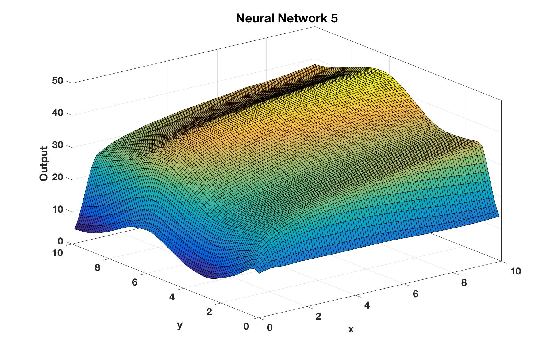
Microbenchmarks on Known Functions
Next, we consider a set of microbenchmarks that consist of networks trained on known input, single output functions shown in Figure 3. These functions provide varying numbers of local minima. We then sampled inputs/output pairs, and trained a neural network with hidden layer for the first functions and hidden layer for the last. Next, we compared sherlock against the Reluplex solver in terms of the ability to predict the output range of the function given the input range for the two inputs.
Table 2 summarizes the results of our comparison. We note that in all cases, our approach can solve the resulting problem within minutes. However, with a timeout of hour, Reluplex is unable to deduce a range for out of instances.
| ID | |||
|---|---|---|---|
| 1 100 | 1.9s | 1m 55s | |
| 1 200 | 2.4s | 13m 58s | |
| 1 500 | 17.8s | timeout | |
| 1 500 | 7.6s | timeout | |
| 1 1000 | 7m 57.8s | timeout | |
| 6 250 | 9m 48.4s | timeout |
Illustrative Applications
We illustrate the use of sherlock to infer properties of deep NNs for important applications, starting with a neural network that controls a nonlinear system. As mentioned earlier, such networks are increasingly popular using deep policy learning (?).
We trained a NN to control a nonlinear plant model (Example 7 from (?)) whose dynamics are describe by the ODE:
We first devise a model predictive control (MPC) scheme to stabilize this system to the origin, and train the NN by sampling inputs from the state space and using the MPC to provide the corresponding control.
We trained a 3 input, 1 output network, with 2 hidden layers, having 300 neurons in the first layer and 200 neurons in the second layer. For any state , we seek to know the range of the output of the network to deduce the maximum/minimum control input. This is a direct application of the range estimation problem. sherlock is able to deduce a tight range for the control input: .
Handwriting Recognition Networks
We illustrate an application of range estimation to large neural networks involved in pattern classification, wherein, we wish to infer classification labels for images. The MNIST handwriting recognition data set has emerged as a prototype application (?).
Given a neural network classifier , and a given image input , we wish to explore a set of possible perturbations to the image to find a nearby input that can alter the label that provides to the perturbed image. Alternatively, given a space of possible perturbations, we wish to prove that the network is robust to these perturbations: i.e, no perturbation can alter the label that provides to the perturbed image.
We trained a NN with inputs, and outputs, and hidden layers with and neurons in the layers respectively on the MNIST digit recognition data set (?). The network has outputs that are then fed to a “softmax” output layer to provide the final classification. For the purposes of our application, we remove this softmax layer and examine these outputs that represent numerical scores corresponding to the digits .
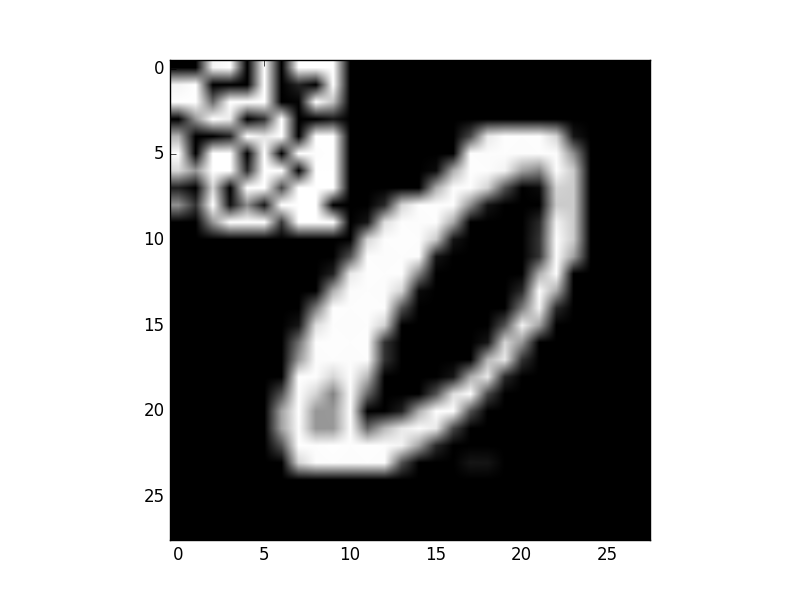
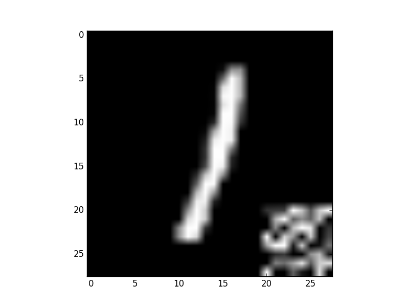
We first use our approach to generate adversarial perturbations to the images, which can flip the output. To do so, we define for each image a set of pixels and a range of possible perturbation of these pixels. This forms a polyhedron that we will call the perturbation space. Next, we use our approach to explore points in this perturbation space, stopping as soon as we obtain a point with a different label. This is achieved simply using local search iterations. Figure 4, demonstrates such an effect, we started with images that are classified correctly as the digits “0” and “1”. The perturbations are applied to selected pixels resulting in the digit “0” labeled as “8”, and “1” labeled as “2”.
However, rather finding a perturbation, we wish to prove robustness to a class of perturbations. I.e, for all possible perturbations, the label ascribed by the network to an image remains the same.
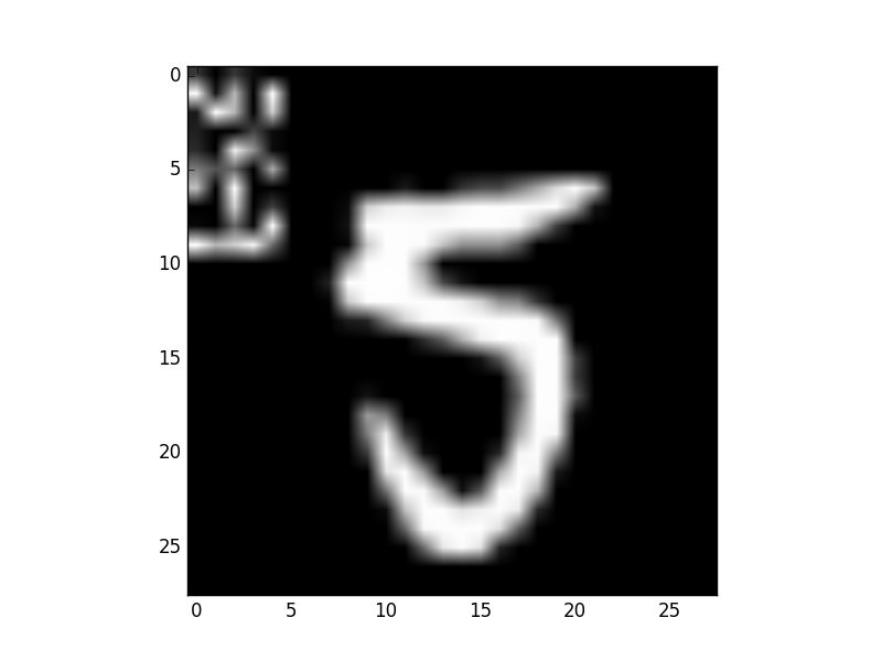
We chose an image labeled as and specified a set of perturbations to a block of size on the top left corner of the image. One such perturbation is shown in Figure 6. We used sherlock to compute a range over the output labels for all such perturbations. Figure 5 shows the output ranges for each label. It is clear that all perturbations will lead the softmax layer to choose the label over all other labels for the image.
Conclusion
Thus, we have presented a combination of local and global search for estimating the output ranges of neural networks given constraints on the input. Our approach has been implemented inside the tool sherlock and compared the results obtained with the solver Reluplex. We have also demonstrated the application of our approach to interesting applications to control and classification problems.
In the future, we wish to improve sherlock in many directions, including the treatment of recurrent neural networks, handling activation functions beyond ReLU units and providing faster alternatives to the MILP for global search.
References
- [Baier and Katoen 2008] Baier, C., and Katoen, J.-P. 2008. Principles of Model Checking. MIT Press.
- [Barrett et al. 2009] Barrett, C. W.; Sebastiani, R.; Seshia, S. A.; and Tinelli, C. 2009. Satisfiability modulo theories. Handbook of satisfiability 185:825–885.
- [Bastani et al. 2016] Bastani, O.; Ioannou, Y.; Lampropoulos, L.; Vytiniotis, D.; Nori, A.; and Criminisi, A. 2016. Measuring neural net robustness with constraints. In Advances in Neural Information Processing Systems, 2613–2621.
- [Bixby 2012] Bixby, R. E. 2012. A brief history of linear and mixed-integer programming computation. Documenta Mathematica 107–121.
- [Gurobi Optimization 2016] Gurobi Optimization, I. 2016. Gurobi optimizer reference manual.
- [Huang et al. 2016] Huang, X.; Kwiatkowska, M.; Wang, S.; and Wu, M. 2016. Safety verification of deep neural networks. CoRR abs/1610.06940.
- [Kahn et al. 2016] Kahn, G.; Zhang, T.; Levine, S.; and Abbeel, P. 2016. Plato: Policy learning using adaptive trajectory optimization. arXiv preprint arXiv:1603.00622.
- [Katz et al. 2017] Katz, G.; Barrett, C.; Dill, D. L.; Julian, K.; and Kochenderfer, M. J. 2017. Reluplex: An Efficient SMT Solver for Verifying Deep Neural Networks. Cham: Springer International Publishing. 97–117.
- [Katz et al. 2017] Katz et al. 2017. Reluplex: CAV 2017 prototype. https://github.com/guykatzz/ReluplexCav2017.
- [Kurd and Kelly 2003] Kurd, Z., and Kelly, T. 2003. Establishing safety criteria for artificial neural networks. In International Conference on Knowledge-Based and Intelligent Information and Engineering Systems, 163–169. Springer.
- [LeCun and Cortes 2010] LeCun, Y., and Cortes, C. 2010. MNIST handwritten digit database.
- [LeCun, Bengio, and Hinton 2015] LeCun, Y.; Bengio, Y.; and Hinton, G. 2015. Deep learning. Nature 521(7553):436–444.
- [Luenberger 1969] Luenberger, D. G. 1969. Optimization By Vector Space Methods. Wiley.
- [Pulina and Tacchella 2010] Pulina, L., and Tacchella, A. 2010. An abstraction-refinement approach to verification of artificial neural networks. In Computer Aided Verification, 243–257. Springer.
- [Pulina and Tacchella 2012] Pulina, L., and Tacchella, A. 2012. Challenging smt solvers to verify neural networks. AI Commun. 25(2):117–135.
- [Sassi, Bartocci, and Sankaranarayanan 2017] Sassi, M. A. B.; Bartocci, E.; and Sankaranarayanan, S. 2017. A linear programming-based iterative approach to stabilizing polynomial dynamics. In Proc. IFAC’17. Elsevier.
- [Vanderbei 2001] Vanderbei, R. J. 2001. Linear Programming: Foundations & Extensions (Second Edition). Springer. Cf. http://www.princeton.edu/~rvdb/LPbook/.
- [Williams 2013] Williams, H. P. 2013. Model Building in Mathematical Programming (Fifth Edition). Wiley.