Topology of large scale under-dense regions

Abstract

We investigate the large scale matter distribution adopting QSOs as matter tracer. The quasar catalogue based on the SDSS DR7 is used. The void finding algorithm is presented and statistical properties of void sizes and shapes are determined. Number of large voids in the quasar distribution is greater than the number of the same size voids found in the random distribution. The largest voids with diameters exceeding $300$ Mpc indicate an existence of comparable size areas of lower than the average matter density. No void-void space correlations have been detected, and no larger scale deviations from the uniform distribution are revealed. The average CMB temperature in the directions of the largest voids is lower than in the surrounding areas by $0.0046\pm 0.0028$ mK. This figure is compared to the amplitude of the expected temperature depletion caused by the Integrated Sachs-Wolfe effect.

1 Introduction

Statistical characteristics of matter distribution depend on a number of cosmological parameters. Albeit structures on various scales carry the information of cosmological relevance, matter agglomerations on the largest scales attract the greatest interest. This is simply because the large structures are rare, and partly because some ‘unusual’ accumulations of matter could impose unique constraints on the precision cosmology $\Lambda$CDM model. A question of identifying structures is of statistical nature and has a long history. It was recently discussed by Park et al. (2015). Here we examine statistics of large voids found in the SDSS DR7 quasar catalogue.

Space distributions of individual matter components – luminous matter, diffuse baryonic matter and dark matter – are strongly correlated, but not identical (e.g. Suto et al., 2004). Also individual types of galaxies do not follow one universal distribution pattern. It seems, however, that noticeable differences that show up at small scales, systematically disappear at large scales. In particular, it seems legitimate to assume that at scales of hundreds Mpc the distribution of baryonic matter follows that of the dark matter.

Quasars are suitable to study the matter distribution at the largest scales for several reasons. Being the most luminous active galactic nuclei, samples of quasars cover usually huge volumes. Magnitude limited samples of quasars show lower than normal galaxies radial density gradients because of strong cosmic evolution. This allows to construct voluminous data sets with low observational selection bias (e.g. Croom et al., 2001, see below). Clustering properties of quasars and galaxies are not distinctly different at small and medium scales (see Ross et al., 2009), what assures us that at scales of several hundreds Mpc quasar distribution is representative for the luminous matter distribution. To be more specific, the relationship between the spatial distribution of galaxies and quasars is expected to be linear, i.e. amplitudes of the relative fluctuations of both components are equal.

Numerous galaxy surveys reveal a variety of structures that span a very wide range of linear sizes. Early 3D maps show pronounced filaments and voids extending over $50$ and more Mpc (Tarenghi et al., 1979; Chincarini et al., 1983; Huchra et al., 1983; de Lapparent et al., 1986). Still larger structures based on the SDSS have been reported; in particular, the Sloan Great Wall $420$ Mpc long (Gott et al., 2005), and the largest filamentary structure extending above $1$ Gpc found in the DR7QSO catalogue (Clowes et al., 2013). However, statistical significance of the latter one was questioned by Park et al. (2015) on the grounds that group finding algorithm used by Clowes et al. (2013) was not sufficiently restrictive and structures formed by chance were recognized as physical quasar group.

A question of distinction between ‘real’ and ‘by chance’ structures is crucial for statistical studies of the largest matter accumulations observed in the Universe. Long filaments may arise as a result of a coherent process that involves simultaneously adequately big amount of matter, or may be a product of chance alignment of separate ‘short’ filaments (Park et al., 2015). Likewise, large volumes of low matter density may develop from a single large scale fluctuation, or be a close group of ‘normal’ voids similar to those observed in the local Universe. In the present paper we address this last question. Distribution of quasars in the SDSS DR7 catalogue is investigated in respect of the number and size of empty regions (voids). Then, shapes of voids and void correlation is examined.

All distances and linear dimensions are expressed in co-moving coordinates. To convert redshifts to the co-moving distances, we use the flat cosmological model with $H_{\rm o}=70$ km s^-1Mpc^-1, $\Omega_{\rm m}=0.30$ and $\Omega_{\Lambda}=0.70$. We focus our study on the area between $3000$ and $4500$ Mpc, what corresponds approx. to the redshift range $0.8-1.6$.

The present investigation seems to belong to a broad field of galaxy distribution studies that adopt a void concept. However, our work is rather weakly related to this area. This is because of several reason. The most conspicuous are the void scale and definition. Here we examine voids with radii above $145$ Mpc that are completely empty. i.e. with no objects inside. Such zero-one approach is usually dropped in the galaxy studies. In our geometrical attitude to void definition we ignore kinematic effects of deviations from the Hubble flow. The redshift – distance relationship is determined by the cosmological model. Also, questions on dynamics of the large scale inhomogeneities of the matter distribution cannot be addressed here at the present stage.

Concentration of quasars is several orders of magnitude lower than the galaxy space density. Consequently, the area nominally covered by the DR7 QSO catalogue is sparsely populated with the average distance between neighbouring quasars of $r_{\rm n}\sim 125$ Mpc. Statistical relationship between the galaxy and quasar space distribution holds for scales considerably larger than $r_{\rm n}$, and only voids covering several $r_{\rm n}$ indicate areas of the actually low galaxy density and the low total matter density. Because of that, our analysis of quasar voids properties is limited to the largest voids. An advanced method to investigate topology of continuous fields in cosmology, namely a watershed void finder (WVF), has been developed in recent years (Platen, van de Weygaert & Jones, 2007). WVF is a particularly effective tool to study evolution of complex, hierarchical structures both in the real data and simulations (van de Weygaert, 2016, and references therein). The observational material is practically always represented by the discrete samples, and transformation of the discrete distribution into the continuous one constitutes the inherent element of the WVF method (Schaap & van de Weygaert, 2000). Here we will examine scales only a few times larger than the average quasar separations (see below). Voids in the present situation are defined by just a few objects, what does not allow for a credible construction of the continuous density field.

N-body simulations show that in scales of few dozens MPC void properties evolve with time (Sheth & van de Weygaert, 2004). Because the present investigation concentrates on much larger structures than typical voids observed in galactic catalogues, and we concentrate on a single large volume contained within a relatively narrow range of redshifts ($0.8\lesssim z\lesssim 1.6$), no cosmic evolution effects are considered in the paper.

Voids detected in galaxy surveys span a wide range of sizes. For instance, Lares et al. (2017) identify voids in the SDSS DR7 galaxy catalogue with radii in the range $6-24\,h^{-1}$ Mpc. Only relatively small and moderate size voids are almost completely devoid of galaxies (van de Weygaert, 2016). Linear sizes of the present voids exceed $300$ Mpc, and are comparable to the largest voids detected in the galaxy distribution (Stavrev, 2000). Such large volumes are called voids because of distinctly lower than average number of galaxies. However, the amplitude of density fluctuation within large voids is not well determined (Kopylov & Kopylova, 2002). Most information on this question is obtained from N-body large scale simulations (Nadathur et al., 2017). Also the present investigation cannot provide direct information on the distribution of galaxies in the areas coinciding with the quasar voids. One of the objectives of our paper is to measure the amplitude of the Integrated Sachs-Wolfe signal generated by the largest voids. Potential correlation between the cosmic microwave background (CMB) temperature variations with the quasar voids would confirm the physical nature of voids, and – in the future – could be used to measure amplitude of the large scale density fluctuations.

The paper is organized as follows. In the next section we present geometric construction that is used to define voids. In Sec. 3 a short description of the quasar sample used in the investigation is given. Statistical characteristics of voids found in the data are presented in Sec. 4. Number of voids, their sizes and shapes are parametrized by a sphere radius used in the void finding algorithm. Correlation of the sky position of the largest voids with the CMB temperature local minima is discussed in Sec. 5. Some peculiarities in void shapes are discussed in Sec. 6. Main results are summarized in Sec. 7. Statistics of voids in a random point distribution and details of the computer algorithm applied to find voids are given in the Appendices.

2 The void – definition

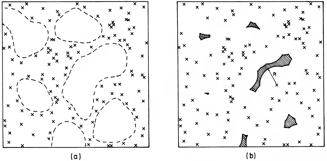
Figure 1: (a) Empty regions isolated by visual inspection and (b) shaded areas – void centres of voids size $R$ (from Soltan, 1985).

Large and roughly spherical areas devoid of galaxies together with galaxy clusters, walls and filaments constitute a complex structures of the galaxy distribution known as a cosmic web. Thus, the notion of cosmic voids was developed with the advent of the extensive galaxy surveys. The galaxy voids are easily identified visually in 3D surveys, but are also revealed in 2D massive counts such as the Lick galaxy counts.

Space concentration of quasars is much lower than that of galaxies. Thus, the apparent void in the quasar distribution does not imply presence of the comparable size galaxy void. Nonetheless, assuming no bias in the large scale distribution of quasars and galaxies, large quasar voids found in the present study indicate areas of the lower concentration of galaxies.

To analyze quantitatively even the basic void parameters, such as size and shape, one should replace the vague concept of void as a rounded empty volume by more rigorous void definition. Consequently, cosmic voids have been defined in diverse ways in the past. It has been established that most galaxy voids are not totally empty, and this observations were incorporated in various void investigations. In the present study the void is defined as a region completely devoid of objects. Figs. 1 (a) and (b), which are taken from Soltan (1985), illustrate in 2D a relationship between: (a) – the common realization of ’void’ notion, and (b) – the geometric construction representing the void. Let us consider the distribution of $n$ objects in the selected volume $V$. This distribution contains a void of size $R$ if one can insert into $V$ a circle (sphere in 3D) of radius $R$ with no objects inside. Shaded areas in Fig. 1 (b) indicate the underlying constructions of $n(R)=6$ voids of size $R$. It is convenient to call each of these areas a ’void centre’. Rigorously, the shaded areas are the geometric places of all the points which are centres for empty circles (spheres in 3D) of radius $R$.

One should note that shape of the void centre contains the information on the shape of the entire void. Both number of void centres and their shapes depend on the radius $R$, and – obviously – on the statistical characteristics of the distribution of points. Soltan (1985) gives the formula for the expected number of voids (void centres), $n(R)$, as a function of number of objects, $N$, volume, $V$, and $R$ for the Poissonian distribution of points in 2D and 3D (see also Appendix A).

3 The data

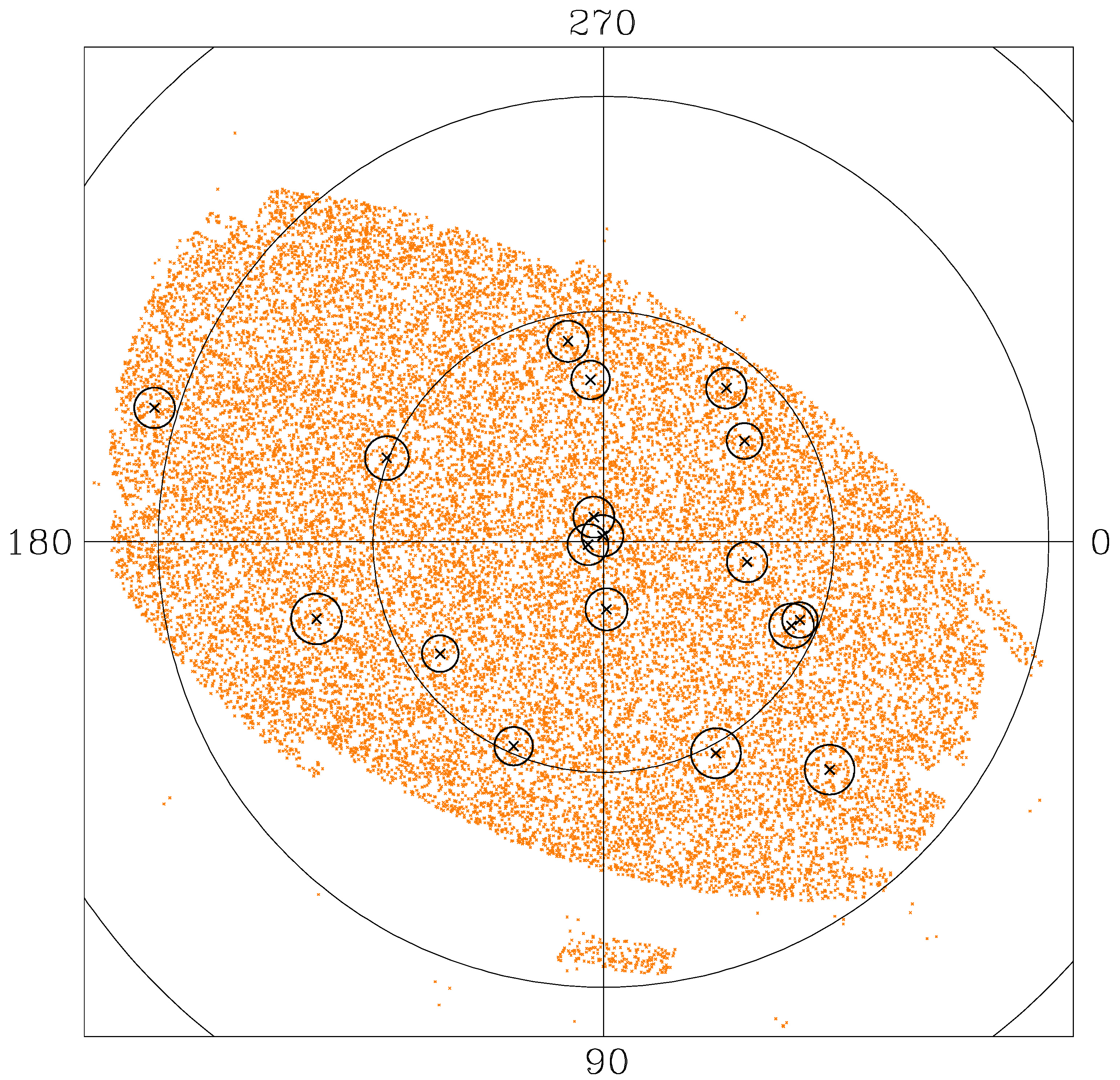
Figure 2: Distribution of $\sim 31000$ quasars from the SDSS DR7 quasar catalogue at distances between $2750$ and $4750$ Mpc in the north galactic hemisphere, brighter than $z=19.50$. Galactic latitude circles of $60^{\circ}$, $30^{\circ}$ and $0^{\circ}$ (arcs) are marked. A sample of voids with radii in the range of $177-193$ Mpc is shown; circles indicate the angular sizes of voids (see Sec. 5).

The Sloan Digital Sky Survey Quasar Catalogue is used to study potential inhomogeneities in the matter distribution on very large scales, i.e. above $\sim 300$ Mpc. The fifth edition of this catalogue is presented in Schneider et al. (2010). The multi step procedure to identify quasars, collect photometry and spectroscopic redshifts is described in that paper. Also the references to papers presenting all the successive releases of the catalogue are given. Total number of quasars in the catalogue exceeds $105\,000$, of which more than $90\,000$ lie in the northern galactic hemisphere. The redshifts range from $0.065$ to $5.46$, and $80$ per cent of them are between $0.55$ and $2.8$ ($2050$ Mpc and $6150$ Mpc).

Generally, the catalogue is magnitude limited what determines the overall distance distribution. Nevertheless, the distribution of objects in the redshift magnitude plane is complex what reflects multiple criteria applied to construct the final list of objects. In particular, quasar identification and redshift measurement depend on the position of emission lines in the SDSS photometric system and spectral band pass. Potentially this effect could introduce spurious variations of the redshift distribution for the catalogued objects. However the authors stated that this is not an issue for quasars in this catalogue. In the paper we investigate the quasar space distribution in the redshift range $\sim\!0.8~{}\div\sim\!1.6$. In this area the resultant selection (see Fig. 4 of Schneider et al. 2010) apparently generates flat space density distribution of the catalogued objects.

Void analysis, as other statistics dedicated to the space investigation, is hindered by the interference of the local effects with the cosmic data. Although large sections of the catalogue display a high degree of homogeneity, the surface distribution of objects in several regions of the celestial sphere is nonuniform and exhibits patches of distinctly different concentration of quasars. The observational material has been gathered for several years. Its homogeneity inevitably suffers from instrument-related biases as well as from the specifics of the data processing. In particular, selected areas are subject to different magnitude limits. In effect, most of the distinct features clearly visible in the surface distribution are not related to the cosmic signal. Our analysis is more sensitive to various selection effects (in most cases - unrecognized) that vary across the sky rather than to the radial bias that acts uniformly over the whole investigated area. Hence, in the present investigation we introduce an additional magnitude limit of $19.5$ in the $z$ band. Albeit, this $z$ cut-off decreases the number of quasars in the northern hemisphere from above $90000$ to $72067$, it effectively reduces conspicuous surface structures, apparently of the local origin. The $z$ band, with its average wavelength of $893$ nm, is used to select a possibly homogeneous sample because it is least affected by interstellar extinction. Fig. 2 shows the distribution of quasars in the north galactic hemisphere between $2750$ and $4750$ Mpc selected from the original SDSS catalogue brighter than $z=19.50$. Despite its featureless appearance, the subsequent analysis will show that the space distribution of objects is not random.

In Fig. 3 the space density of the selected quasar sample is shown as a function of distance. Overall decline of the density with increasing distance results from an apparent magnitude selection. A wide plateau between $3000$ and $4500$ Mpc comes from a kind of interplay between the observational selection and quasar cosmic evolution. This flat density distribution is helpful for studies of large structures, including voids. In the paper we concentrate on this section of the data. Apparent depression in the distance range $4000-4300$  Mpc (centered at redshift of $1.4$) is discussed below.

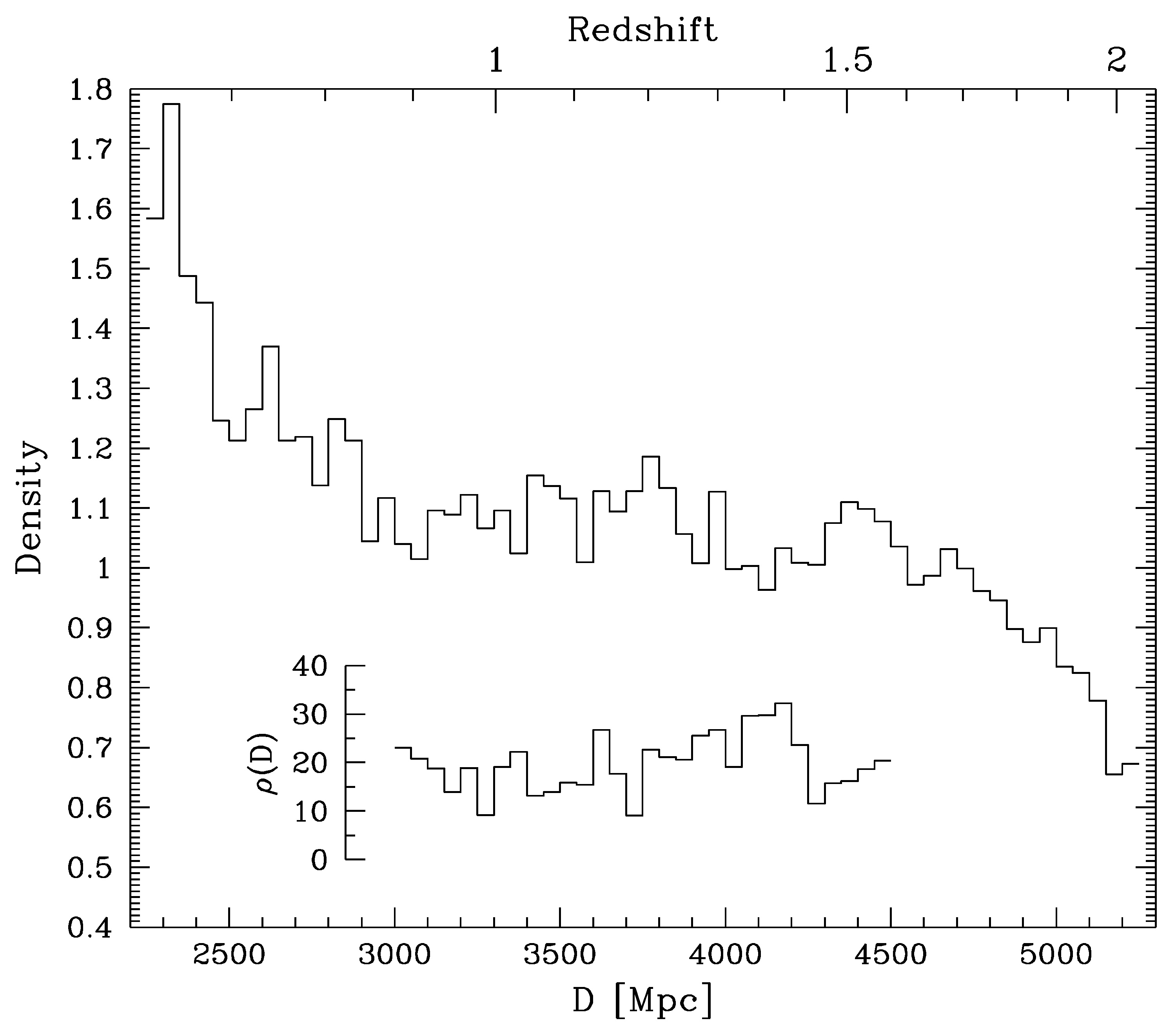
Figure 3: Radial distribution of quasars space density in the north galactic hemisphere (arbitrary units). The insert shows the density of the void centres in arbitrary units as a function of the distance (see Sec. 4).

4 Voids in the SDSS quasar distribution

Figure 4: Void centres projected onto celestial sphere for a selection of void sizes; numbers in the upper right corners give the void radii in Mpc.

The void centres in the northern galactic hemisphere were searched for at distances between $3000$ and $4500$ Mpc. All the calculations were performed with the resolution of $1$ Mpc in 3D. Te radial coordinates were determined from redshifts assuming the strict Hubble flow in the $\Lambda$CDM model. The computational details of the void finding algorithm are described in the Appendix B. The radius of the largest void in the investigated area $R=193$ Mpc. Fig. 4 shows the distributions of void centres projected on the sky for the selected void radii between $180$ and $145$ Mpc. The number of void centres, $n(R)$, grows as the radius decreases. Due to centre mergers the relationship is non-monotonic. However, within the radius range covered by the present computations, a rate at which ‘new’ centres emerge with decreasing radius, exceeds the rate of mergers. The effect of void mergers and the percolation phenomenon is illustrated in Appendix A where we show the analytic $n(R)$ relationship over a wide range of radii for the random distribution of points.

4.1 Space distribution of voids

The void centres occupy a small fraction of the investigated volume, $V=3.58\times 10^{10}$  Mpc³, over the entire range of void radii presented in Fig. 4. At the radius $R=145$ Mpc, the volume of all the void centres amounts to $1.96\times 10^{-3}$ of the $V$. The present radii are still distinctly greater than the percolation radius in the random (Poissonian) distribution of approximately $110$ Mpc. Thus, all the selected voids are situated at the ’large void’ tail of the void distribution. In this radius range, relatively small fluctuations of the space density of objects result in a strong variations of the void concentration (see Appendix A). Consequently, possible asymmetry of the void distribution on both sides of the galactic longitude line of $70^{\circ}-250^{\circ}$ (see bottom-right panel of Fig. 4), if real, may be a result of relatively small inhomogeneities of the survey rather than the true variations of the matter density on a Gpc scale.

Some insight into this question is provided by exploring the void distribution along the line of sight. The area between $3000$ and $4500$ Mpc is divided into approximately equal volumes. The near field extends between $3000$ and $3900$ Mpc, end the far one stretches from $3900$ to $4500$ Mpc. The distribution of void centres found for the radius of $145$ Mpc in both regions is shown in Fig. 5. The number of void centres in the more distant section is larger then in the near one by more then $26$ percent. The difference of void concentration in both fields has been expected because the quasar density in the more distant field shows a wide minimum centered at the distance of $\sim\!4100$ Mpc, or the redshift $z\approx 1.4$ (Fig. 3). Most likely this minimum is caused by the varying effectiveness of the line identification in quasar spectra (Schneider et al., 2010), and is unrelated to the intrinsic quasar distribution.

Figure 5: Void distribution at $R=145$ Mpc in two distance bins (in Mpc) indicated in the upper right corners.

It appears visually that void centre angular distributions in the celestial sphere in two distance bins exhibit overall similarities, what would indicate some inhomogeneities in the SDSS catalogue. However, it should be stressed that visually isolated differences of the distribution of void complexes, are not necessarily significant in the statistical terms. The whole population of void centres found at $R=145$ Mpc (Fig. 4, bottom right) does not show clear deviations from uniformity - the void centres are apparently scattered randomly. To investigate this question in a quantitative way, the observed distribution of separations between the void centres is analyzed. We compare the distribution of centre pairs in the real and random data sets.

According to the present definition, the void centre is a 3D object, often of a complex shape. Separation of two void centres is defined as a distance between their centres of mass. In the computations, the volume of the void centre is represented by a set of cubic cells $1$ Mpc a side (see Appendix B). Due to computer memory constraints, the void centre is identified and localized in space just by the cells distributed on the ‘centre surface’. Only these cells are kept for further analysis. Because of that, the position of the void centre is described by the centre of mass of the surface cells.

Two schemes to generate mock catalogues were applied. In the first one, angular positions of all the centres in the simulated data are the same as for the real ones, and randomized are only distances to the voids. We use the bootstrap method, and draw the random distances from the true distribution. In this case, the randomized void centres preserve some statistical characteristics of the real data. In the second method, a population of void centres found in strictly randomly distributed points is used.

We examine the distribution of centre pair separations for voids selected at radius $R=145$ Mpc. Let $p_{\rm d}(S)$ and $p_{\rm r}(S)$ denote the numbers of centre pairs with a separation $S$ normalized to the total number of pairs for the real and randomized void samples, respectively. A ratio of both quantities shifted to $0$ for the uncorrelated data represents a auto-correlation function (ACF) of void centres:

$$\xi(S)=\frac{p_{\rm d}(S)}{p_{\rm r}(S)}-1\,.$$ (1)

For both randomization schemes no correlation signal was detected. Fig. 6 shows results for the perfectly random data – within statistical fluctuations a ratio $p_{\rm d}(S)/p_{\rm r}(S)$ is equal to $1$. The pair separations in the random distribution are the average of $30$ data sets generated using the Monte Carlo scheme. The error bars represent the rms scatter between the simulations. No significant deviations of $p_{\rm d}(S)$ from the random case over a wide range of separations $S$ indicates that voids are not arranged into larger structures. Consequently, the distribution of voids provides no evidences for the under-dense areas significantly larger than the individual void.

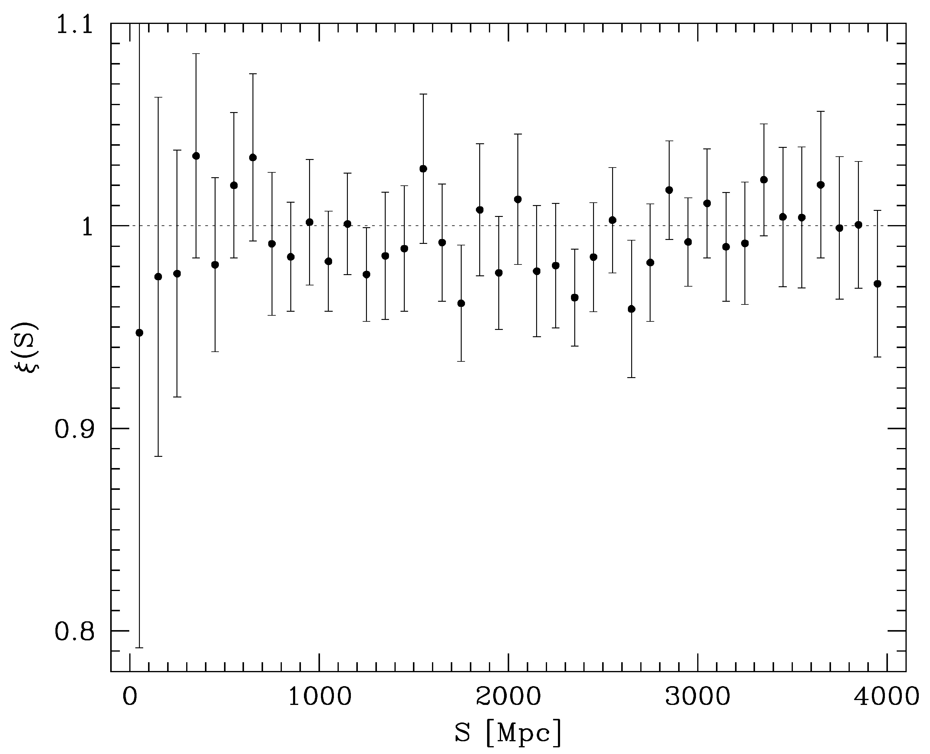
Figure 6: Auto-correlation function of void centres in 3D in $100$ Mpc bins. Error bars show a rms scatter between the mock random data.

4.2 Number of voids

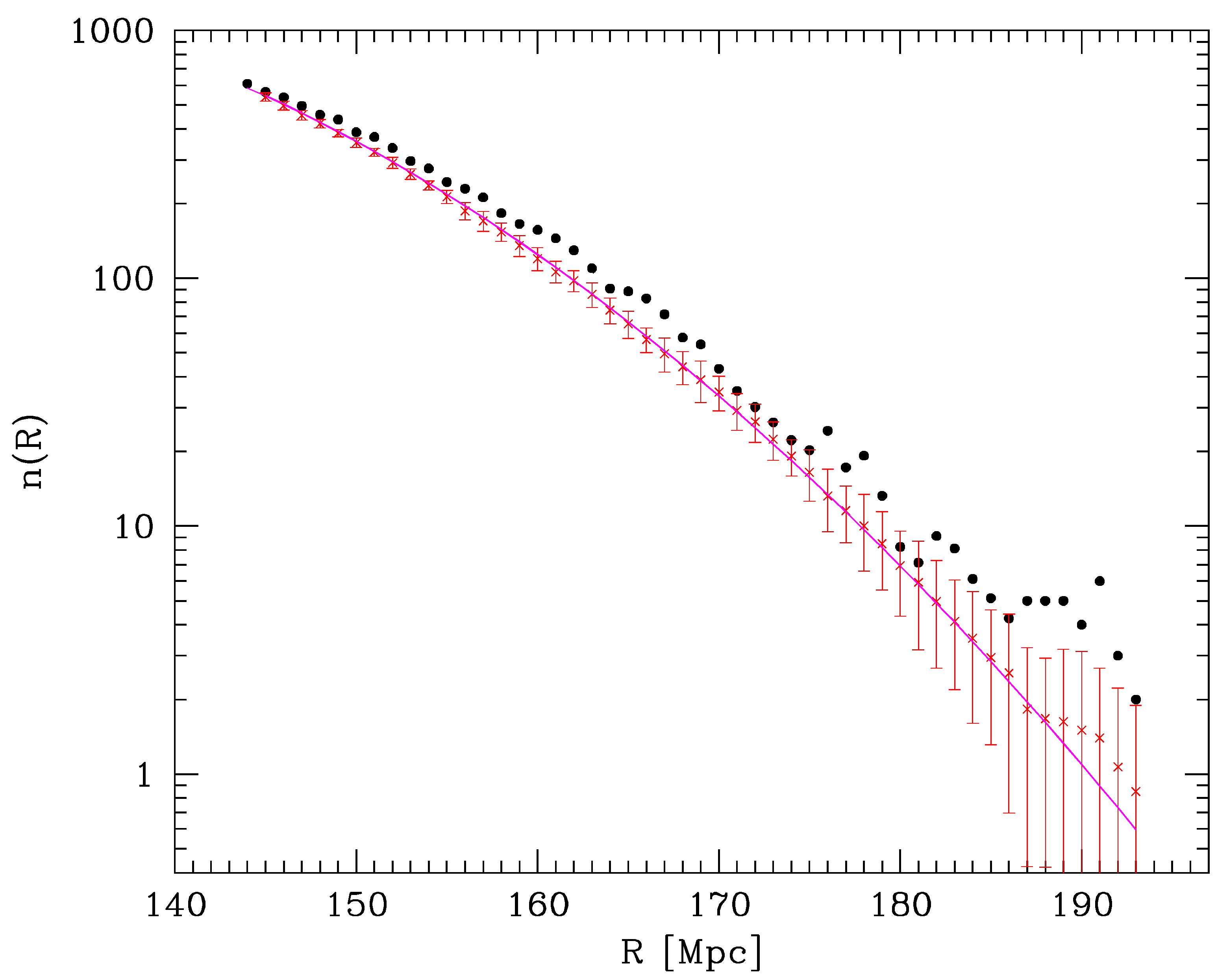
Figure 7: Number of void centres in the SDSS DR7 quasar catalogue: solid points are the real data; non-integer values indicate void centres reaching the edge of the search area; crosses with error bars – average of $30$ mock random distributions (see text for details).

Featureless surface distribution of quasars in the SDSS catalogue (Fig. 2) and close to uniform radial distribution (Fig. 3), indicate that any potential deviations from the the homogeneous space distribution of quasars are small at large scales. Therefore, the main objective of this analysis is to assess to what extent the true quasar distribution in fact differs from the random one. In the present analysis, the void statistics is used to determine the maximum linear scale at which the data exhibit non-random characteristics. To facilitate interpretation of the statistical void parameters, mock catalogues of uniformly distributed ’quasars’ have been constructed. Objects in the mock catalogues are randomly distributed in 3D using pseudo random number generator within a volume covered by the SDSS. Space density is equal to the average density in the true catalogue between $2750$ and $4750$ Mpc to allow for voids extending beyond the reference distance range of $3000-4500$ Mpc. A number of $30$ data sets were created to gain understanding on statistical scatter of the measured parameters.

The number of separate void centres in the true and simulated data as a function of radius is shown in Fig. 7. In order to account for the finite survey volume, the void centres are weighted according to their position relative to the area borders. The unit weight is given to all the centres that are completely contained in the analyzed volume. If the centre touches the boundary of the area at one face, the weight is reduce to $1/2$, if it touches two faces its weight is assumed to be equal to $1/4$, and for three faces - $1/8$. Thus, the total number of voids generally is not an integer. The error bars represent the rms dispersion determined for $30$ randomized catalogues. Over the whole range of void radii the real quasar data accommodate larger number of void centres, $n_{\rm d}(R)$, than the random simulated distributions, $n_{\rm r}(R)$. Although, the relative difference, $[n_{\rm d}(R)-n_{\rm r}(R)]/n_{\rm r}(R)$, fluctuates due to the stochastic nature of both distribution, the discrepancy between both quantities seems to decline steadily at the smaller radii. In the absolute numbers, the excess of true voids increases with diminishing radius, and stabilizes or begins to decrease below $r\approx 150$ Mpc.

The true void excess demonstrates that the void algorithm is an effective tool to investigate the large scale variations of quasar concentration and that the catalogued quasars are not distributed randomly in space. Apparently, the density of quasars is not perfectly constant in the investigated volume. Because of that, the number of large voids is greater than the number expected for the random distribution of objects populating the same volume with the density equal to the average density of quasars (see formula 5 for the number of voids in the Poissonian distribution).

It is likely that to some extent residual imperfections of the data selection procedures introduce some bias in the catalogue which is responsible for the the $n_{\rm d}(R)-n_{\rm r}(R)$ difference. To assess, how strongly the cosmic signal contributes to this difference, other statistical properties of voids are investigated in the following sections.

5 Voids vs. CMB

Fluctuations of matter distribution on very large scales influence the cosmic microwave background (CMB) what is known as the Integrated Sachs-Wolfe effect (ISW). CMB photons crossing mass agglomerations, as well as broad depressions of the mass density. gain or lose energy. Amplitude of the effect is defined by the net change of height of the potential hill (or depth of the well) during the photon travel time. In the matter dominated flat universe the time evolution of density fluctuations in the linear approximation is balanced by the matter dilution caused by the Hubble expansion and the effect is cancelled. In models with the cosmological constant the expansion of the universe is not matched by the evolution rate of density fluctuations and the ISW effect turns up.

From the observation point of view the ISW effect is still debatable. Although, the large structures (both superclusters and supervoids) found in extensive galaxy surveys, such as SDSS DR6 (Adelman-McCarthy et al., 2008), seem to correlate with the CMB temperature variations, the reported amplitude of the signal (e.g. Granett et al. 2008; Ilić et al. 2013; Kovács et al. 2017) is substantially larger than that expected for the ISW effect (e.g. Hernández-Monteagudo & Smith 2013; Hotchkiss et al. 2015).

Here, we explore the potential relationship between the voids found in the quasar catalogue and the CMB temperature fluctuations under the assumption that the correlation of both distributions is generated via the ISW effect. However, to confirm the existence of the under-dense regions associated with our voids, the nature of this correlation is not crucial. Obviously, if the observed void excess results from the catalogue deficiencies generated locally, one should expect no correlations of the detected voids with the CMB temperature. Moreover, the void excess can be generated by various kinds of fluctuations of the matter density that also do not introduce void - CMB correlation. For example, if the void excess is produced by variations of the density field on scales much larger than the present voids, the number of detected voids will exceed that for the Poissonian field, but a topology of individual voids will be defined just by geometrical structures unrelated to the local matter density. Only the physical connection of some voids with the true matter density depressions generates the sought correlation.

Figure 7 shows that the number of voids detected in the quasar distribution is greater than that expected in the perfect Poissonian case, but the relative difference of both quantities is rather modest. Thus, the majority of voids is not associated with the areas of lower than average matter density. Nevertheless, the systematic excess of the void number over a wide range of radii could indicate that some fraction of large voids is genetically related to the under-dense regions. We investigate in detail a possible coincidence of ‘cold spots’ in the CMB temperature map with the population of voids found in the present investigation. We note the obvious fact that the number of voids selected at two void radii are correlated. This is illustrated in Fig. 4, where all the voids selected at one radius show up also in the void maps constructed at all smaller radii. To obtain independent sets of void centres for different radii, we apply the following procedure. First, a void of the largest radius is found. It is centred at galactic coordinates $(l,b)=(216^{\circ},89^{\circ})$ at the distance of $4139$ Mpc. Then the centre of the next in size void is searched for, excluding the volume occupied by the first one. The minimum void centre separation equal to the radius of the larger void is introduced to eliminate the situation where several void centres are clustered in the small area. Such tight void group in fact represents potentially a single under-dense region. The second void with radius of $192$ Mpc is centred at $(l,b)=(309^{\circ},64^{\circ})$ at the distance of $4234$ Mpc. The procedure was repeated for all the voids down to $r=145$ Mpc, the smallest voids investigated here, and provided a list of $568$ void centres. A sky distribution of a sample of $18$ largest voids selected in this way in the radius range $193-176$ Mpc is shown in Fig. 2.

Figure 8: The CMB temperatures of all the voids grouped according to the void radius. The ordinate $\Delta T_{\rm CMB}$ shows the difference between the temperature in the direction of the void and the temperature in the annulus surrounding the void (see the text for details).

Figure 9: Distribution of void temperatures vs. distance and radius of voids with $R\geq 165$ Mpc.

The number of the observed voids with smaller radii approaches that predicted for the Poissonian case. These voids result from the purely random quasar structures and do not produce the ISW effect. Thus, the expected ISW signal averaged over the whole void population is highly diluted. Moreover, the fluctuations of the CMB temperature in the WMAP data at all the interesting scales are much larger than the expected ISW amplitude created by voids, what strongly reduces the signal-to-noise (S/N) ratio of the present ISW signal detection.

The CMB temperatures at direction of voids are calculated using the $9$ year WMAP CMB maps available at LAMBDA which is a part of NASA’s High Energy Astrophysics Science Archive Research Center. We used WMAP’s standard Res 9 HEALPix projection with $\sim 7$ arcmin resolution. For each void the CMB temperature was determined. The WMAP data were averaged over a circular sky area positioned at the void centre. One can expect that the highest amplitude of the ISW signal coincides with with the void centre and decays outside. To maximize the S/N ratio, the radius of the area was delineated as $\theta_{\rm CMB}=\varkappa\,\theta_{\rm void}$, with $\varkappa=0.9$, where $\theta_{\rm void}$ is the angular radius of a void (different values of $\varkappa$ give either the weaker signal or the stronger noise). The amplitude of the ISW signal was defined as the difference between the void temperature and the average CMB temperature in the surrounding area. The CMB map was smoothed using a spherical harmonic filter of degree $l=9$. The low value of the degree $l$ was chosen to produce sufficiently flat temperature map around each void. The reference temperature to calculate the ISW signal was assumed as the average temperature of the filtered CMB data in the annulus surrounding the void. The inner and outer annulus radii of $\theta_{\rm CMB}$ and $3\,\theta_{\rm CMB}$ were taken.

The $\Delta T_{\rm CMB}$ plotted in Fig. 8 show the differences between the void and reference temperatures in the set of $568$ voids defined above. The data are divided into $5$ bins according to the void radius:$145\leq R<148$ Mpc, $148\leq R<153$ Mpc, $153\leq R<159$ Mpc, $159\leq R<165$ Mpc, and $R\geq 165$ Mpc. The bins contain respectively: $125$, $155$, $136$, $69$, and $83$ voids. The cross shows the temperature difference for the merged two bins with largest radii ($R\geq 159$ Mpc). The $1\,\sigma$ uncertainties are estimated using the simulations. The void and reference temperatures were obtained for a set of $30$ randomized catalogues. The data have been processed in the same way as the original material, and the rms scatter of the corresponding $\Delta T_{\rm CMB}$ distributions in the mock catalogues is shown as the error bars. Details of the radial distribution and radii of voids with $R\geq 165$ Mpc are displayed in Fig. 9.

The distribution of temperatures in large voids is not symmetric with respect to the $\Delta T=0$ line. The average negative $\Delta T_{\rm CMB}$ signal for voids with $R\geq 159$ differs from zero by more than $1.64\,\sigma$, and in the highest bin of $R\geq 165$ Mpc the net temperature in $50$ voids is negative. Using the binomial distribution and assuming equal probabilities of temperatures below and above the average, a chance that at least $50$ of $83$ temperatures drawn at random will be negative amounts to $0.039$. In statistical terms, significance of this asymmetry is not very high. Nevertheless, the data are consistent with the correlation between the void distribution and the CMB temperature depressions, and it is legitimate to assume that some voids indeed coincide with the areas of lower than average matter density. Unfortunately, large intrinsic scatter of the CMB temperature maps strongly impedes assessing the amplitude of the ISW signal. This in turn, prevents us from imposing restrictive constraints on the density distribution in voids. Consequently, our objective in the subsequent calculations, is to examine to what extent the present estimates of $\Delta T_{\rm CMB}$ are consistent with the existing data on the large scale matter distribution derived from N-body simulations.

The relationship between the cosmic structures and the CMB temperature variations generated by the ISW effect has been broadly discussed in the past. In particular, a measurable correlation of the void distribution with depressions of the CMB temperature is expected in models with non-vanishing cosmological constant (e.g. Nadathur & Crittenden, 2016), although the predicted ISW signal is typically much weaker than those reported in the literature, (see Nadathur et al., 2014). Amplitude of $\Delta T$ depletion produced by the void depends on the time evolution of the gravitational potential, $\Phi(r)$, along the CMB photon path.

The distribution of $\Phi(r)$ in the vicinity of voids was investigated by Nadathur et al. (2017) using the N-body simulations. They found that for large voids, $\Phi(r)$ scales in a simple way with the void radius and the average galaxy density contrast within a void, $\delta_{g}=\rho_{\rm gv}/\rho_{\rm gl}-1$, where $\rho_{\rm gl}$ and $\rho_{\rm gv}$ are the global and void galaxy number densities, respectively. The approximate galaxy bias factor in voids is estimated at $2$. In the following we assume that these scaling relationships apply to the present voids, albeit the Nadathur et al. (2017) investigation concentrates on lower redshifts and smaller void sizes than those considered in the present paper. Thus, the subsequent calculations have only indicative character.

To assess capabilities to measure the large scale inhomogeneities of the matter distribution using the present void algorithm we apply the linear formula for the ISW temperature change (Nadathur & Crittenden, 2016):

$$\frac{\Delta T}{T}=-2\int_{0}^{z_{\rm LS}}a(z)[1-f(z)]\,\Phi\,dz\,,$$ (2)

where $z_{\rm LS}$ is the redshift of the last scattering, $a(z)$ – the cosmic scale factor, and

$$f=\frac{d\ln D}{d\ln a}\,,$$ (3)

is the density fluctuation growth rate, where $D(a)$ is the linear evolution of the matter density perturbation.

One can expect that the highest $\Delta T_{\rm CMB}$ amplitudes are generated preferentially by the largest voids. In the present investigation, however, the estimates of the average temperature signal are strongly affected by sampling errors. Because of that we include in the calculations all the voids with $R\geq 159$ Mpc. The average void radius in a sample of all the voids with $R\geq 159$ Mpc is $\overline{R}=167.7$ Mpc, and the average void distance $\overline{d}=3820$ Mpc ($\overline{z}\approx 1.2$). Using Nadathur et al. (2017) Eqs (6) and (10) with scaling coefficients in their Table B2, we get the distribution of potential, $\Phi(r)$, associated with the our ’average’ void for different amplitudes of the galaxy contrast $\delta_{g}$. Then, the integral in Eq. 2 is calculated in the $\Lambda$CDM cosmological model with parameters specified in the Introduction. The formulae for the linear growth rate, $D(a)$ were taken from Peebles (1980, p. 49–51).

To compare the model with our $\Delta T_{\rm CMB}$ estimates, we note that only a fraction of the voids is actually associated with the low density areas, while majority of voids results from random quasar configurations. Therefore, we define the average temperature signal produced by a true fluctuation of the matter distribution as:

$$\Delta T_{\rm u}=\eta\,\frac{\Delta T_{\rm v}\cdot n_{\rm v}}{n_{\rm v}-n_{\rm rv}}\,,$$ (4)

where $\Delta T_{\rm v}$ and $n_{\rm v}$ are the average temperature deficit in a void and the number of voids in the sample, and $n_{\rm rv}$ denotes the number of voids expected for the random distribution. The coefficient $\eta$ takes into account partial overlapping of voids, and is equal to the ratio of the total solid angle covered by voids to the summed up area of all the voids. For $R\geq 159$ and $\varkappa=0.9$ we have $\eta=0.753$, $\Delta T_{\rm v}=-0.00465\pm 0,0028$, and $n_{\rm v}=152$. The number of voids expected in the random distribution $n_{\rm rv}=126.9\pm 10.2$ is derived from $30$ mock catalogues. Thus, the temperature depletion associated with the under-dense regions $\Delta T_{\rm u}=-0.022\pm 0.016$ mK. According to Eq. 2 the temperature depletion at the level of $-0.022$ mK is produced by a void with the average density contrast of $\sim-0.62$. Although, the data on the galaxy distribution at redshifts under consideration are scarce, such high density contrasts seem unlikely. Also, the galaxy bias factor generally grows with redshift (e.g. Papageorgiou et al. 2012) and the corresponding galaxy concentration contrast would be even higher. Assuming large (as compared to the Nadathur et al. (2017) assessments) matter density contrast of $-0.3$, the temperature depletion according to Eqs 2 and 4 from our ‘average’ void $\Delta T_{\rm u}=-0.006$ mK, and $\Delta T_{\rm v}=0.0013$ mK. In view of the large CMB temperature variance, the ‘dilution’ of true underdense regions among the random quasar voids drastically reduces ability of the present method to investigate the ISW effect from voids.

We stress, that all these estimates are based on the extrapolation of the Nadathur et al. (2017) scaling relations for the relevant void parameters. Their distribution of void radii peaks at $\sim 40$ Mpc with no voids of $R$ above $90$ Mpc. Nadathur et al. (2012) assess that in $\Lambda$CDM models $\sim 100$ Mpc structures at $z\approx 0.5$ generate the ISW signal of $\lesssim 0.002$ mK. The hypothetical structures reported here exceed $300$ Mpc, and proportional higher temperature effect is expected. Such structures are, however, extremely rare. In the volume of $\sim 3.6\cdot 10^{10}$ Mpc, the number of under-dense regions associated with voids is estimated at $27\pm 10$. Thus, there is less than one such object in a cube of side $1100$ Mpc. It underlines the potential role of large void searches in the quasar distributions for the investigation of matter density fluctuations at scales much larger than accessible in the galaxy catalogues.

6 Void shapes

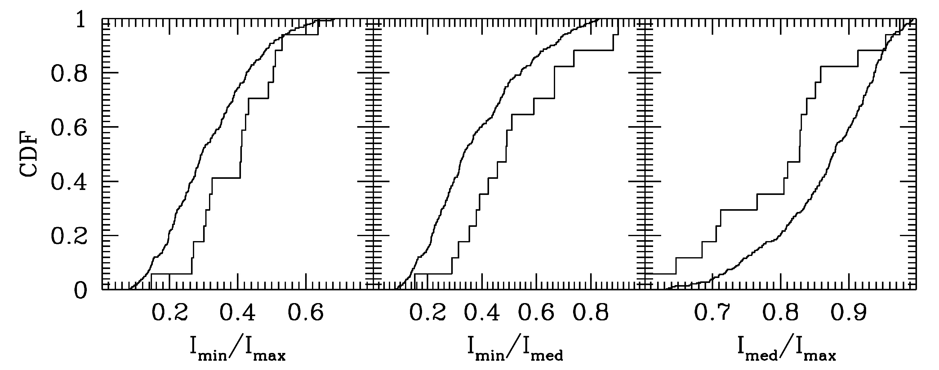
Figure 10: Cumulative distribution functions (CDF) of ratios of the principal moments of inertia: minimum to maximum, $I_{\rm min}/I_{\rm max}$, minimum to medium. $I_{\rm min}/I_{\rm med}$, and medium to maximum, $I_{\rm med}/I_{\rm min}$ for $17$ largest voids in the real data and for $242$ voids in $30$ sets of the randomized data. The voids were selected at the void radius $R=145$ Mpc.

A shape of the void centre is defined by cells distributed in the centre surface, as described in the Sec. 4.1. Obviously, shapes evolve with the void radius $R$. One can expect that statistical investigation of void centre structures should give also some insight into the typical properties of voids understood as volumes of space free of quasars. A moment of inertia is a natural tool to study the basic geometric properties of 3D structures. For that purpose, the void centre is considered as a rigid body.

Since the void centre is here represented only by cells in the outer layer of the spatially extended centre structure, the moment of inertia pertains just the ‘mass distribution’ of the surface of the centre. Principal moments of inertia and principal axes (eigenvalues and eigenvectors of the moment of inertia tensor) of void centres were calculated for the real and randomized data. Gross features of the centres, such as sizes, ratios of the principal moments, and directions of principal axes in both data sets were investigated. No conspicuous distinctions between the sets have been found, albeit some marginally significant differences in the centres shapes are present.

The distribution of quasars is a Poissonian stochastic process, and voids in the real data not necessarily reflect statistically significant large scale depression of the matter distribution. One can expect that preferably only the largest voids that are found occasionally in the real catalogue indicate areas of lower matter density. Among voids selected at $R=145$ Mpc, $17$ have ‘surface’ (as defined above) containing more that $1.5\cdot 10^{5}$ cubic $1$ Mpc cells. In the $30$ sets of the randomized distributions, only $242$ such large voids have been found. Fig. 10 shows the cumulative distribution functions, CDF, of the principal moments of inertia ratios for the real data ($17$ step functions) and the randomized data.

A two sample K-S test applied to the distributions of the principal moments of inertia, $I_{\rm max}$, $I_{\rm med}$, $I_{\rm min}$, reveals possible differences of void centre shapes in the data and in the simulations. In Fig 10 the cumulative distribution functions (CDF) of $I_{\rm min}/I_{\rm max}$, $I_{\rm min}/I_{\rm med}$, and $I_{\rm med}/I_{\rm max}$ for the true and random voids are shown. The distributions differ at a significance level of $0.039$, $0.032$ and $0.006$, respectively. Relationships between three principal moments are also visualized in Fig. 11, where the distribution of $I_{\rm min}/I_{\rm max}$ vs. $I_{\rm min}/I_{\rm med}$ is shown for the void centres in the quasar data and in the mock catalogues. To compare both distributions we apply two-dimensional version of the K-S test developed by Peacock (1983). The test indicates that real and random data differ at significance level of $0.0073$. The signal in the Peacock’s test is produced by the apparent excess of void centres in the top-left quadrant of Fig. 11. Judging from this feature, it implies that the shapes of centres are generally less elongated (or more spherical) as compared to the random case. One should keep in mind, however, that the actual shapes of void centres of the large voids are highly different from the ‘regular’ shapes of triaxial ellipsoids.

Figure 11: Distribution of principal moments of inertia ratios for void centres containing more that $1.5\cdot 10^{5}$ cells (see text for explanation) in the real data (full dots) and in $30$ randomized catalogues (crosses).

7 Concluding remarks

We study the space distribution of quasars in the SDSS to assess the matter distribution on very large scales. A suitable quasar void finding algorithm allowed for the investigation of void sizes and shapes. An existence of structures involving groups of voids were also examined. The SDSS quasar catalogue, taken as a whole, is subject to various selection biases. A section of the catalogue that covers the redshift range of roughly $0.8-1.6$ was used in the paper. Although, this area seems the best fitted for this kind of investigation, the data also suffered from imperfections, what limited the present study. Potential inhomogeneities of the SDSS could affected overall space distribution of voids. Because of that we concentrate on void characteristics that are fairly immune to the survey deficiencies.

It is shown that the distribution of void sizes is inconsistent with the random distribution of quasars. The excess of the number of voids is observed for diameters above $\sim\!300$ Mpc. We examine the largest voids, since they most likely coincide with the underlying large scale low matter density (baryonic and dark) areas. To relate the present voids with the true depressions of the matter density, we investigate the angular correlation between the voids and the CMB temperature distribution. Such correlation is expected due to the ISW effect. It is found that the average temperature in the direction of large voids is lower then in the surrounding areas by a few $\mu$K in rough agreement with the ISW mechanism in the $\Lambda$CDM model. However, the statistical significance of the detection is too low to perform a quantitative analysis of the ISW effect. Excess of voids with the negative temperature deviation over those with the positive one among $152$ voids with $R\geq 159$ Mpc is significant at $0.039$ level. We conclude that the low significance of both statistics results from the fact that extraneous variations of the CMB temperature are much larger that the measured amplitude of the ISW signal.

The space autocorrelation function of void centres is determined. The ACF amplitude is consistent with no correlation signal over a whole accessible range of void separations. However, this conclusion is not highly restrictive due to large uncertainties of the ACF estimate. To improve the voids statistics, data covering wider redshift range would be required.

In statistical terms, the shapes of the quasar void centres define space structures of under-dense areas. Thus, investigation of quasar voids could provide valuable information on the large scale matter distribution. The observed void centre shapes and those found in the random distributions are statistically different, although the differences are not high. Shapes here are defined solely by the ratios of principal moments of inertia $I_{\rm min}/I_{\rm max}$ and $I_{\rm med}/I_{\rm max}$. Assuming that distributions of these parameters describe a population of triaxial ellipsoids, real objects tend to be more spherical as compared to the simulated ones. However, the true shapes of the largest void centres in Fig. 4 (bottom right panel) strongly differ from ellipsoids, and conclusions based on such approximation should be treated cautiously. We plan to extend the investigation of voids using quasars in other redshift ranges. Broader observational basis should help to clarify also this point of the present paper.

Appendix A Voids in Poissonian distribution

In Appendices we use terms ‘void’ and ‘void centre’ as defined in Sec. 2.

Although the space distribution of quasars listed in the SDSS catalogue is different from the random (Poissonian) one, it is instructive to compare the void centres characteristics of the real data with this idealized case. Additionally, analytic formula for the number of voids in the Poissonian case derived in Soltan (1985) allows us to check quality of the void finder computer algorithm.

A number of random mock catalogues in the SDSS area were generated using the Monte Carlo scheme. Then, the void centres were found applying the same method as for the real data (see below). Results averaged over $30$ mock catalogues are shown in Fig. 12 with dots. The error bars represent the rms dispersion of $30$ data sets around the average number of centres $n(R)$, divided by the square root of the number of sets. The volume searched for void centres, $V$, and the space density of points, $\lambda$ were chosen to match corresponding quantities in the the real catalogue. In our case $V=3.58\cdot 10^{10}$ Mpc³, and $\lambda=5.15\cdot 10^{-7}$ Mpc^-3. The total number of points within $V$, $N=V\lambda\approx 18400$. To account for the edge effects the mock catalogues were generated over the larger area stretching out $250$ Mpc around $V$.

The solid curve gives the expected number of centres according to the analytic formula (Soltan, 1985):

$$n(R)=V\lambda\,e^{-\frac{4}{3}\pi\,R^{3}\lambda}\,\left(\frac{\pi^{4}R^{6}\lambda^{2}}{6}-4\,\pi\,R^{3}\,\lambda+1\right)\,,$$ (5)

for parameters $V$ and $\lambda$ given above. Equation 5 was derived under the assumption that for given $R$, the void centres are not considerably larger than the sphere of radius $R$. Thus, the formula breaks down at radii just a couple percent greater than the percolation radius, $R_{\rm p}$, i.e. the radius at which the individual void centres merge and create an infinite web. In the present case $R_{\rm p}\approx 110$ Mpc.

Even small variations of the local average matter density have a substantial impact on space concentration of voids in the relevant range of radii. To illustrate a steep dependence of the void probability on the quasar density in the limit of large voids, we use the Eq. 5. The dotted curve in Fig. 12 shows the expected number of voids in the same volume for $10$ percent lower density, i.e. for $\lambda=4.64\cdot 10^{-7}$ Mpc^-3. At radius $R\approx 171$ Mpc the number of voids as compared to the original $\lambda$ is higher by a factor of $2$ and the ratio increases at greater $R$.

Figure 12: Number of voids for the random distribution of points in a volume $V=3.58\cdot 10^{10}$ Mpc³ with the concentration $\lambda=5.15\cdot 10^{-7}$ Mpc^-3: solid curve – the expected number according to formula 5, points with the error bars – computed number using the present algorithm from the mock data generated by the Monte Carlo method; the insert shows the data for $145\leq R\leq 155$ Mpc in greater details; dotted curve – the expected number of voids for the number density $10$ percent lower, i.e. $\lambda=4.64\cdot 10^{-7}$ Mpc^-3.

Appendix B Voids – numerical algorithm

Spatial resolution of all the computations is set to $1$ Mpc. To search the whole volume of $\sim\!3.6\cdot 10^{10}$ Mpc for the void centres, a several step procedure is applied. First, the volume is divided into $\sim\!8.7\cdot 10^{6}$ cubic ‘domains’ of $a=16$ Mpc a side. For given void radius $R$, a distance $d$ between the domain centre and each quasar is examined. If $d<R-a\sqrt{3}/2$, the domain is eliminated from further computations. Number of accepted domains, $n_{\rm ad}(R)$, rises rapidly with the decreasing $R$. So, for $R$ equal to $193$, $190$, $155$, and $145$ Mpc the corresponding numbers of domains are: $1$, $35$, $13544$, and $45720$. Then, space distribution of accepted domains is inspected, and domains are segregated into clusters, where a cluster is defined as a group of mutually contiguous domains. Each cluster hosts one or more void centres.

In the next step, each accepted domain is divided into $16^{3}$ $1$ Mpc ‘cells’. For the each cell the distance from the cell centre to the nearest quasar is determined. If it is smaller than $R$, the cell is removed. Obviously, the total number of saved cells raises with the decreasing $R$ proportionally to $n_{\rm ad}(R)$, and quickly becomes unmanageable. To facilitate computations over the entire interesting range of $R$, only the cells distributed on the surface of the void centre are saved for further processing. A removal of the ‘interior’ cells allows for the effective analysis of void structures, although, the numbers of kept cells are still quite big. The largest void found at radius $R=145$ Mpc contains more that $400\,000$ ‘surface cells’. Space arrangement of cells determines the distribution and shape of void centres. Cells are split into clumps of ‘neighbours’. An isolated clump of cells defines a single void centre. Two cells are assumed to be neighbours if their separation in each coordinate does not exceed $2$ Mpc. This particular separation was chosen to balance a discrete character of cell selection, despite the fact that the void centre is a continuous body.

Very good agreement between the number of voids detected in simulations and given by the Eq. 12 assures us that the present void finding algorithm not only generates correct void numbers, but delivers accurate information on all the remaining void characteristics, as shape details, mutual relationships and orientation relative to the coordinate system.

References

- Adelman-McCarthy et al. (2008) Adelman-McCarthy J. K., Agüeros M. A., Allam S. S., Allende Prieto C., Anderson K. S. J., Anderson S. F., Annis J., Bahcall N. A., Bailer-Jones C. A. L., Zucker D. B., 2008, ApJS, 175, 297
- Chincarini et al. (1983) Chincarini G. L., Giovanelli R., Haynes M. P., 1983, A&A, 121, 5
- Clowes et al. (2013) Clowes R. G., Harris K. A., Raghunathan S., Campusano L. E., Söchting I. K., Graham M. J., 2013, MNRAS, 429, 2910
- Croom et al. (2001) Croom S. M., Smith R. J., Boyle B. J., Shanks T., Loaring N. S., Miller L., Lewis I. J., 2001, MNRAS, 322, L29
- de Lapparent et al. (1986) de Lapparent V., Geller M. J., Huchra J. P., 1986, ApJ, 302, L1
- Gott et al. (2005) Gott III J. R., Jurić M., Schlegel D., Hoyle F., Vogeley M., Tegmark M., Bahcall N., Brinkmann J., 2005, ApJ, 624, 463
- Granett et al. (2008) Granett B. R., Neyrinck M. C., Szapudi I., 2008, ApJ, 683, L99
- Hernández-Monteagudo & Smith (2013) Hernández-Monteagudo C., Smith R. E., 2013, MNRAS, 435, 1094
- Hotchkiss et al. (2015) Hotchkiss S., Nadathur S., Gottlöber S., Iliev I. T., Knebe A., Watson W. A., Yepes G., 2015, MNRAS, 446, 1321
- Huchra et al. (1983) Huchra J., Davis M., Latham D., Tonry J., 1983, ApJS, 52, 89
- Ilić et al. (2013) Ilić S., Langer M., Douspis M., 2013, A&A, 556, A51
- Kopylov & Kopylova (2002) Kopylov A. I., Kopylova F. G., 2002, A&A, 382, 389
- Kovács et al. (2017) Kovács A., Sánchez C., García-Bellido J., Nadathur S., Crittenden R., Gruen D., Huterer D., Bacon D., Clampitt J., DeRose J., Dodelson S., Thomas D., Walker A. R., DES Collaboration 2017, MNRAS, 465, 4166
- Lares et al. (2017) Lares M., Ruiz A. N., Luparello H. E., Ceccarelli L., Garcia Lambas D., Paz D. J., 2017, ArXiv e-prints
- Nadathur & Crittenden (2016) Nadathur S., Crittenden R., 2016, ApJ, 830, L19
- Nadathur et al. (2017) Nadathur S., Hotchkiss S., Crittenden R., 2017, MNRAS, 467, 4067
- Nadathur et al. (2012) Nadathur S., Hotchkiss S., Sarkar S., 2012, J. Cosmology Astropart. Phys., 6, 042
- Nadathur et al. (2014) Nadathur S., Lavinto M., Hotchkiss S., Räsänen S., 2014, Phys. Rev. D, 90, 103510
- Papageorgiou et al. (2012) Papageorgiou A., Plionis M., Basilakos S., Ragone-Figueroa C., 2012, MNRAS, 422, 106
- Park et al. (2015) Park C., Song H., Einasto M., Lietzen H., Heinamaki P., 2015, Journal of Korean Astronomical Society, 48, 75
- Peacock (1983) Peacock J. A., 1983, MNRAS, 202, 615
- Peebles (1980) Peebles P. J. E., 1980, The Large-Scale Structure of the Universe. Princeton University Press, Princeton, New Jersey
- Platen et al. (2007) Platen E., van de Weygaert R., Jones B. J. T., 2007, MNRAS, 380, 551
- Ross et al. (2009) Ross N. P., Shen Y., Strauss M. A., Vanden Berk D. E., Connolly A. J., Richards G. T., Schneider D. P., Weinberg D. H., Hall P. B., Bahcall N. A., Brunner R. J., 2009, ApJ, 697, 1634
- Schaap & van de Weygaert (2000) Schaap W. E., van de Weygaert R., 2000, A&A, 363, L29
- Schneider et al. (2010) Schneider D. P., Richards G. T., Hall P. B., Strauss M. A., Anderson S. F., Boroson T. A., Ross N. P., Shen Y., 2010, AJ, 139, 2360
- Sheth & van de Weygaert (2004) Sheth R. K., van de Weygaert R., 2004, MNRAS, 350, 517
- Soltan (1985) Soltan A., 1985, MNRAS, 216, 537
- Stavrev (2000) Stavrev K. Y., 2000, A&AS, 144, 323
- Suto et al. (2004) Suto Y., Yoshikawa K., Dolag K., Sasaki S., Yamasaki N. Y., Ohashi T., Mitsuda K., Tawara Y., Fujimoto R., Furusho T., Furuzawa A., Ishida M., Ishisaki Y., Takei Y., 2004, Journal of Korean Astronomical Society, 37, 387
- Tarenghi et al. (1979) Tarenghi M., Tifft W. G., Chincarini G., Rood H. J., Thompson L. A., 1979, ApJ, 234, 793
- van de Weygaert (2016) van de Weygaert R., 2016, in van de Weygaert R., Shandarin S., Saar E., Einasto J., eds, The Zeldovich Universe: Genesis and Growth of the Cosmic Web Vol. 308 of IAU Symposium, Voids and the Cosmic Web: cosmic depression & spatial complexity. pp 493–523