Parsec Scale Faraday-Rotation Structure Across the Jets of 9 Active Galactic Nuclei

Abstract

A number of groups have recently been active in searching for gradients in the observed Faraday rotation measure (RM) across jets of Active Galactic Nuclei (AGNs) on various scales and estimating their reliability. Such RM structures provide direct evidence for the presence of an azimuthal magnetic field component, which may be associated with a helical jet magnetic field, as is expected based on the results of many theoretical studies. We present new parsec-scale RM maps of 4 AGNs here, and analyze their transverse RM structures together with those for 5 previously published RM maps. All these jets display transverse RM gradients with significances of at least $3\sigma$. This is part of an ongoing effort to establish how common transverse RM gradients that may be associated with helical or toroidal magnetic fields are in AGNs on parsec scales.

1 Introduction

The relativistic jets of Active Galactic Nuclei (AGNs) emit radio synchrotron emission, which can be linearly polarized up to about 75% in optically thin regions with uniform magnetic fields, with the polarization angle $\chi$ orthogonal to the projection of the magnetic field B onto the plane of the sky (Pacholczyk 1970). The degree of linear polarization is considerably lower in optically thick regions, up to 10–15%, with $\chi$ parallel to the projected B (Pacholczyk 1970).

In the standard theoretical picture of AGN jets offered by Blandford & Königl (1979), emission is observed only near and beyond the location in the jet outflow where the optical depth is near unity, $\tau\approx 1$, representing the transition between optically thick regions closer to the central engine and optically thin regions farther along the jet. This $\tau\approx 1$ surface is a theoretical construction that is located somewhere within the “core” observed in Very Long Baseline Interferometry (VLBI) images. Although there is a tendency to think broadly in terms of an optically thick core and optically thin jet, there is abundant evidence that the VLBI cores observed at centimeter wavelengths are in fact mixed regions of partially optically thick emission corresponding to the vicinity of the theoretical $\tau\approx 1$ surface and optically thin emission from the inner jet (see, e.g., Gabuzda 2015).

Table 1: Source properties
Source	Alternate	Redshift	pc/mas	Integrated RM	Original RM
	Name			(rad m-2)	Map Ref
0212+735	S5 0212+73	2.37	8.28	$+22\pm 1$	2
0300+470	4C +47.08	—	—	$+22\pm 6$	*
0305+039	3C 78	0.029	0.57	$+10\pm 2$	3
0415+379	3C 111	0.049	0.95	$-24\pm 11$	1
0945+408	4C +40.24	1.249	8.50	$+3\pm 1$	*
1502+106	OR 103	1.838	8.53	$+1\pm 2$	*
1611+343	DA406	1.4	8.50	$+15\pm 1$	2
2005+403	TXS 2005+403	1.736	8.55	$-171\pm 12$	2
2200+420	BL Lac	0.069	1.29	$-199\pm 1$	*
1 = Zavala & Taylor (2002); 2 = Zavala & Taylor (2003); 3 = Kharb et al. 2009;
* = This RM map not previously published

Table 2: Map properties
Source	Epoch	Figure	Freq	Beam	Peak	Lowest contour	BMaj	BMin	BPA
			(GHz)	Shape	(Jy/beam)	(%)	(mas)	(mas)	(deg)
0212+735	June 27, 2000	4	8.1	E	2.32	0.50	1.50	1.03	$-7.4$
0212+735	June 27, 2000	4	8.1	C	2.39	0.50	1.24	1.24	–
0300+470	Sept. 26, 2007	1	4.6	E	0.60	0.25	3.41	1.86	$-7.9$
0300+470	Sept. 26, 2007	1	4.6	C	0.60	0.25	2.50	2.50	–
0305+039	Sept. 10, 2005	3	5.0	E	0.34	0.25	3.30	1.38	$-8.1$
0305+039	Sept. 10, 2005	3	5.0	C	0.37	0.25	2.06	2.06	–
0415+379	June 27, 2000	4	8.1	E	0.83	0.25	1.99	0.98	$-2.8$
0415+379	June 27, 2000	4	8.1	C	0.92	0.25	1.40	1.40	–
0945+408	Sept. 26, 2007	1	4.6	E	0.78	0.50	3.98	2.07	$-9.5$
0945+408	Sept. 26, 2007	1	4.6	C	0.85	0.50	2.87	2.87	–
1502+106	Sept. 26, 2007	1	4.6	E	0.98	0.25	5.30	1.95	$-18.0$
1502+106	Sept. 26, 2007	1	4.6	C	1.03	0.25	3.20	3.20	–
1611+343	June 27, 2000	4	8.1	E	2.70	0.50	2.00	0.97	$-5.0$
1611+343	June 27, 2000	4	8.1	C	2.66	0.50	1.40	1.40	–
2005+403	June 27, 2000	4	8.1	E	1.02	1.00	2.31	1.47	$-14.0$
2005+403	June 27, 2000	4	8.1	C	1.12	1.00	1.84	1.84	–
2200+420	Sept. 26, 2007	2	4.6	E	1.75	0.50	3.97	1.69	$-23.7$
2200+420	Sept. 26, 2007	2	4.6	C	1.75	0.50	2.59	2.59	–
2200+420	Sept. 26, 2007	2	4.6	E	1.54	1.00	2.27	1.15	$-24.3$
2200+420	Sept. 26, 2007	2	4.6	C	1.56	1.00	1.60	1.60	–

Multi-frequency VLBI polarization observations provide information about the wavelength dependence of the parsec-scale polarization, in particular, Faraday rotation occurring at various locations between the emitting region and observer. When Faraday rotation occurs in regions of thermal (non-relativistic or only mildly relativistic) plasma outside the emitting region the rotation is given by

$$\chi_{obs}-\chi_{o}=\frac{e^{3}\lambda^{2}}{8\pi^{2}\epsilon_{o}m^{2}c^{3}}\int n_{e}{\mathbf{B}}\cdot d{\mathbf{l}}\equiv RM\lambda^{2}$$ (1)

where $\chi_{obs}$ and $\chi_{o}$ are the observed and intrinsic polarization angles, respectively, $-e$ and $m$ are the charge and mass of the particles giving rise to the Faraday rotation, usually taken to be electrons, $c$ is the speed of light, $\epsilon_{o}$ the permittivity constant, $n_{e}$ the density of the Faraday-rotating electrons, $\mathbf{B}$ the magnetic field, $d\mathbf{l}$ an element along the line of sight, $\lambda$ the observing wavelength, and RM (the coefficient of $\lambda^{2}$) is the Rotation Measure (e.g., Burn 1966). The action of external Faraday rotation can be identified using simultaneous multifrequency observations, through the linear $\lambda^{2}$ dependence, allowing the determination of both the RM (which reflects the electron density and line-of-sight B field in the region of Faraday rotation) and $\chi_{o}$ (the intrinsic direction of the source’s linear polarization, and hence the synchrotron B field, projected onto the plane of the sky).

Many theoretical studies and simulations of the relativistic jets of AGNs have predicted the development of a helical jet B field, which comes about due to the combination of the rotation of the central black hole and its accretion disk and the jet outflow (e.g. Nakamura, Uchida & Hirose 2001, Lovelace et al. 2002; see Tchekhovskoy and Bromberg 2016 for a recent example). Researchers have long been aware that the presence of a helical jet B field could give rise to a regular gradient in the observed RM across the jet, due to the systematic change in the line-of-sight component of the helical field (Perley et al. 1984, Blandford 1993). Statistically significant transverse RM gradients across the parsec-scale jets of more than 25 AGN have been reported in the refereed literature (e.g. Gabuzda et al. 2015 and references therein), interpreted as reflecting the systematic change in the line-of-sight component of a toroidal or helical jet B field across the jets.

The Monte Carlo simulations of Hovatta et al. (2012), Mahmud et al. (2013) and Murphy & Gabuzda (2013) clearly indicate that the key factors in determining the trustworthiness of an RM gradient (i.e., the probability that it is not spurious) are (i) monotonicity, (ii) the range of values encompassed by the gradient relative to the uncertainties in the RM measurements and (iii) steadiness of the change in the RM values across the jet (ensuring a seeming “gradient” is not due only to values in a few edge pixels), rather than the width spanned by the gradient. The second criterion reflects the result of the Monte Carlo simulations that, when an RM gradient encompasses values differing by at least $3\sigma$ and spans even a small distance comparable to one beamwidth, the probability that it is spurious is very low – less than 1%.

Mahmud et al. (2013), Gabuzda et al. (2014a, 2014b) and Motter and Gabuzda (2017) have carried out new Faraday-rotation analyses employing the empirical error formula of Hovatta et al. (2012), focusing on monotonicity, steadiness of the gradient across the jet and a significance of at least $3\sigma$ as the key criteria for reliability of observed transverse RM gradients. Results published earlier by Gabuzda et al. (2004, 2008) were reanalyzed using this same approach by Gabuzda et al. (2015), who also reported 8 new cases of monotonic, statistically significant transverse RM gradients across AGN jets based on previously published and unpublished maps.

In the current study, we have applied this approach to analyze 4 RM images previously published by Zavala & Taylor (2002, 2003), based on VLBA data at 7 frequencies between 8.1 and 15.2 GHz, 1 RM image published by Kharb et al. (2009) based on 3 frequencies between 5.0 and 15.3 GHz and 4 RM images published here for the first time, based on VLBA data at 6 frequencies between 4.6 and 15.4 GHz. All of these AGNs display statistically significant transverse RM gradients across their jets. This is part of a larger study aiming to build up statistics for AGN jets displaying transverse RM gradients with the ultimate goal of analyzing the collected properties of the RM gradients detected.

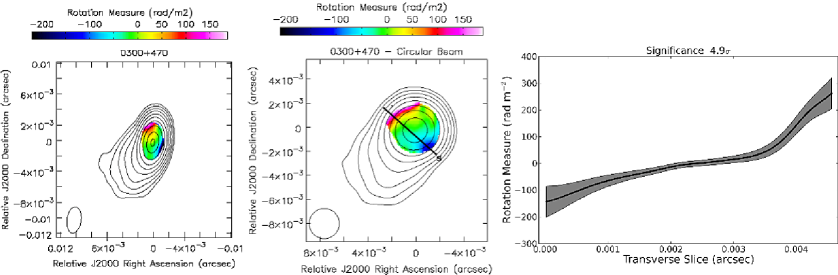
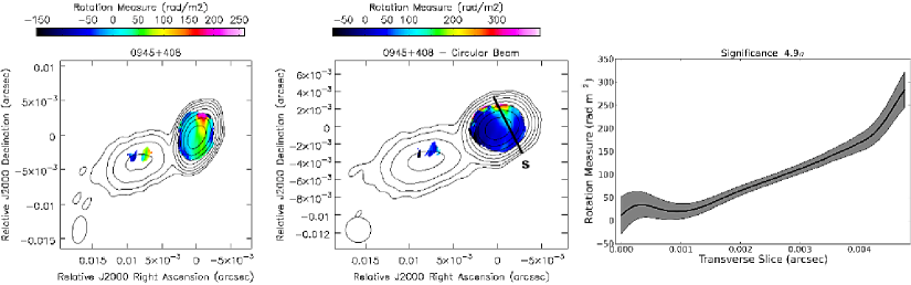
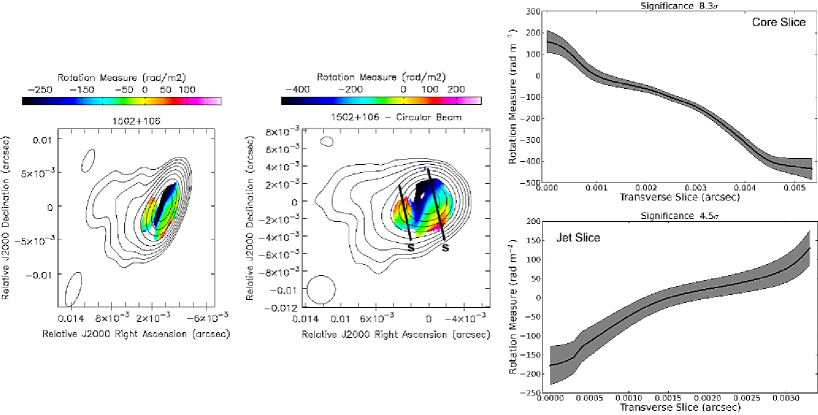
Figure 1: 4.6-GHz intensity maps and transverse Faraday RM gradients across the jets of 0300+470 (top), 0945+408 (middle) and 1502+106 (bottom), based on the 4.6–15.4 GHz data described in Section 2.1.

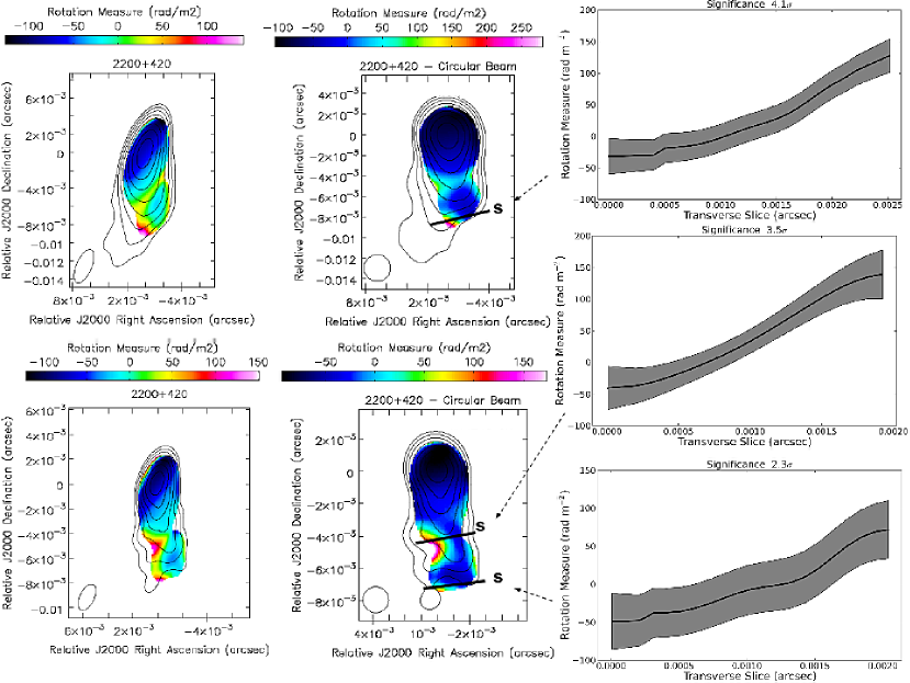
Figure 2: Transverse Faraday RM gradient across the jet of 2200+420, based on the 4.6–15.4 GHz data described in Section 2.1. The upper row of maps was made using the 4.6 GHz beam, while the lower row of maps correspond to the same data convolved with the (slightly smaller) 7.9-GHz beam.

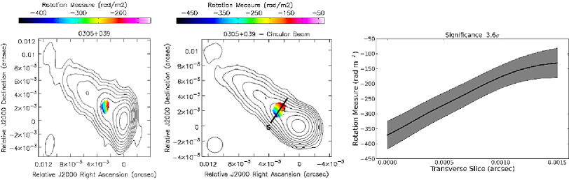
Figure 3: 5.0-GHz intensity maps and and transverse Faraday RM gradient across the jet of 0305+039, based on the 5.0–15.3 GHz data described in Section 2.2.

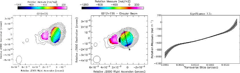
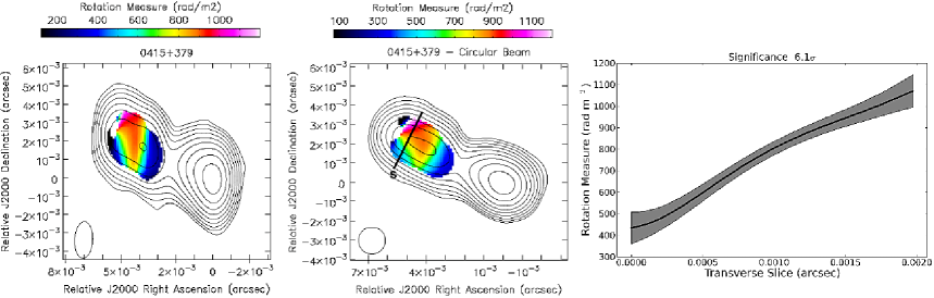
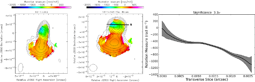
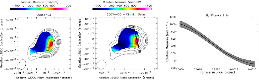
Figure 4: 8.1 GHz intensity maps and transverse Faraday RM gradients across the jets of 0212+735, 0415+379, 1611+343 and 2005+403, from top to bottom, based on the 8.1–15.2 GHz data described in Section 2.3.

2 Observations

Like Gabuzda et al. (2015), we present some new analyses of previously published Faraday RM maps together with RM images published here for the first time. In all cases, the observations were obtained on the NRAO Very Long Baseline Array. We carried out the imaging and analysis for the data considered here in the same way as is described by Gabuzda et al. (2015), including matching the resolutions at the different frequencies, aligning the images at the different frequencies when significant misalignments were present, and correction for Faraday rotation occurring in our Galaxy when significant.

The integrated RM measurements of Taylor et al. (2009) for all the sources considered here, based on the VLA Sky Survey (NVSS) observations at two bands near 1.4 GHz, are given in Table 1. The integrated RMs for 0212+735, 0300+470, 0305+039, 0415+379, 0945+408, 1502+106 and 1611+343 are small, no higher than about 24 rad m^-2, which is smaller than the typical uncertainties in the parsec-scale RM values. We did not remove the effect of these small integrated RM values, since this will not have a bearing on the interpretation of our results. On the other hand, the integrated RMs for 2005+403 ($-171$ rad m^-2) and 2200+420 ($-199$ rad m^-2) are substantial, and we accordingly removed these RMs from all values in the RM maps shown for these two sources.

2.1 4.6–15.4 GHz, September 2007

The data considered here were obtained as part of the same project as the maps published by Gabuzda et al. (2014b), and were obtained on 26th September 2007. The observations and calibration procedures are described by Gabuzda et al. (2014b).

2.2 5.0–15.3 GHz, September 2005

The data considered here were obtained on 10th September 2005 and were previously analyzed by Kharb et al. (2009), who describe the observations and calibration procedures. Their results were based on observations at three frequencies: 5.0, 8.4 and 15.3 GHz.

We used final, fully calibrated UV data files kindly provided by P. Kharb to construct Stokes $Q$, Stokes $U$, PANG, and PANGN maps. The effect of the integrated (Galactic) Faraday rotation was not removed, as the integrated RM (10 rad m^-2) was appreciably smaller than the typical RM uncertainties ($\simeq 50$ rad m^-2). These essentially reproduced the RM map of Kharb et al. (2009), but using the more accurate error estimates given by the formula of Hovatta et al. (2012).

2.3 8.1–15.2 GHz, June 2000

Zavala & Taylor (2002, 2003) present 15.2-GHz Faraday RM maps for 20 AGNs based on VLBA observations obtained on 27th June 2000 at 8.1, 8.2, 8.4, 8.6, 12.1, 12.6 and 15.2 GHz. We retrieved these data from the VLBA archive and calibrated them using the same procedures as those described by Zavala & Taylor (2002, 2003).

As in Gabuzda et al (2015), we used the human eye as an initial gradient detector; this indicated four candidates for AGNs with transverse RM gradients across their jets: 0212+735, 0415+379 (3C111), 1611+343 and 2005+403. Our RM maps for these four sources basically reproduced the RM maps published by Zavala & Taylor (2002, 2003), but applying the more accurate error-estimation formula of Hovatta et al. (2012), and with the Galactic RM value removed for 2005+403.

3 Results

The source names, redshifts, pc/mas values and integrated rotation measures are summarized in Table 1. The pc/mas were determined assuming a cosmology with $H_{o}=71$ km s^-1Mpc^-1, $\Omega_{\Lambda}=0.73$ and $\Omega_{m}=0.27$; the redshifts and pc/mas vales were taken from the MOJAVE project website (http://www.physics.purdue.edu/MOJAVE/). Polarization maps for all of these sources at 15 GHz can be found in Lister & Homan (2005) and on the MOJAVE website (http://www.physics.purdue.edu/MOJAVE/).

Like Motter and Gabuzda (2017), in all cases, we present total intensity (Stokes $I$) and RM maps made using the naturally weighted elliptical convolving beams as well as circular convolving beams having equal area; in other words, the circular beam used has a full width at half maximum equal to $\sqrt{(BMAJ)(BMIN)}$, where $BMAJ$ and $BMIN$ are the full widths at half maximum for the major and minor axes of the nominal elliptical restoring beam. As is explained by Motter and Gabuzda (2017), the maps made using circular convolving beams were used to test the robustness of RM structures visible in the maps made using the elliptical beams — for example, an RM gradient that seemed to be present in the original RM map but disappeared upon convolution with the equal-area circular beam would not be considered reliable (see, e.g., the case of 2155–152 presented by Gabuzda et al. 2015). Such comparisons are especially helpful when the elliptical beam is very elongated. In addition, in some cases, the maps made using equal-area circular beams helped clarify the relationship between structure in the RM map and the local direction of the jet. Note that this does not bias the resulting circular beams to maximize the resolution in any particular direction of interest, e.g., the direction across the jet.

Total intensity and RM maps made using the naturally weighted elliptical and equivalent-area circular convolving beams are shown in Figs. 1–4, together with example slices in regions of visible transverse RM gradients. The frequency, peak and bottom contour of the intensity maps shown in these figures are given in Table 2; the contours increase in steps of a factor of two, and the ranges of the RM maps are indicated by the colour wedges shown with the maps. The panels show the intensity maps made using the nominal elliptical beams with the corresponding RM distributions superposed (left), the corresponding maps made using equal-area circular beams (middle), and slices taken along the lines drawn across the RM distributions in the middle panels (right); the letter “S” at one end of these lines marks the side corresponding to the starting point for the slice (a slice distance of 0).

In all cases, we aimed to take the RM slices shown in Figs. 1–4 perpendicular to the local jet direction. We did not formally fit a ridge line to the jet. When RM gradients were detected relatively far from the core in relatively straight jets (0305+039, 0415+379, 2200+420), the jet direction was estimated directly from the intensity images. When RM gradients were detected in the region of the VLBI core and/or inner jet (0212+735, 0300+470, 0945+408, 1502+106, 1611+343, 2005+403), we took the slices perpendicular to the direction of the innermost VLBI jet visible in the 15-GHz images for the corresponding observing epochs, taking into account the visual appearance of these maps and the distribution of CLEAN components, as is also described by Motter & Gabuzda (2017). Slices in the core region were taken at locations near the center of the region where the gradients are visible, which was sometimes slightly upstream or downstream of the intensity peak; these locations were not particularly chosen to maximize the significance of these transverse RM gradients.

RM gradients are visible across the core regions of a number of the sources considered here. As is discussed by Motter & Gabuzda (2017) and Wardle (2017), the polarized emission in the core region in practice arises in optically thin regions in the innermost jets that are blended with partially optically thick regions in the observed VLBI “core.” In fact, as is shown by the calculations of Cobb (1993) [see also Wardle (2017)], the $90^{\circ}$ rotation of the polarization position angle associated with the optically thin–thick transition occurs near optical depth $\tau\simeq 6$, far upstream of the most optically thick regions in the observed VLBI core, located near $\tau\simeq 1$. We have accordingly analyzed and interpreted transverse RM gradients in the core region in the same way as those observed farther out across the jet structures.

The statistical significances of the transverse gradients detected in our RM maps are summarized in Table 3. We took the significance of an RM gradient to be the magnitude of the difference between the RMs at the two ends of the gradient, divided by the uncertainty in this difference, taken to be the sum of the individual RM uncertainties added in quadrature:

Significance $$= \frac{|RM_{1}-RM_{2}|}{\sqrt{\sigma_{RM1}^{2}+\sigma_{RM2}^{2}}}$$ (2)

Note that this approach is more conservative that the procedure used by Hovatta et al. (2012), who compared the magnitude of the RM difference and the the maximum error along the slice; typically, our significance estimates will be about a factor of $\sqrt{2}$ lower, helping to ensure that we do not overestimate the significance of the gradients. When plotting the slices in Figs. 1–4 and finding the difference between the RM values at two ends of a gradient, we did not include uncertainty in the polarization angles due to EVPA calibration uncertainty, since EVPA calibration uncertainty cannot introduce spurious RM gradients (see discussions by Mahmud et al. (2009) and Hovatta et al. (2012)).

In all cases, in both the jet and core regions, the dependence of $\chi_{obs}$ as a function of $\lambda^{2}$ is consistent with the linear behaviour expected for external Faraday rotation, to within the uncertainties in $\chi_{obs}$.

Results for each of the datasets and each of the AGNs considered here are summarized below.

3.1 4.6–15.4 GHz data

0300+470. The RM maps for this source are shown in Fig. 1 (top row). The RM map made using the elliptical convolving beam (left panel) shows an RM gradient across the core region, whose significance is about $3\sigma$. The RM map made using an equal-area circular beam (middle panel) likewise shows a clear, monotonic transverse RM gradient across the core region, with a significance of $4.9\sigma$ (right panel).

0945+408. The RM maps for this source are shown in Fig. 1 (second row). Although the shift between the intensity images at the different frequencies due to the change in the position of the VLBI core with frequency was essentially negligible, there was a large shift between the maps at 4.6 and 5.0 GHz and the maps at the higher frequencies, due to the fact that a bright knot in the inner jet was the brightest feature at 4.6 and 5.0 GHz, while the core was the brightest feature at the higher frequencies. The polarization angle images at 4.6 and 5.0 GHz were shifted to correct for this large misalignment before the RM maps were made.

The RM map made using the elliptical convolving beam (left panel) shows a transverse RM gradient, which has a significance of about $3.5\sigma$. The RM map made using an equal-area circular beam (middle panel) shows a clear region of transverse RM gradients across the core, with significances of $4-5\sigma$ (right panel).

1503+106. The RM maps for this source are shown in Fig. 1 (third row). The RM map made using the elliptical convolving beam (left panel) shows a transverse RM gradient across the core region, which has a high significance of $7.4\sigma$, but is nevertheless somewhat uncertain due to the highly elliptical beam. There is also a transverse gradient in the opposite direction in the jet, with a significance of about $2.5\sigma$. Both of these gradients become more clearly visible in the RM map made using an equal-area circular beam (middle panel), with significances reaching $8\sigma$ for the core region and $4-5\sigma$ for the jet.

2200+420. The RM maps for this source are shown in Fig. 2. The RM map made using the elliptical 4.6-GHz beam (upper row, left map) shows hints of a transverse RM gradient in the jet (higher RM values on the eastern side of the jet), but it is not fully monotonic. A region with a monotonic transverse RM gradient with a significance of about $4\sigma$ appears at the end of the detected RM distribution in the RM map made with the equal-area circuar beam (upper row, right map and slice), but we considered this gradient to be uncertain due to the small region where it is present at the end of the detected RM distribution.

To test the reliability of this transverse gradient, we made the 4.6-GHz intensity map and the RM map using the slightly smaller 7.9-GHz elliptical beam (lower row, left map) and a corresponding equal-area circular beam (lower row, right map). This beam is about a factor of 0.6 smaller than the naturally weighted 4.6-GHz beam; use of such a beam is justified by the analysis of Coughlan & Gabuzda (2016), who used Monte Carlo simulations to demonstrate that both Maximum-Entropy and CLEAN deconvolutions yielded reliable results for intensity, polarization and RM images when resolving beams down to half the size of the full naturally weighted CLEAN beam were used.

Transverse RM gradients in the same direction are visible across the jet in these slightly higher-resolution maps. The gradient in the region of the RM slice shown in the top right panel of Fig. 2 has fallen to about $2.3\sigma$, but a region closer to the core has RM gradients reaching $3-4\sigma$. Although we believe this gradient is likely real, it would be valuable to verify this result using other multi-frequency data with similar resolution.

3.2 5.0–15.3 GHz data

0305+039 (3C78). The RM maps for this source are shown in Fig. 3. The RM map made using the elliptical beam (left panel) shows a roughly transverse RM gradient with a significance of about $2.7\sigma$. The RM map made with an equal-area circular beam (middle panel) shows a clear, monotonic transverse RM gradient across this region, with a significance of $3.6\sigma$, whose direction is very close to orthogonal to the jet.

3.3 8.1–15.2 GHz data

RM maps of these sources based on the same visibility data but with somewhat different weighting were originally published by Zavala & Taylor (2002, 2003). In all cases, our RM maps are very similar to the originally published maps.

0212+735. The RM maps for this source are shown in Fig. 4 (top row). Both the RM maps made using the elliptical (left panel) and equal-area circular (middle panel) beams show a very clear, monotonic transverse RM gradient across the core and inner jet region, with significances of $7-8\sigma$.

0415+379 (3C111). The RM maps for this source are shown in Fig. 4 (second row). The polarization in the core and innermost jet is weak, leading to the measurement of RM values only in the jet, well separated from the core region. Both the RM maps made using the elliptical (left panel) and equal-area circular (middle panel) beams show a clear, monotonic transverse RM gradient across the jet approximately 6 mas from the core. The gradient has significances of $3.7\sigma$ and about $6\sigma$ in the elliptical-beam and circular-beam RM maps, respectively.

1611+343. The RM maps for this source are shown in Fig. 4 (third row). Both the RM maps made using the elliptical (left panel) and equal-area circular (middle panel) beams show a clear, monotonic transverse RM gradient across the core region. The significance of this gradient is $2.5\sigma$ in the elliptical-beam RM map, but increases to $3.3\sigma$ in the equal-area circular-beam RM map.

2005+403. The RM maps for this source are shown in Fig. 4 (fourth row). Bearing in mind that the direction of the inner jet is slightly south of east (as can be seen, for example, in the 15-GHz maps of Zavala & Taylor (2003) and Lister & Homan 2005), the RM map made with the elliptical convolving beam shows a possible transverse gradient in the vicnity of the core with a significance of about $5\sigma$. The RM map made using an equal-area circular beam shows this gradient and its direction relative to the jet much more clearly; its significance in the circular-beam RM map is $8-9\sigma$. The reduced clarify of this gradient in the elliptical-beam RM map is due to the fact that, although the elliptical beam is not extremely elongated, its orientation is close to orthogonal to the jet direction.

Table 3: Summary of transverse RM gradients
Source	Beam	Location	Width	Significance
	Used		(Beams)
0212+735	E	Jet	2.0	$8.6\sigma$
0212+735	C	Jet	1.9	$7.7\sigma$
0300+470	E	Core	1.7	$3.0\sigma$
0300+470	C	Core	1.8	$4.9\sigma$
0305+039	E	Jet	0.6	$2.7\sigma$
0305+039	C	Jet	0.7	$3.6\sigma$
0415+379	E	Jet	1.5	$3.7\sigma$
0415+379	C	Jet	1.4	$6.1\sigma$
0945+408	E	Core	1.6	$3.5\sigma$
0945+408	C	Core	1.7	$4.9\sigma$
1502+106	E	Core	1.3	$7.4\sigma$
1502+106	C	Core	1.4	$8.3\sigma$
1502+106	E	Jet	1.0	$2.5\sigma$
1502+106	C	Jet	1.0	$4.5\sigma$
1611+343	E	Core	2.0	$2.5\sigma$
1611+343	C	Core	1.9	$3.3\sigma$
2005+403	E	Jet	1.2	$5.0\sigma$
2005+403	C	Jet	1.1	$9.3\sigma$
2200+420	E	Jet	1.1	$4.2\sigma$
2200+420	C	Jet	1.1	$3.5\sigma$

4 Discussion

4.1 Significance of the Transverse RM Gradients

Table 3 gives a summary of the transverse Faraday rotation measure gradients detected in the images presented here. The statistical significances of these gradients typically lie in the range $3-5\sigma$, although four of the transverse RM gradients we have detected exceed $6\sigma$. In the case of 0305+039 and 1611+343, the transverse gradients in the RM maps made with their naturally weighted elliptical beams have significances determined using our conservative approach of $2.7\sigma$ and $2.5\sigma$, respectively, but these increase to $3.6\sigma$ and $3.3\sigma$, respectively, when the RM maps are made with a circular beam of equal area. Recall that, as we pointed out above, our significances will typically be about a factor of $\sqrt{2}$ lower than would be obtained using the approach of Hovatta et al. (2012) [using the maximum error rather than the two RM errors added in quadrature when determining the significance]; these two elliptical-beam significances would increase to about $3.8\sigma$ and $3.5\sigma$, respectively, using this latter approach. In reality, it is likely that our significances are slightly underestimated, while those of Hovatta et al. (2012) are somewhat overestimated; the true significances probably lie somewhere between the two, and we accordingly believe both of these gradients to be significant.

Thus, the Monte Carlo simulations of Hovatta et al. (2012) and Murphy & Gabuzda (2013) indicate that the probability that any of the transverse RM gradients in Table 3 are spurious is less than 1%; this probability will be even lower for clear, monotonic gradients encompassing differences of appreciably greater than $3\sigma$ (0212+735, 0415+379, 0945+408, 1502+106, 2005+403).

4.2 Sign Changes in the Transverse RM Profiles

In general, Faraday-rotation gradients can arise due to gradients in the electron density and/or line-of-sight magnetic field. However, since gradients in the electron density cannot bring about changes in the sign of the Faraday rotation, a monotonic RM gradient encompassing an RM sign change unambiguously indicates a change in the direction of the line-of-sight magnetic field, such as that due to the presence of a toroidal B field component in the region of Faraday rotation.

Signficant sign changes are observed in the transverse RM gradients detected in 5 of the 9 AGNs considered here: 0300+470, 0415+479, 1502+106, 2005+403 and 2200+420. This supports the idea that these gradients are due to toroidal, possibly helical, jet B field. As has been noted previously (e.g. Motter & Gabuza 2017), the absence of a sign change in an transverse RM gradient does not rule out the possibility that the origin of this gradient is toroidal field component, since RM gradients encompassing a single sign can sometimes be observed, depending on the helical pitch angle and jet viewing angle.

4.3 Core-Region Transverse RM Gradients

As is noted in the Introduction, in the standard theoretical picture, the VLBI intensity “core” represents the intensity “photosphere” of the jet, where the optical depth is roughly unity. The observed VLBI core encompasses this partially optically thick region together with much more highly polarized optically thin regions in the innermost jet, with the latter dominating overall observed “core” polarization.

Various theoretical models and other high-resolution observations support this picture. For example, Marscher et al. (2008) use the model of Vlahakis (2006) to explain rapid, smooth rotations of the optical polarization position angles as reflecting the motion of a distinct region of polarized emission along a helical stream-line located upstream of the observed VLBI core at millimeter wavelengths; since correlated polarization-angle rotations in the optical and radio have also been observed (d’Arcangelo et al. 2009), this implies the presence of optically thin emission regions upstream of the 7-mm VLBI core, which Marscher et al. (2008) suggest may actually represent the region of a recollimation shock, rather than a $\tau=1$ surface. Similarly, Gómez et al. (2016) have reported the detection of polarized emission upstream of the VLBI core in their high-resolution observations of 2200+420.

Since the observed “core” polarization at centimeter and long millimeter wavelengths is thus actually dominated by the contributions of effectively optically thin regions, the simplest interpretation of transverse RM gradients observed across a core region is that, like transverse gradients farther out in the jets, they reflect the presence of a toroidal B field component. Monotonic transverse RM gradients with significances of $3\sigma$ or more are observed across the core regions of 0212+735, 0300+470, 0945+408, 1502+106, and 1611+343.

The simulated RM maps of Broderick & McKinney (2010) and Porth et al. (2011) explicitly show the presence of clear, monotonic transverse RM gradients in core regions containing helical magnetic fields, with relativistic and optical depth effects only occasionally giving rise to non-monotonic behaviour for some azimuthal viewing angles. In addition, the slightly non-monotonic behaviour displayed by some of these calculated RM profiles will be smoothed by convolution with a typical centimeter-wavelength VLBA beam, giving rise to monotonic gradients of the sort reported here [see, e.g., the lower right panel in Fig. 8 of Broderick & McKinney (2010)]. Therefore, when a smooth, monotonic, statistically significant transverse RM gradient is observed across the core region, it is justified to interpret this as evidence for helical/toroidal jet B fields on the corresponding scales; this is particularly so given that the $90^{\circ}$ rotation in the polarization angle associated with the optically thin/thick transition does not occur until optical depths $\tau\simeq 6$ (Cobb 1993, Wardle 2017).

4.4 RM-Gradient Reversals

We have detected evidence for distinct regions with transverse Faraday rotation gradients oriented in opposite directions in 1502+106. Similar reversals in the directions of the RM gradients in the core region and inner jet have been reported for 0716+714, 0923+392, 1749+701 2037+511 (Mahmud et al. 2013, Gabuzda et al. 2014b).

Our results for 2200+420 are also of interest here. Motter & Gabuzda (2017) presented a 1.4–1.7-GHz VLBA RM map of this same object for epoch August 2010, about three years after the 4.6–15.4 GHz observations considered here. Their map also shows an RM gradient across the core of their image, but in the opposite direction to the one presented here. Further, Gómez et al. (2016) have produced a high-resolution RM map based on joint analysis of 22-GHz RadioAstron space-VLBI data and ground-based VLBI data obtained at 15 and 43 GHz in November 2013, which likewise shows a transverse RM gradient in the vicinity of the high-frequency VLBI core, in the same direction as that observed by Motter et al. (2016). This raises the possibility that the predominant direction of the transverse RM gradients in 2200+420 may vary with time, as has also been observed for 1803+784 (Mahmud et al. 2009) and 0836+710 (Gabuzda et al. 2014).

As is discussed by Mahmud et al. (2009, 2013), one reasonable interpretation of both of these phenomena (RM-gradient reversals along the jet and in time) is a picture with a nested helical field structure, with opposite directions for the azimuthal field components in the inner and outer regions of helical field. The total observed Faraday rotation in the vicinity of the AGN jet includes contributions from both these regions, and a change in the direction of the net observed RM gradient could be due to a change in dominance from the inner to the outer region of helical field, in terms of their overall contribution to the observed Faraday rotation. One possible physical picture giving rise to such a nested helical-field structure is described by Christodoulou et al. (2016). Lico et al. (2017) have used this type of model to explain changes in the sign of the 15–43 GHz VLBA core RM of Mrk 421 in a similar way.

4.5 Transverse RM Gradients and AGNs with “Spine–Sheath” Magnetic-Field Structures

The objects observed in September 2007 at 4.6–15.4 GHz (0300+470, 0945+408, 1502+106 and 2200+420) were part of the same sample of sources displaying “spine–sheath”polarization structures considered by Gabuzda et al. (2014b). One possible origin for this polarization structure is a helical jet B field, with the sky projection of the helical field predominantly orthogonal to the jet near the jet axis and predominantly longitudinal near the jet edges. This suggests that transverse RM gradients may also be common across these jets.

In all, 22 AGNs with spine–sheath polarization structure were observed as part of this experiment (BG173): 12 sources on 26th September 2007 and 10 sources on 27th September 2007. This is to our knowledge the only set of VLBI observations aimed at Faraday rotation studies in which the target AGNs were selected based on the hypothesis that they were good candidates for AGNs with RM distributions showing transverse RM gradients (with jets carrying helical magnetic fields).

Taking the results presented here together with those of Gabuzda et al. (2014b), 12 of these 22 AGNs (i.e., about 55%) displayed statistically significant transverse RM gradients across their jets, while the remaining 10 AGNs did not show significant transverse RM gradients. In contrast, the re-analysis of the multi-frequency data of Zavala & Taylor (2002, 2003, 2004) carried out by Gabuzda et al. (2015) and in the current paper indicates the presence of statistically significant transverse RM gradients in 6 out of 40 AGNs (i.e., about 15%). Thus, we have found a considerably higher fraction of AGNs displaying partial or full “spine–sheath” transverse polarization structures to display firm evidence for transverse RM gradients, compared to the AGN sample of Taylor (2000), which was selected to have 15-GHz flux greater than 2 Jy and declinations greater than $-10^{\circ}$. This supports the hypothesis that both the “spine–sheath” polarization structure and the relatively high incidence of transverse RM gradients among the 22 AGNs considered by Gabuzda et al. (2014b) and in the current paper is due to the fact that these AGN jets carry helical B fields. Another possibility is that our criterion that the sources display “spine–sheath” polarization structure has essentially selected a set of sources with transversely resolved linear polarization structure, whose transverse RM structures are likewise relatively well resolved, making it easier to detect transverse RM gradients in these sources; in this case, this would suggest that a relatively large fraction of all AGN might display transverse RM gradients. The high fraction of transverse RM gradients observed in the “spine–sheath” sources that display sign changes in the RM (9 of 12) also supports the idea that these gradients are due to toroidal or helical jet B fields, since an RM sign change can only be explained by a change in the direction of the line-of-sight B field, not a change in the electron density.

5 Conclusion

We have presented new polarization and Faraday RM measurements of 4 AGNs based on 4.6–15.4 GHz observations with the VLBA, together with a reanalysis of RM maps for 4 AGNs published previously by Zavala & Taylor (2002, 2003) and an RM map for the radio galaxy 0305+039 (3C78) published previously by Kharb et al. (2009). All 9 of these AGNs display Faraday rotation measure (RM) gradients across their core regions and/or jets with conservatively estimated statistical significances of at least $3\sigma$.

One of the AGNs considered here — 1502+106 — shows evidence for distinct regions with transverse Faraday rotation gradients oriented in opposite directions, and another — 2200+420 — for changes in the direction of its transverse RM gradients with time. Similar reversals in the directions of the RM gradients in the core regions and inner jets have been observed for 4 other AGNs (Mahmud et al. 2013, Gabuzda et al. 2014), while reversals in the directions of the RM gradients with time have been observed for 2 other AGNs (Mahmud et al. 2009, Gabuzda et al. 2014b). These have been interpreted as evidence for a nested helical field structure, with the inner and outer regions of helical field having oppositely directed azimuthal components.

Our results for 0300+470, 0945+408 and 1503+106 support the conclusion of Gabuzda et al. (2014b) that statistically signficant transverse RM gradients are common across the VLBI jets of AGNs displaying transverse polarization structures with a “spine” of transverse magnetic field and a “sheath” of longitudinal magnetic field. This is natural if both the transverse polarization structure and the transverse RM gradients in these AGNs have their origin in a helical B field located in the jets and in their immediate vicinity, as would come about through the winding up of an initial longitudinal field component by the rotation of the central black hole and its accretion disk.

6 Acknowledgements

Partial funding for this research was provided by the Irish Research Council (IRC). We thank A. Reichstein and S. Knott for their work on preliminary calibration and preliminary imaging of some of the data considered here.

References

- dummy (1893) Blandford R. D., in Astrophysical Jets (Cambridge University Press), p. 26 (1993)
- dummy (1893) Blandford R. D. & Königl A. 1979, ApJ, 232, 34
- dummy (1893) Broderick A. E. & McKinney J. C. 2010, ApJ, 725, 750
- dummy (1893) Burn B.J. 1966, MNRAS, 133, 67
- dummy (1893) Cobb, W. K. 1993, PhD thesis, Brandeis University
- dummy (1893) Coughlan C. P. & Gabuzda D. C. 2016, MNRAS, 463, 1980
- dummy (1893) Christodoulou D. M., Gabuzda D. C., Knuettel S., Contopoulos I., Kazanas D. & Coughlan C. P. 2016, A&A, 591, 61
- dummy (1893) D’Arcangelo F. D., Marscher A. P., Jorstad S. G., Smith P. S., Larionov V. M., Hagen-Thorn V. A., Grant Willians G, Gear W. K., Clemens, D. P., Sarcia D., Grabau A., Tollestrup E. V., Buie M. W., Taylor, B. & Dunham E. 2009, ApJ, 697, 985
- dummy (1893) Gabuzda D. C. 2015, in The Formation and Disruption of Black Hole Jets, Astrophysics & Space Science Library (Springer International Publishing Switzerland), 414, p. 117
- dummy (1893) Gabuzda D. C., Cantwell T. M. & Cawthorne T. V. 2014a, MNRAS, 438, L1
- dummy (1893) Gabuzda D. C., Murray E. & Cronin P. 2004, MNRAS, 351, L89
- dummy (1893) Gabuzda D. C., Reichstein A. M. & O’Neill E. L. 2014b, MNRAS, 444, 172
- dummy (1893) Gabuzda D. C., Knuettel S. & Reardon B. 2015, MNRAS, 450, 2441
- dummy (1893) Gabuzda D. C., Vitrishchak V. M., Mahmud M. & O’Sullivan S. P. 2008, MNRAS, 391, 124
- dummy (1893) Gómez J. L., Lobanov A. P., Bruni G., Kovalev Y. Y., Marscher A. P., Jorstad S. G., Mizuno Y., Bach U., Sokolovsky K. V., Anderson J. M., Galindo P., Kardashev N. S. & Lisakov M. M. 2016, ApJ, 817, 96
- dummy (1893) Hovatta T., Lister M. L., Aller M. F., Aller H. D., Homan D. C., Kovalev Y. Y., Pushkarev A. B. & Savolainen T. 2012, AJ, 144, 105
- dummy (1893) Kharb P., Gabuzda D. C., O’Dea C. P., Shastri P. & Baum S. A. 2009, ApJ, 694, 1485
- dummy (1893) Lico R., Gómez J. L., Asada K. & Fuentes A. 2017, MNRAS, 469, 1612
- dummy (1893) Lister M. L. & Homan D. C. 2005, AJ, 130, 1389
- dummy (1893) Lovelace R. V. E., Li H., Koldoba A. V., Ustyugova G. V. & Romanova M. M. 2002, ApJ, 572, 445
- dummy (1893) Mahmud M., Gabuzda D. C. & Bezrukovs V. 2009, MNRAS, 400, 2
- dummy (1893) Mahmud M., Coughlan C. P., Murphy E., Gabuzda D. C. & Hallahan R. 2013, MNRAS, 431, 695
- dummy (1893) Marscher A. P. Jorstad S. G., D’Arcangelo F. D., Smith P. S., Williams G. G., Larionov V. M., Oh H., Olmstead A. R., Aller M. F., Aller H. D., McHardy I. M., Lähteenmäki A., Tornikoski M., Valtaoja E., Hagen-Thorn V. A., Kopatskaya E. N., Gear W. K., Tosti G., Kurtanidze O., Nikolashvili M., Sigua L., Miller H. R. & Ryle W. T. 2008, Nature, 452, 7190, 966
- dummy (1893) Motter, J. C. & Gabuzda D. C. 2017, MNRAS, 467, 2648
-
dummy (1893)
Murphy E. & Gabuzda D. C. 2013, in The Innermost Regions
of Relativistic Jets and Their Magnetic Fields, EPJ Web of Conferences,
Volume 61, id.07005 (http://www.epj-conferences.org/articles/epjconf/abs/2013/22/
epjconf_rj2013_07005/epjconf_rj2013_07005.html) - dummy (1893) Nakamura M., Uchida Y. & Hirose S. 2001, New Astronomy, 6, 2, 61
- dummy (1893) Pacholczyk A. G., 1970, Radio Astrophysics, W. H. Freeeman , San Franciso
- dummy (1893) Perley R. A., Bridle A. H. & Willis A. G. 1984, ApJS, 54, 291
- dummy (1893) Porth O., Fendt C., Meliani Z. & Vaidya B. 2011, ApJ, 737, 56
- dummy (1893) Taylor A. R., Stil J. M. & Sunstrum C. 2009, ApJ, 702, 1230
- dummy (1893) Taylor G. B. 2000, ApJ, 533, 95
- dummy (1893) Tchekhovskoy A. & Bromberg O. 2016, MNRAS, 461, L46
- dummy (1893) Vlahakis, N. 2006, in Blazar Variability Workshop II: Entering the GLAST Era (San Francisco: Astronomical Society of the Pacific), p. 169
- dummy (1893) Wardle, J. F. C. 2017, in Polarised Emission from Astrophysical Jets, to be published in a special issue of Galaxies, in preparation.
- dummy (1893) Zavala R. T. & Taylor G. B. 2002, ApJ, 566, 9
- dummy (1893) Zavala R. T. & Taylor G. B. 2003, ApJ, 589, 126
- dummy (1893) Zavala R. T. & Taylor G. B. 2004, ApJ, 612, 749