The Roper resonance: a genuine quark state or a dynamically generated structure?

Abstract

In view of the recent results of lattice QCD simulation in the P11 partial wave that has found no clear signal for the three-quark Roper state we investigate a different mechanism for the formation of the Roper resonance in a coupled channel approach including the $\pi N$, $\pi\Delta$ and $\sigma N$ channels. We fix the pion-baryon vertices in the underlying quark model while the $s$-wave sigma-baryon interaction is introduced phenomenologically with the coupling strength, the mass and the width of the $\sigma$ meson as free parameters. The Laurent-Pietarinen expansion is used to extract the information about the $S$-matrix pole. The Lippmann-Schwinger equation for the $K$ matrix with a separable kernel is solved to all orders. For sufficiently strong $\sigma NN$ coupling the kernel becomes singular and a quasi-bound state emerges at around 1.4 GeV, dominated by the $\sigma N$ component and reflecting itself in a pole of the $S$-matrix. The alternative mechanism involving a $(1s)^{2}2s$ quark resonant state is added to the model and the interplay of the dynamically generated state and the three-quark resonant state is studied. It turns out that for the mass of the three-quark resonant state above 1.6 GeV the mass of the resonance is determined solely by the dynamically generated state, nonetheless, the inclusion of the three-quark resonant state is imperative to reproduce the experimental width and the modulus of the resonance pole.

I Introduction

Ever since the Roper resonance has been discovered in $\pi N$ scattering roper64 , its exact nature remains unclarified. Modern partial-wave analyses shklyar13 ; anisovich12a ; arndt06 of the Roper resonance reveal a non-trivial structure of its poles in the complex energy plane, indicating that any kind of Breit-Wigner interpretation is inadequate. The constituent quark model, assuming a (1s)²(2s)¹ configuration of the resonance, fails to reproduce many of the observed properties, in particular in the electro-magnetic sector. Various investigations Capstick ; Weber ; Cardarelli ; Julia-Diaz04 ; Inna07 have emphasized the importance of correct relativistic approach in the framework of constituent quark models. It has also been suggested that additional degrees of freedom, such as explicit excitations of the gluon field Li , the glueball field broRPA , or chiral fields Krehl ; Roenchen13 ; Segovia15 ; Hernandez02 ; Pedro ; EPJ2008 ; EPJ2009 may be relevant for the formation or decay of the Roper resonance. The need to include the meson cloud in a quark-model description of the Roper resonance has been studied in Cano ; Dong ; Tiator88 ; tubingen11 ; tubingen14 . The quark charge densities inducing the nucleon to Roper transition have been determined from the phenomenological analysis Tiator09 confirming the existence of a narrow central region and a broad outer band. In Krehl coupled-channel meson-baryon dynamics alone was sufficient to engender the resonance; there was no need to include a genuine three-quark resonance in order to fit the phase shifts and inelasticities. This picture has been further elaborated in Roenchen13 . Their conclusion may be compared to the EBAC approach Sato-Lee10a ; Sato-Lee10b which emphasizes the important role of the bare baryon structure at around 1750 MeV in the formation of the resonance.

The hunt for the Roper is also a perpetual challenge to lattice QCD which may ultimately resolve the dilemma about the origin of the resonance. Although the picture seems to be clearing slowly leinweber15 , the recent calculations of the Graz-Ljubljana group lang16 including besides $3q$ interpolating fields also operators for $\pi N$ in relative $p$-wave and $\sigma N$ in $s$-wave, and a similar calculation by the Adelaide group kiratidis17 show, however, no evidence for a dominant $3q$ configuration below 1.65 GeV and 2.0 GeV, respectively, that could be interpreted as a Roper state. The Graz-Ljubljana group has concluded that $\pi N$ channel alone does not render a low-lying resonance and that coupling with $\pi\pi N$ channels seems to be important, which supports the dynamical origin of the Roper. The Adelaide group analysed two scenarios of the resonance formation in the framework of the Hamiltonian effective field theory liu17 ; jjwu17 , the dynamical generation and the generation through a low-lying bare-baryon resonant state: while both these effective models reproduce well the experimental phase shift by suitably adjusting model parameters, only the former scenario provides an adequate interpretation of the lattice results of the Graz-Ljubljana group lang16 . The width of the Roper resonance and the quark mass dependence of its mass has also been investigated in relativistic baryon ChiPT Gegelia16 ; Borasoy08 .

In order to investigate the dominant mechanism responsible for the resonance formation we devise a simplified model that incorporates its dynamical generation as well as the generation through a three-quark resonant state. The model is based on our previous calculations covering the pertinent partial waves and resonances in the low and intermediate energy range, and includes only those degrees of freedom which have turned out to be the most relevant in this partial wave in the energy range of the Roper resonance. Also, we fix the parameters of the model to the values used in our previous calculations, except for the $\sigma N$ channel which substantially contributes in the P11 partial wave and much less in other waves. This allows us to study the dependence of the results on the strength of the $\sigma$ coupling to the nucleon as well as on the gradual inclusion or exclusion of the three-quark resonant state.

In the next section we briefly review the basic features of our coupled-channel approach and of the underlying quark model. We construct meson-baryon channel states which incorporate the quasi-bound quark-model states corresponding to the nucleon and its higher resonances. The structure of the multi-channel $K$ matrix is discussed and the method to solve the Lippmann-Schwinger equation for the meson amplitudes is outlined. In Sect. III we solve the coupled-channel problem without including the genuine Roper state. In Sect. IV the problem is solved by explicitly including the corresponding three-quark resonant state.

II The model

II.1 The underlying quark model

In our approach to scattering and photoproduction of mesons we use a chiral quark model to determine the meson-baryon and photon-baryon vertices, which results in a substantially smaller number of free parameters compared to more phenomenological methods used in the partial-wave analyses. We use a $SU(3)$ extended version of the Cloudy Bag Model (CBM) CBM supplemented with addition of the $\sigma$, $\rho$ and $\omega$ mesons. The bag radius $R=0.83$ fm corresponding to the cut-off $\Lambda\approx 550$ MeV and value of the pion-decay constant, $f_{\pi}$, reduced to 76 MeV in order to reproduce the $\pi NN$ coupling constant and other nucleon ground-state properties have been used for all pertinent resonances. In this model we have analysed the $S$, $P$ and $D$ partial waves including all relevant resonances and channels in the low- and intermediate-energy regime EPJ2008 ; EPJ2009 ; EPJ2011 ; EPJ2013 ; EPJ2016 . For most of the $S$ and $P$ resonances the parameters determined in the underlying quark model describe consistently the scattering and photo-production amplitudes, including the production of $\eta$ and $K$ mesons. The model, however, underestimates the $d$-wave meson coupling to the quark core, typically by a factor of two.

In the present calculation we have included the channels that in our previous calculations turned out to be the most relevant in the energy range of the Roper resonance: apart from the elastic channel, the $\pi\Delta$ and the $\sigma N$ channels. From our experience mostly in the P33 wave we have been able to fix the pion-baryon vertices while the $s$-wave $\sigma NN$, $\sigma\Delta\Delta$ and $\sigma NR$ vertices, mimicking the $\pi\pi$-baryon interactions, are introduced phenomenologically. We assume

$$V^{\sigma}_{0}(k,\mu)=V^{\sigma}_{0}(k)\,w_{\sigma}(\mu)\,,\quad V^{\sigma}_{0}(k)=g\,{k\over\sqrt{2\omega(k)}}\,.$$

Here $\omega^{2}(k)=k^{2}+\mu^{2}$, $\mu$ is the invariant mass of the two-pion system and $w_{\sigma}(\mu)$ is a Breit-Wigner function centered around $\mu_{\sigma}$ with the width $\Gamma_{\sigma}$; $g$ as well as the Breit-Wigner values are free parameters of the model and are assumed to be the same for all three $\sigma$ vertices. We use $g$ to study the behaviour of the amplitudes in different regimes. Our calculation favours $\mu_{\sigma}$ and $\Gamma_{\sigma}$ which are slightly larger than the PDG values of $\mu_{\sigma}\approx 450$ MeV and $\Gamma_{\sigma}\approx 500$ MeV PDG . We present results for two pairs of values, $\mu_{\sigma}=\Gamma_{\sigma}=500$ MeV and $\mu_{\sigma}=\Gamma_{\sigma}=600$ MeV. For the background we include only the $u$-channel processes with the intermediate nucleon and $\Delta(1232)$ which, based on our previous experience in the P11 and also in the P33 partial wave, dominates in the considered energy regime.

II.2 The coupled channel approach

In our approach the quasi-bound quark state is included through a scattering state which in channel $\alpha$ assumes the form

$$|\Psi_{\alpha}\rangle = \mathcal{N}_{\alpha}\biggl{\{}\left[a^{\dagger}_{\alpha}(k_{\alpha})|\Phi_{\alpha}\rangle\right]+c_{\alpha N}|\Phi_{N}\rangle+c_{\alpha R}|\Phi_{R}^{0}\rangle\biggr{.}$$ (1)

$$\biggl{.}+\sum_{\beta}\int{\mathrm{d}k\>\chi_{\alpha\beta}(k_{\alpha},k)\over\omega_{\beta}(k)+E_{\beta}(k)-W}\,\left[a^{\dagger}_{\beta}(k)|\Phi_{\beta}\rangle\right]\biggr{\}},$$

where $\alpha$ ($\beta$) denotes either $\pi N$, $\pi\Delta$ or $\sigma N$ channels, and [ ] stands for coupling to total spin ${\textstyle{1\over 2}}$ and isospin ${\textstyle{1\over 2}}$. The first term represents the free meson ($\pi$ or $\sigma$) and the baryon ($N$ or $\Delta$) and defines the channel, the next term is the admixture of the nucleon ground state, the third term corresponds to a bare three-quark state, while the fourth term describes the pion cloud around the nucleon and $\Delta$, and the $\sigma$ cloud around the nucleon. Here $\mathcal{N}_{\alpha}=\sqrt{\omega_{\alpha}E_{\alpha}/(k_{\alpha}W)}$, $k_{\alpha}$ and $\omega_{\alpha}$ are on-shell values, where $W=\omega_{\alpha}+E_{\alpha}$ is the invariant mass.

The (half-on-shell) $K$ matrix is related to the scattering state as EPJ2008

$$K_{\alpha\beta}(k_{\alpha},k)=-\pi\mathcal{N}_{\beta}\langle\Psi_{\alpha}||V^{\beta}(k)||\Phi_{\beta}\rangle\,,$$ (2)

with the property $K_{\alpha\beta}(k_{\alpha},k)=K_{\beta\alpha}(k,k_{\alpha})$. It is proportional to the meson amplitudes $\chi$ in (1),

$$K_{\alpha\beta}(k_{\alpha},k)=\pi\,\mathcal{N}_{\alpha}\mathcal{N}_{\beta}\,\chi_{\alpha\beta}(k_{\alpha},k)\,.$$ (3)

The equations for the meson amplitudes can be derived from requiring the stationarity of the functional, $\langle\delta\Psi|H-W|\Psi\rangle=0$, which leads to the Lippmann-Schwinger type of equation

$$\chi_{\alpha\gamma}(k,k_{\gamma}) = -{c}_{\gamma N}\,{V}_{\alpha N}(k)-{c}_{\gamma R}\,V_{\alpha R}(k)+\mathcal{K}_{\alpha\gamma}(k,k_{\gamma})$$ (4)

$$+\sum_{\beta}\int\mathrm{d}k^{\prime}\;{\mathcal{K}_{\alpha\beta}(k,k^{\prime})\chi_{\beta\gamma}(k^{\prime},k_{\gamma})\over\omega_{\beta}(k^{\prime})+E_{\beta}(k^{\prime})-W}\,.$$

The kernel (averaged over meson directions) reads EPJ2008

$$\mathcal{K}_{\alpha\beta}(k,k^{\prime})=\sum_{i=N,\Delta}f^{i}_{\alpha\beta}\,{V_{i\beta}^{\alpha}(k)\,V_{i\alpha}^{\beta}(k^{\prime})\over\omega_{\alpha}(k)+\omega_{\beta}(k^{\prime})+E_{i}(\bar{k})-W}\,,$$ (5)

where for channels involving pions the spin-isospin factors equal

$$f^{N}_{NN}=f^{\Delta}_{NN}={1\over 9},\;f^{\Delta}_{NN}=f^{\Delta}_{\Delta\Delta}={4\over 9},$$

$$f^{N}_{N\Delta}=f^{N}_{\Delta N}={8\over 9},\;f^{\Delta}_{N\Delta}=f^{\Delta}_{\Delta N}={5\over 9}\,,$$

and 1 if at least one of the channels is $\sigma N$. As discussed in our earlier work, Eq. (5) implies dressed vertices; in the present calculation the vertices involving the $\Delta$ are increased by 35 % to 40 % with respect to their bare values in accordance with our analysis of the P33 resonances in EPJ2008 , while $V_{\pi NN}$ is kept at its bare value. We assume the following factorization of the denominator in (5):

$$\kern-30.0pt{1\over\omega_{\alpha}(k)+\omega_{\beta}(k^{\prime})+E_{i}-W}\approx$$

$${(\omega_{\alpha}+\omega_{\beta}+E_{i}-W)\over(\omega_{\alpha}(k)+E_{i}-E_{\beta})(\omega_{\beta}(k^{\prime})+E_{i}-E_{\alpha})}\,,$$ (6)

where $W=E_{\alpha}+\omega_{\alpha}=E_{\beta}+\omega_{\beta}$. The factorization is exact if either of the $\omega$’s is on-shell, i.e. $\omega_{\alpha}(k)\to\omega_{\alpha}=W-E_{\alpha}$ or $\omega_{\beta}(k^{\prime})\to\omega_{\beta}=W-E_{\beta}$. Assuming (6) the kernel can be written in the form

$$\mathcal{K}_{\alpha\beta}(k,k^{\prime}) = \sum_{i}\varphi^{\alpha}_{\beta i}(k)\,\xi^{\beta}_{\alpha i}(k^{\prime})\,,$$ (7)

$$\varphi^{\alpha}_{\beta i}(k) = {m_{i}\over E_{\beta}}\,(\omega_{\beta}+\varepsilon^{\beta}_{i\alpha}){V^{\alpha}_{i\beta}(k)\over\omega_{\alpha}(k)+\varepsilon_{i\beta}^{\alpha}}\;f^{i}_{\alpha\beta}\,,$$

$$\xi^{\beta}_{\alpha i}(k^{\prime}) = {V^{\beta}_{i\alpha}(k^{\prime})\over\omega_{\beta}(k^{\prime})+\varepsilon_{i\alpha}^{\beta}}\,.$$

We further modify the propagator $(\omega_{\beta}(k^{\prime})+E_{i}-E_{\alpha})^{-1}$ such that it corresponds to the denominator in the $u$ channel, i.e. $2m_{i}/(2E_{\alpha}\omega_{\beta}(k)+m_{i}^{2}-m_{\alpha}^{2}-\mu_{\beta}^{2})$ in which case

$$\varepsilon^{\beta}_{i\alpha}={m_{i}^{2}-m_{\alpha}^{2}-\mu_{\beta}^{2}\over 2E_{\alpha}}\,,$$ (8)

with the property $E_{\alpha}(\omega_{\beta}+\varepsilon^{\beta}_{i\alpha})=E_{\beta}(\omega_{\alpha}+\varepsilon^{\alpha}_{i\beta})$. Let us note that the half-on-shell $\mathcal{K}_{\alpha\beta}(k,k_{\beta})$ reduces to the standard form of the $u$-channel background in the so-called Born approximation:

$$\mathcal{K}_{\alpha\beta}(k,k_{\beta})=\sum_{i}f^{i}_{\alpha\beta}\,{2m_{i}\,V^{\alpha}_{i\beta}(k)V^{\beta}_{i\alpha}(k_{\beta})\over 2E_{\alpha}\omega_{\beta}+m_{i}^{2}-m_{\alpha}^{2}-\mu_{\beta}^{2}}\,.$$ (9)

The above approximations are discussed in more detail in Appendix C of EPJ2008 .

III Solution without three-quark resonant states

The meson amplitude (or equivalently the $K$ matrix) consists of the nucleon-pole term and the background (see Fig. 1):

$$\chi_{\alpha\delta}(k,k_{\delta})=c_{\delta N}{\cal V}_{\alpha N}(k)+{\cal D}_{\alpha\delta}(k,k_{\delta})\,.$$ (10)

Equation (4) can be split into the equation for the dressed vertex,

$$\mathcal{V}_{\alpha N}(k)=\bar{V}_{\alpha N}(k)+\sum_{\beta}\int\mathrm{d}k^{\prime}\;{\mathcal{K}_{\alpha\beta}(k,k^{\prime})\mathcal{V}_{\beta N}(k^{\prime})\over\omega_{\beta}(k^{\prime})+E_{\beta}(k^{\prime})-W}\,,$$ (11)

and the background:

$$\mathcal{D}_{\alpha\delta}(k,k_{\delta})=\mathcal{K}_{\alpha\delta}(k,k_{\delta})+\sum_{\beta}\int\mathrm{d}k^{\prime}\;{\mathcal{K}_{\alpha\beta}(k,k^{\prime})\mathcal{D}_{\beta\delta}(k^{\prime},k_{\delta})\over\omega_{\beta}(k^{\prime})+E_{\beta}(k^{\prime})-W}\,.$$ (12)

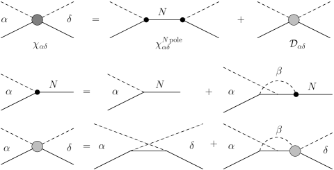
Figure 1: Graphical representation of Eqs. (10), (11) and (12) (from top to bottom).

Since we assume that the nucleon in (1) is an exact solution of the Hamiltonian and therefore consists of the pion and $\sigma$ clouds, the vertex $\bar{V}_{\alpha N}$ in (11) is a modification of the ground-states meson amplitudes such that its off-shell value goes to zero as $W$ approaches $m_{N}$:

$$\bar{V}_{\alpha N}(k)={(W-m_{N})V_{\alpha N}(k)\over\omega_{\alpha}(k)+E_{\alpha}(k)-m_{N}}\,.$$ (13)

Finally

$$c_{\alpha N}=-{\mathcal{V}_{\alpha N}(k)\over\lambda_{N}(W)}\,,$$ (14)

where

$$\lambda_{N}(W)=W-m_{N}+\sum_{\beta}\int\mathrm{d}k\;{\mathcal{V}_{\beta N}(k)\bar{V}_{\beta N}(k)\over\omega_{\beta}(k)+E_{\beta}(k)-W}\,.$$ (15)

Note that due to (13) the self-energy term vanishes as $W\to m_{N}$.

Since the kernel (7) is separable, Eqs. (11) and (12) can be exactly solved with the ansaetze

$$\mathcal{V}_{\alpha N}(k)=\bar{V}_{\alpha N}(k)+\sum_{\beta i}x^{\alpha}_{\beta i}\,\varphi^{\alpha}_{\beta i}(k)$$ (16)

and

$$\mathcal{D}_{\alpha\delta}(k,k_{\delta})=\mathcal{K}_{\alpha\delta}(k,k_{\delta})+\sum_{\beta i}z^{\alpha\delta}_{\beta i}\,\varphi^{\alpha}_{\beta i}(k)\,.$$ (17)

This leads to a set of linear algebraic equations for the coefficients $x$ and $z$:

$$x^{\alpha}_{\beta i}+\sum_{\gamma j}M^{\beta}_{\alpha i,\gamma j}\;x^{\beta}_{\gamma j} = b^{\beta}_{\alpha i}\,,$$ (18)

$$z^{\alpha\delta}_{\beta i}+\sum_{\gamma j}M^{\beta}_{\alpha i,\gamma j}\;z^{\beta\delta}_{\gamma j} = d^{\beta\delta}_{\alpha i}\,,$$ (19)

where

$$M^{\beta}_{\alpha i,\gamma j} = -\int\mathrm{d}k\;{\xi^{\beta}_{\alpha i}(k)\varphi^{\beta}_{\gamma j}(k)\over\omega_{\beta}(k)+E_{\beta}(k)-W}\,,$$ (20)

$$b^{\beta}_{\alpha i} = \int\mathrm{d}k\;{\bar{V}_{\beta N}(k)\xi^{\beta}_{\alpha i}(k)\over\omega_{\beta}(k)+E_{\beta}(k)-W}\,,$$

$$d^{\beta\delta}_{\alpha i} = \int\mathrm{d}k\;{\mathcal{K}_{\beta\delta}(k,k_{\delta})\xi^{\beta}_{\alpha i}(k)\over\omega_{\beta}(k)+E_{\beta}(k)-W}\,.$$

Figure 2: Graphical representation of $M^{\beta}_{\alpha i,\gamma j}$: $M_{\alpha}$ and $B_{\alpha}$ denote respectively the meson ($\pi$ or $\sigma$) and baryon ($N$ or $\Delta$) in channel $\alpha$.

The meaning of the indices in the matrix ${\sf M}=[M]^{\beta}_{\alpha i,\gamma j}$ is explained in Fig. 2. Introducing ${\sf A}={\sf I}+{\sf M}$, (18) can be written as ${\sf A}\bm{x}=\bm{b}$ or, in terms of components, as

$$\sum_{\gamma j}A^{\beta\eta}_{\alpha i,\gamma j}\;x^{\eta}_{\gamma j}=b^{\beta}_{\alpha i}\,,$$ (21)

where

$$A^{\beta\eta}_{\alpha i,\gamma j}=I^{\beta\eta}_{\alpha i,\gamma j}+\delta_{\beta,\eta}M^{\beta}_{\alpha i,\gamma j}\,,\qquad I^{\beta\eta}_{\alpha i,\gamma j}=\delta_{\alpha,\eta}\delta_{\beta,\gamma}\delta_{i,j}\,.$$

The set (19) for the $z$ parameters differs only in the right-hand side. The structure of A for our choice of channels is displayed in the Appendix.

In order to analyze the behaviour of the kernel we perform the singular value decomposition of A,

$${\sf A}={\sf U}{\sf W}{\sf V}^{T}\,,$$ (22)

where U and V are orthogonal matrices and W is a diagonal matrix. Since ${\sf A}^{-1}={\sf V}{\sf W}^{-1}{\sf U}^{T}$, the solution for $x$ can be written as

$$\bm{x}={\sf A}^{-1}\bm{b}\,,\qquad x_{p}=\sum_{r=1}^{\mathrm{dim}({\sf A})}{1\over w_{r}}\left(\sum_{q}U_{rq}b_{q}\right)V_{pr}\,.$$ (23)

We have introduced common indices $p,q,r$ numbering possible combinations of the two channels indices (e.g. $\alpha$ and $\beta$) and the index of the intermediate state ($i$); in the present case $\mathrm{dim}({\sf A})=13$.

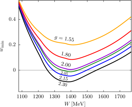
Figure 3: The behaviour of the lowest eigenvalue $w_{\mathrm{min}}$ as a function of $W$ for $\mu_{\sigma}=\Gamma_{\sigma}=600$ MeV for coupling constant $g$ from 1.55 to 2.3.

For weak couplings $g$ the eigenvalues $w_{r}$ remain close to 1; increasing $g$, one of the eigenvalues denoted $w_{\mathrm{min}}$ becomes smaller while the others stay close to 1. Figure 3 shows that the minimum is reached around $W=1400$ MeV almost independently of $g$; this value of the invariant mass is also insensitive to the choice of the Breit-Wigner mass and width of the $\sigma$ meson. The solution in the energy range from $W\approx 1300$ MeV to 1600 MeV is therefore dominated by the lowest eigenvector of A. Around $g=2$, $w_{\mathrm{min}}$ touches zero and beyond this (critical) value it crosses zero twice, at $W_{1}$ and $W_{2}$. At these two energies, a nontrivial solution of the homogeneous equation appears, signaling the emergence of a (quasi)-bound state. The corresponding eigenvector changes little with $W$ and stays almost constant for $1300~{}\mathrm{MeV}<W<1600~{}\mathrm{MeV}$. This remains true even for $g$ smaller than the critical value, except that the $\sigma N$ component is less strong. (See Fig. 4.) As we shall justify in the following we can identify the corresponding state as the dynamically generated state.

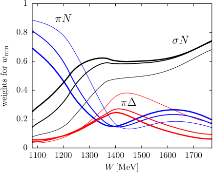
Figure 4: The weights of the $\pi N$, $\pi\Delta$ and $\sigma N$ components of the eigenvector belonging to the lowest eigenvalue $w_{\mathrm{min}}$ for $g=2.3$ (thick lines), $g=2.0$ (medium lines) and $g=1.55$ (thin lines), and $\mu_{\sigma}=\Gamma_{\sigma}=600$ MeV.

Let us consider how the lowest eigenvalue influences the behaviour of the $K$ matrix, which has the form

$$K_{\alpha\beta}=\pi\,\mathcal{N}_{\alpha}\mathcal{N}_{\beta}\left[{{\cal V}_{\alpha N}{\cal V}_{\beta N}\over\lambda_{N}(W)}+{\cal D}_{\alpha\beta}\right]\,.$$ (24)

When $w_{\mathrm{min}}$ approaches zero, ${\cal V}_{\alpha N}$ and ${\cal D}_{\alpha\beta}$ are dominated by the dynamically generated state and both quantities become proportional to $w_{\mathrm{min}}^{-1}$; the same is true also for $\lambda_{N}(W)$ (see Eq. (15)). As a result, the $K$ matrix also behaves like $w_{\mathrm{min}}^{-1}$ and therefore possesses the pole at those $W$ where $w_{\mathrm{min}}$ crosses zero. Let us note that while the A is not symmetric, the resulting $K$ matrix (24) is symmetric (and real), which guarantees the unitarity of the $S$ matrix.

The $T$ matrix is obtained by solving the Heitler equation $T=K+\mathrm{i}KT$. The influence of the dynamically generated state on the $T$ matrix is best visualized by observing the behaviour of the imaginary part of $T$ (Fig. 5) as we increase $g$. For $g$ below the critical value (but not too small) there is a single bump roughly where $w_{\mathrm{min}}$ reaches its minimum. For $g=2.05$ we have two poles in the $K$ matrix and two peaks in Im$T$. As we increase $g$, the lower peak gets narrower and weaker and disappears at the location of the two pion threshold. The upper peak moves to higher $W$ and becomes wider.

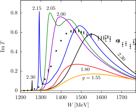
Figure 5: The imaginary part of the $T$ matrix for $g$ from 1.55 to 2.3 and $\mu_{\sigma}=\Gamma_{\sigma}=600$ MeV.

Table 1: $S$-matrix pole position and modulus for $g$ from 1.8 to 2.15; at $g=2.15$ the width and modulus of the lower resonance can not be reliably determined. The PDG values are taken from PDG .

$g$	Re$W_{p}$	$-2{\rm Im}W_{p}$	$|r|$	$\vartheta$
	[MeV]	[MeV]
PDG	1370	180	46	$-90^{\circ}$
1.55	1407	207	12.6	$-101^{\circ}$
1.80	1395	148	10.5	$-79^{\circ}$
1.95	1382	129	17.1	$-59^{\circ}$
2.00	1375	111	34.0	$-44^{\circ}$
2.05	1331	44	7.3	$-62^{\circ}$
	1438	147	18.6	$-17^{\circ}$
2.15	1291
	1476	166	30.1	$-27^{\circ}$

From scattering amplitudes we can use the Laurent-Pietarinen expansion L+P2013 ; L+P2014 ; L+P2015 ; L+P2014a to extract the information about the $S$-matrix poles shown in Table 1 which offers a deeper insight into the mechanism of resonance formation. Notice that the pole in the $S$ matrix emerges already before the critical value of $g$ is reached. This means that it is not necessary that the kernel in the Lippmann-Schwinger equation (4) becomes singular in order to produce a resonance — or, equivalently, it is not necessary that the $K$ matrix possesses a pole in the vicinity of the resonance. The mass of the $S$-matrix pole, Re$W_{p}$, is close to the mass of the Roper pole extracted from the data while the width and the modulus are relatively too small. Above the critical $g$, where the $K$ matrix acquires two poles on the real axis, two poles appear also in the complex plane with the upper pole gaining strength as it moves toward higher $W$ while the opposite is true for the lower one as it moves toward lower $W$.

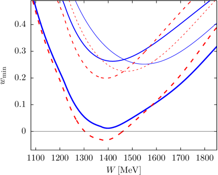
Figure 6: The lowest eigenvalue of A as a function of $W$ for $g=2.0$, $\mu_{\sigma}=\Gamma_{\sigma}=600$ MeV (blue) and $\mu_{\sigma}=\Gamma_{\sigma}=500$ MeV (red); the thick solid lines correspond to the full calculation, medium lines to the system without $\Delta$, and thin lines to the $\sigma N$ system alone.

Despite its simplicity our model is able to predict correctly the mass of the Roper resonance. On the other hand, it is precisely this simplicity that enables us to study and reveal the parameters that determine the resonant energy. At first glance it might seem that it is the mass of the $\Delta$ that most strongly influences the position of the resonance since Re$W_{p}$ almost coincides with the $\pi\Delta$ threshold. However, increasing/decreasing the (Breit-Wigner) mass of the $\Delta$ turns out to have very little effect on the position. This remains true even if we remove the $\pi\Delta$ channel and eliminate completely the $\Delta$ intermediate state from the loops. The effect can be best observed through the behaviour of the lowest eigenvalue of the matrix A, $w_{\mathrm{min}}$, as a function of $W$, for which we have shown that the position of its minimum coincides with the mass of the resonance pole even when $w_{\mathrm{min}}$ does not touch or cross zero. In Fig. 6 one sees that the shape of $w_{\mathrm{min}}(W)$ changes little if the $\Delta$ is removed from the calculation: in particular the position of the minimum remains almost unchanged. In fact, by increasing the coupling strength $g$ in the case of only two channels, the two curves would almost coincide. The conclusion is further supported by analysing the parameters of the $S$-matrix pole in Table 2: for $g=2.00$ the mass remains close to the corresponding three-channel case in Table 1, while its width is increased and the modulus decreased, in agreement with the tendency shown in Table 1 when reducing the coupling strength in the three-channel case. Similarly, for a larger value of $g=2.25$ the mass and the width are reduced and the modulus increased.

Table 2: Same as table 1 for the case without the $\pi\Delta$ channel.

$g$	Re$W_{p}$	$-2{\rm Im}W_{p}$	$|r|$	$\vartheta$
	[MeV]	[MeV]
PDG	1370	180	46	$-90^{\circ}$
2.00	1342	285	18.8	$-11^{\circ}$
2.25	1329	204	28.5	$-125^{\circ}$

Finally, our model allows us to switch off the $\pi N$ interaction and study the $\sigma N$ system alone. In this case the minimum of $w_{\mathrm{min}}(W)$ is shifted higher in $W$, slightly above the $\sigma N$ threshold (for the nominal mass of the $\sigma$ meson), see Fig. 6. Our model therefore proposes the following scenario for the formation of the Roper resonance: the $\sigma N$ interaction is responsible to generate a quasi-bound state close to the $\sigma N$ threshold; by coupling this state to the $\pi N$ state, the energy of the quasi-bound state is reduced to around 1400 MeV; furthermore, the coupling to the $\pi\Delta$ system makes the system more bound (or, alternatively, produces the quasi-bound state for weaker couplings) but does not change its position. While the position of the first state (in the $\sigma N$ channel alone) still strongly depends on the (nominal) $\sigma$ mass, the final state is only weakly sensitive to the variation of the $\sigma$ mass.

If we remove the nucleon pole and keep only the background term (see Fig. 7) we encounter a similar situation as discussed in Ref. Roenchen13 . As mentioned in relation with Eq. (24) both the (positive) non-pole contribution to the $K$-matrix and the (negative) nucleon-pole contribution are proportional to the inverse of the lowest eigenvalue of A which reaches its minimum at around 1400 MeV. Consequently the $K$-matrix elements of both parts acquire very large values which almost cancel in the resulting $K$ matrix. This cancellation is reflected in a high sensitivity of the Im$T_{\pi N\,\pi N}$ to small variations of the model parameters as can be seen in Fig. 7. This is not the case with the Im$T_{\pi N\,\pi N}$ calculated from the non-pole part alone; it rises quickly towards unity (as indicated by the elastic matrix element alone). Above the two-pion threshold, the other two channels start to contribute, resulting in a gradual decrease of its value. The resulting maximum has therefore no physical meaning whatsoever.

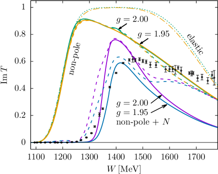
Figure 7: The imaginary part of the $T_{\pi N\,\pi N}$ amplitude; the non-pole contribution is shown separately as well as the contribution from the lowest state of the A matrix (dashed lines) for $g=2.00$ and $g=1.95$.

Let us mention that the mechanism of the resonance formation carries some similarities with the model considered by the Coimbra-Ljubljana group Pedro using the quark-level Chromodielectric Model which incorporates the linear $\sigma$ model with an additional dynamical (chromodielectric) field responsible for the quark binding. The stability condition amounts to solving the Klein-Gordon equation for the $\sigma$-meson modes. The lowest mode turns out to be some 100 MeV below the $\sigma N$ threshold, similarly as in the present case. In that calculation, the $\sigma$ mass was higher (i.e. 700 MeV and 1200 MeV) than in our case and the corresponding bound state was above the $2s$ quark excitation; consequently, the Roper resonance was interpreted as a linear superposition of the dominant quark excitation and a quasi-bound $\sigma N$ state.

IV Including a three-quark resonant state

We now include in (1) a three-quark configuration with one quark excited to the $2s$ state. The coupling of this state to $\pi N$ and $\pi\Delta$ is calculated in the underlying quark model, while the $\sigma NR$ coupling is assumed to be equal to the $\sigma NN$ coupling.

The meson amplitude (proportional to the $K$ matrix) now takes the form

$$\chi_{\alpha\delta}(k,k_{\delta})=c_{\delta N}{\cal V}_{\alpha N}(k)+c_{\delta R}{\cal V}_{\alpha R}(k)+{\cal D}_{\alpha\delta}(k,k_{\delta})\,,$$ (25)

with ${\cal V}_{\alpha N}$ and ${\cal D}_{\alpha\delta}(k,k_{\delta})$ satisfying (11) and (12), respectively, and

$$\mathcal{V}_{\alpha R}(k)={V}_{\alpha R}(k)+\sum_{\beta}\int\mathrm{d}k^{\prime}\;{\mathcal{K}_{\alpha\beta}(k,k^{\prime})\mathcal{V}_{\beta R}(k^{\prime})\over\omega_{\beta}(k^{\prime})+E_{\beta}(k^{\prime})-W}\,.$$ (26)

The nucleon and the three-quark ($3q$) resonant state mix through meson loops, yielding the following set of equations for $c_{\alpha N}$ and $c_{\alpha R}$:

$$\begin{array}[]{lll}G_{RR}(W)\,c_{\alpha R}&+\;G_{RN}(W)\,c_{\alpha N}&=\mathcal{V}_{\alpha R}(k_{\alpha})\,,\\ G_{NR}(W)\,c_{\alpha R}&+\;G_{NN}(W)\,c_{\alpha N}&=\mathcal{V}_{\alpha N}(k_{\alpha})\,,\end{array}$$ (27)

with $G_{NN}$ given in (15), and

$$G_{RR}(W) = W-m_{R}^{0}+\sum_{\beta}\int\mathrm{d}k\;{\mathcal{V}_{\beta R}(k){V}_{\beta R}(k)\over\omega_{\beta}(k)+E_{\beta}(k)-W}\,,$$

$$G_{NR}(W) = G_{RN}(W)=\sum_{\beta}\int\mathrm{d}k\;{\mathcal{V}_{\beta N}(k){V}_{\beta R}(k)\over\omega_{\beta}(k)+E_{\beta}(k)-W}\,,$$

were $m_{R}^{0}$ is the bare mass of the $3q$ resonant state.

Let ${\sf U}$ denote the unitary transformation that diagonalises the ${\sf G}$ matrix in the left-hand side of (27):

$${\sf U}{\sf G}{\sf U}^{T}=\hbox{diag}[\lambda_{R}(W),\lambda_{N}(W)]\,.$$ (28)

The resonance part of the $K$ matrix can then be cast in the form

$$K_{\alpha\beta}^{\mathrm{res}}=\pi\,\mathcal{N}_{\alpha}\mathcal{N}_{\beta}\left[{\widehat{\cal V}_{\alpha R}\widehat{\cal V}_{\beta R}\over\lambda_{R}(W)}+{\widehat{\cal V}_{\alpha N}\widehat{\cal V}_{\beta N}\over\lambda_{N}(W)}\right]\,,$$ (29)

where

$$\widehat{\cal V}_{\alpha R}=u_{RR}{\cal V}_{\alpha R}+u_{RN}{\cal V}_{\alpha N}\,,\quad\widehat{\cal V}_{\beta N}=u_{NR}{\cal V}_{\beta R}+u_{NN}{\cal V}_{\beta N}\,,$$ (30)

and $u$’s denote the matrix elements of ${\sf U}$. The $3q$ resonant state contains an admixture of the ground state and vice versa. Due to the particular ansatz for the meson amplitude (13), $\widehat{\cal V}_{\beta N}$ vanishes at the nucleon pole ($W=m_{N}$). Also, due to this ansatz, one of the zeros of $\lambda_{N}(W)$ is always at the nucleon mass, $m_{N}$.

The set of equations (18) and (19) is supplemented by an equation for $\mathcal{V}_{\alpha R}(k)$ which has the same form as (18) with $V_{\beta R}$ replacing $\bar{V}_{\beta N}$ on the right. It is important to notice that the matrices M, given by (20), and ${\sf A}={\sf I}+{\sf M}$ remain unchanged with respect to the case with no $3q$ resonant state and hence for $g$ larger than the critical $g$, two poles in the $K$ matrix appear at the same energies as in the case without the $3q$ resonant state; other poles appear at the zeros of $\lambda_{N}$ and $\lambda_{R}$.

The free parameter of our model is the bare mass of the $3q$ resonant state, $m_{R}^{0}$. In our calculation we do not fix it but adjust it in such a way that one of the zeros of $\lambda_{R}(W)$ (poles of the $K$ matrix) is kept at the prescribed value $m_{R}$. In our analysis we therefore study the influence of $m_{R}$ on the behaviour of the scattering amplitudes. A similar model of the P11 scattering has been studied in EPJ2008 ; EPJ2009 as well as in EPJ2016 . In these calculations we kept $m_{R}$ close to the Breit-Wigner mass and included the $\sigma N$ channel only at the tree level (ignoring the $\sigma$-meson loops).

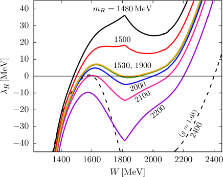
Figure 8: $\lambda_{R}(W)$ for masses of the $3q$ resonant state $m_{R}$ from 1480 MeV to 2200 MeV and $g=1.55$, $\mu_{\sigma}=\Gamma_{\sigma}=600$ MeV.

For small $g$, the poles of the $K$ matrix are only at $m_{N}$ and $m_{R}$, while for larger $g$, $\lambda_{R}(W)$ may develop additional zeros. A typical behaviour of $\lambda_{R}(W)$ for different $m_{R}$ is displayed in Fig. 8. Below $m_{R}\approx 1520$ MeV, the zero crossing at $m_{R}$ yields the only pole in the $K$ matrix; above this value, two additional poles appear, for smaller $m_{R}$ at $W$ higher than $m_{R}$, while for $m_{R}>1600$ MeV at least one of the additional $K$-matrix poles emerges below $m_{R}$. It is important to stress that these two additional poles are not directly related to the zeros of $w_{\mathrm{min}}$ discussed in the previous section since the value of $g$ is smaller than the critical value; nonetheless, the emergence of these two poles is a consequence of the dynamical state whose effect is enhanced by the presence of the $3q$ resonant state. The most striking observation is that $\lambda_{R}(W)$ has very similar behaviour for $m_{R}=1530$ MeV as for $m_{R}=1900$ MeV even though the origin of the lowest $K$-matrix pole is different. The resulting poles in the $S$ matrix are displayed in Table 3. The position and the residue of the Roper pole are well reproduced for $g=1.55$ and $\mu_{\sigma}=\Gamma_{\sigma}=600$ MeV for a wide range of values of $m_{R}$ between 1520 MeV and 2000 MeV, and remain close to the PDG values even if we considerably alter the values of $g$. The results are also rather insensitive to a simultaneous reduction of the $\sigma$ mass and $g$.

Table 3: $S$-matrix pole positions for various values of $g$, $m_{R}$ and $\mu_{\sigma}$ ($\Gamma_{\sigma}=\mu_{\sigma}$).

$m_{R}$	$\mu_{\sigma}$	$g$	Re$W_{p}$	$-2{\rm Im}W_{p}$	$|r|$	$\vartheta$
[MeV]	[MeV]		[MeV]	[MeV]
PDG			1370	180	46	$-90^{\circ}$
2000	600	1.55	1368	180	48.0	$-87^{\circ}$
2000	600	1.70	1361	156	41.9	$-77^{\circ}$
1530	600	1.55	1367	180	47.5	$-86^{\circ}$
2400	600	1.68	1370	177	42.6	$-87^{\circ}$
3000	600	1.85	1364	188	37.7	$-98^{\circ}$
2000	500	1.43	1369	172	40.2	$-82^{\circ}$
1530	500	1.36	1365	174	43.6	$-82^{\circ}$

The fact that the position of the pole remains so stable even if we considerably change the parameters of the model clearly shows that the position is determined by the dynamical state discussed in the previous section rather than the value of $m_{R}$. It almost coincides with the minimum of the lowest eigenvalue $w_{\mathrm{min}}$ of the matrix A. Here we encounter a similar situation as in the previous section, namely, that the $S$-matrix pole appears where $w_{\mathrm{min}}$ (or, equivalently, $\lambda_{R}$) only approaches zero, i.e. without producing poles in the $K$ matrix. However, the dynamical state alone yields too small values for the width and the residuum of the pole; these observables are brought closer to the values reported by PDG by inclusion of a $3q$ resonant state. The interplay of these two states is displayed in Fig. 10 showing the behaviour of Im$T(W)$ for typical values of $g$. For intermediate values of $g$ which best reproduce the properties of the resonance when the $3q$ resonant state in turned on, the effect of the dynamically generated state is still weak; for larger values of $g$ this state dominates and the influence of the $3q$ resonant state is almost invisible.

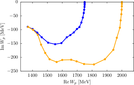
Figure 9: Evolution of the Roper pole as the interaction strength is gradually switched on for two bare masses of the three-quark configuration, 1750 MeV and 2000 MeV.

This conclusion is further strengthened by observing the evolution of the Roper resonance pole as the interaction strength of the $\sigma$ as well as the pion interactions is gradually switched on (see Fig. 9), similarly as in Ref. Sato-Lee10a . In our approach we fix the position of the $K$-matrix pole, which in the limit of zero coupling coincides with the energy of the bare three-quark state. We choose two different values, 1750 MeV and 2000 MeV, which are in agreement with the prediction of the continuum approach to the baryon bound-state, e.g. as in Ref. Segovia15 . As in the work of the EBAC group the continuous trajectory from the bare state shows that the resonance indeed originates from the bare state; nonetheless, the fact that the trajectories from two different bare states meet almost at the same point at the value of $W$ where the dynamically generated “molecular” state attains its lowest value, confirms the notion that both states (mechanisms) contribute to the formation of the Roper resonance. This is true even if the $\sigma$ coupling is substantially weaker compared to the situation treated in the previous section.

The mixing of the ground state to the $3q$ resonant state through the meson loops is measured by the squared matrix element $u^{2}_{RN}$ of the ${\sf U}$ matrix introduced in Eq. (28). The value of $u^{2}_{RN}$ strongly depends on $W$ and reaches its maximum near the mass of the resonance pole. For the typical value of $g=1.55$ it comes close to 50 % which means that the probability of finding the excited three-quark configuration in the $3q$ resonant state is further reduced with respect to the pure quark model.

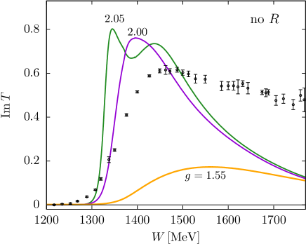
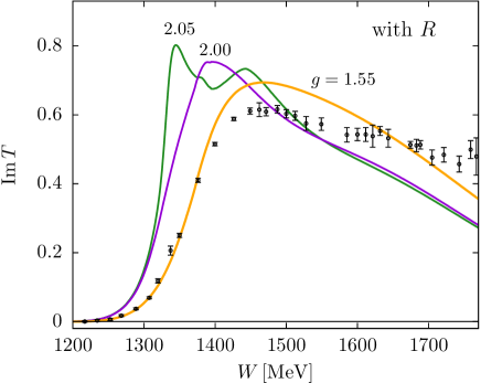
Figure 10: Im$T(W)$ for $\mu_{\sigma}=600$ MeV when the $3q$ resonant state with $m_{R}=2000$ MeV is turned off (left) and on (right).

Our coupled channel approach is similar to the pioneering approach of Krehl et al. Krehl using a coupled-channel meson exchange model and that of the Adelaide group using Hamiltonian effective field theory. They both solve the Lippmann-Schwinger equation for the $T$ matrix which has an analogous form as our $K$ matrix consisting of the resonant part and the background part. Krehl et al. Krehl were the first to notice that the resonance can be formed by using only the $\pi N$ and the $\sigma N$ channels, which has been confirmed also in our calculation in the previous section. Our results are consistent with those obtained by the Adelaide group. The advantage of our approach is that it uses a smaller number of free parameters since it relates the pion couplings to different baryons through the underlying quark model and the calculations in other partial waves. Furthermore, we treat two (or more) baryon states simultaneously and thus studying the interplay of the nucleon and the Roper degrees of freedom. The relevance of the $N+\sigma$ admixture to the excited $3q$ configuration has been also realized in the calculation of electro-production of the Roper resonance in Refs. tubingen11 ; tubingen14 .

V Conclusion

We have developed a simplified model including the $\pi N$, $\pi\Delta$ and $\sigma N$ channels to study the formation of the Roper resonance in the presence of a three-quark resonant state or in its absence. The number of model parameters is kept as small as possible and only the $u$-channel exchange as the sole background process is considered. The Laurent-Pietarinen expansion has been used to extract the $S$-matrix resonance-pole parameters. Despite the simplicity of the model, the properties of the Roper resonance are well reproduced in the intermediate coupling regime in which both the dynamically generated state as well as the three-quark resonant state contribute.

We have been able to pin down one particular state with $\pi N$, $\pi\Delta$ and $\sigma N$ components which dominates the scattering amplitudes between $W\approx 1300$ MeV and $W\approx 1500$ MeV and is responsible for the dynamical generation of the resonance. Its mass lies very close to the mass of the Roper pole and is very insensitive to rather large variations of the model parameters and even to the removal of the $\pi\Delta$ channel. We infer that this very state determines the mass of the Roper resonance, except in the case when the three-quark resonant state is included with the mass equal to or below 1500 MeV. Nonetheless, it appears that the dynamically generated state does not describe adequately the resonance properties; in the intermediate coupling regime it produces only a weak $S$-matrix pole in the complex plane which evolves towards the PDG values for the position and the residuum only upon inclusion of the three-quark state. This evolution is rather insensitive to the mass of the three-quark state which may be as large as 2000 MeV. In view of the difficulties in the quark model to explain the ordering of single-particle states in which the $2s$ state would lie lower than the $1p$ state, as well as the recent results of the lattice calculations lang16 ; kiratidis17 which have not found a sizable three-quark component below 1.65 GeV and 2.0 GeV, respectively, the presented model appears to rule out the existence of a three-quark resonant state around or below 1500 MeV. It favours the picture in which the mass of the $S$-matrix pole is determined by the energy of the dynamically generated state while its width and modulus are strongly influenced by the three-quark resonant state.

Though the description of the Roper resonance as a purely dynamically generated phenomenon could be further refined by including a richer set of backgrounds, we can not find a convincing reason to a priori exclude its genuine three-quark component. From our viewpoint this appears to be the simplest addition needed to reach satisfactory agreement with resonance properties extracted from the data.

*

Appendix A Structure of the A matrix

The A matrix elements are of the form $A^{\beta\eta}_{\alpha i,\gamma j}$, and the vectors are labeled by the three indices $\beta\alpha i$. Below $N,\Delta$ and $\sigma$ are a shorthand notation for the $\pi N,\pi\Delta$ and $\sigma N$ channels, while $i$ and $j$ denote the intermediate baryon, $N$ or $\Delta$ (see Fig. 2). The index $i$ ($j$) is dropped in those matrix elements that involve the $\sigma N$ channel since the $\sigma$ vertex preserves spin/isospin and only $N$ or $\Delta$ is present. The dimension of the first two submatrices is 5, while that of the third one is 3 resulting in $\mathrm{dim}({\sf A})=13$.

$$\begin{array}[]{|c|ccc|ccc|ccc|}\hline\cr\lower 1.0pt\hbox{${\beta\alpha i}$}\hbox{\LARGE$\diagdown$}\kern-3.0pt\raise 4.0pt\hbox{${\eta\gamma j}$}&NNj&N\Delta j&N\sigma N&\Delta Nj&\Delta\Delta j&\Delta\sigma\Delta&\sigma NN&\sigma\Delta\Delta&\sigma\sigma N\\ \hline\cr\vrule width=0.0pt,height=12.0pt,depth=5.0ptNNi&\delta_{i,j}+M^{N}_{Ni,Nj}&M^{N}_{Ni,\Delta j}&M^{N}_{Ni,\sigma}&0&0&0&0&0&0\\ \vrule width=0.0pt,height=12.0pt,depth=5.0ptN\Delta i&M^{N}_{\Delta i,Nj}&M^{N}_{\Delta i,\Delta j}&M^{N}_{\Delta i,\sigma}&\delta_{i,j}&0&0&0&0&0\\ \vrule width=0.0pt,height=12.0pt,depth=5.0ptN\sigma N&M^{N}_{\sigma,Nj}&M^{N}_{\sigma,\Delta j}&M^{N}_{\sigma,\sigma}&0&0&0&1&0&0\\ \hline\cr\vrule width=0.0pt,height=12.0pt,depth=5.0pt\Delta Ni&0&\delta_{i,j}&0&M^{\Delta}_{Ni,Nj}&M^{\Delta}_{Ni,\Delta j}&M^{\Delta}_{Ni,\sigma}&0&0&0\\ \vrule width=0.0pt,height=12.0pt,depth=5.0pt\Delta\Delta i&0&0&0&M^{\Delta}_{\Delta i,Nj}&\delta_{i,j}+M^{\Delta}_{\Delta i,\Delta j}&M^{\Delta}_{\Delta i,\sigma}&0&0&0\\ \vrule width=0.0pt,height=12.0pt,depth=5.0pt\Delta\sigma\Delta&0&0&0&M^{\Delta}_{\sigma,Nj}&M^{\Delta}_{\sigma,\Delta j}&M^{\Delta}_{\sigma,\sigma}&0&1&0\\ \hline\cr\vrule width=0.0pt,height=12.0pt,depth=5.0pt\sigma NN&0&0&1&0&0&0&M^{\sigma}_{N,N}&M^{\sigma}_{N,\Delta}&M^{\sigma}_{N,\sigma}\\ \vrule width=0.0pt,height=12.0pt,depth=5.0pt\sigma\Delta\Delta&0&0&0&0&0&1&M^{\sigma}_{\Delta,N}&M^{\sigma}_{\Delta,\Delta}&M^{\sigma}_{\Delta,\sigma}\\ \vrule width=0.0pt,height=12.0pt,depth=5.0pt\sigma\sigma N&0&0&0&0&0&0&M^{\sigma}_{\sigma,N}&M^{\sigma}_{\sigma,\Delta}&1+M^{\sigma}_{\sigma,\sigma}\\ \hline\cr\end{array}$$

References

- (1) L. D. Roper, Phys. Rev. Lett. 12, 137 (1964).
- (2) V. Shklyar, H. Lenske, U. Mosel, Phys. Rev. C 87, 015201 (2013).
- (3) A. V. Anisovich, R. Beck, E. Klempt, V. A. Nikonov, A. V. Sarantsev, U. Thoma, Eur. Phys. A 48, 15 (2012).
- (4) R. A. Arndt, W. J. Briscoe, I. I. Strakovsky, R. L. Workman, Phys. Rev. C 74, 045205 (2006).
- (5) S. Capstick, Phys. Rev. D 46, 2864 (1992); S. Capstick and B. D. Keister, Phys. Rev. D 51, 3598 (1995).
- (6) H. J. Weber, Phys. Rev. C 41, 2783 (1990).
- (7) F. Cardarelli, E. Pace, G. Salmè and S. Simula, Phys. Lett. B 397, 13 (1997).
- (8) B. Juliá-Díaz, D. O. Riska, F. Coester, Phys. Rev. C 69, 035212 (2004).
- (9) I. G. Aznauryan, Phys. Rev. C 76, 025212 (2007).
- (10) Zhenping Li, Volker Burkert, and Zhujun Li, Phys. Rev. D 46, 70 (1992).
- (11) W. Broniowski, T. D. Cohen and M. K. Banerjee, Phys. Lett. B 187, 229 (1987).
- (12) O. Krehl, C. Hanhart, S. Krewald, and J. Speth, Phys. Rev. C 62, 025207 (2000).
- (13) D. Rönchen et al., Eur. Phys. J. A 49, 44 (2013).
- (14) J. Segovia et al., Phys. Rev. Lett. 115, 171801 (2015).
- (15) E. Hernández, E. Oset, M. J. Vicente Vacas, Phys. Rev. C 66, 065201 (2002).
- (16) P. Alberto, M. Fiolhais, B. Golli, and J. Marques, Phys. Lett. B 523, 273 (2001)
- (17) B. Golli and S. Širca, Eur. Phys. J. A 38, 271 (2008).
- (18) B. Golli, S. Širca, and M. Fiolhais, Eur. Phys. J. A 42, 185 (2009).
- (19) F. Cano and P. González, Phys. Lett. B 431, 270 (1998).
- (20) Y. B. Dong, K. Shimizu, A. Faessler, and A. J. Buchmann, Phys. Rev. C 60, 035203 (1999).
- (21) K. Bermuth, D. Drechsel and L. Tiator, Phys. Rev. D 37, 89 (1988).
- (22) I. T. Obukhovsky, A. Faessler, D. K. Fedorov, T. Gutsche, V. E. Lyubovitskij, Phys. Rev. D 84 014004 (2011).
- (23) I. T. Obukhovsky, A. Faessler, T. Gutsche, V. E. Lyubovitskij, Phys. Rev. D 89 014032 (2014).
- (24) L. Tiator, M. Vanderhaeghen, Phys. Lett. B 672, 344 (2009).
- (25) N. Suzuki, B. Juliá-Díaz, H. Kamano, T.-S. H. Lee, A. Matsuyama, and T. Sato, Phys. Rev. Lett. 104, 042302 (2010).
- (26) H. Kamano, S. X. Nakamura, T.-S. H. Lee, and T. Sato Phys. Rev. C 81, 065207 (2010).
- (27) D. Leinweber et al., JPS Conf. Proc. 10, 010011 (2016).
- (28) C. B. Lang, L. Leskovec, M. Padmanath, S. Prelovsek, Phys. Rev. D 95, 014510 (2017).
- (29) A. L. Kiratidis et al., Phys. Rev. D 95, 074507 (2017).
- (30) Zhan-Wei Liu, W. Kamleh, D. B. Leinweber, F. M. Stokes, A. W. Thomas, Jia-Jun Wu, Phys. Rev. D 95, 034034 (2017).
- (31) Jia-Jun Wu et al., arXiv:1703.10715 [nucl-th].
- (32) Jambul Gegelia, Ulf-G. Meißner, De-Liang Yao, Phys. Lett. B 760, 736 (2016).
- (33) B. Borasoy, P. C. Bruns, U.-G. Meißner, R. Lewis, Phys. Lett. B 641, 294 (2006).
- (34) A. W. Thomas, Adv. Nucl. Phys. 13, 1 (1984).
- (35) B. Golli, S. Širca, Eur. Phys. J. A 47, 61 (2011).
- (36) B. Golli, S. Širca, Eur. Phys. J. A 49, 111 (2013).
- (37) B. Golli, S. Širca, Eur. Phys. J. A 52, 279 (2016).
- (38) C. Patrignani et al. (Particle Data Group), Chin. Phys. C 40, 100001 (2016) and 2017 update.
- (39) A. Švarc, M. Hadžimehmedović, H. Osmanović, J. Stahov, L. Tiator, and R. L. Workman, Phys. Rev. C 88, 035206 (2013).
- (40) A. Švarc, M. Hadžimehmedović, R. Omerović, H. Osmanović, and J. Stahov, Phys. Rev. C 89, 045205 (2014).
- (41) A. Švarc, M. Hadžimehmedović, H. Osmanović, J. Stahov, and R. L. Workman, Phys. Rev. C 91, 015205 (2015).
- (42) A. Švarc, M. Hadžimehmedović, H. Osmanović, J. Stahov, L. Tiator, and R. L. Workman, Phys. Rev. C 89, 065208 (2014).