On-demand electron source with tunable energy distribution

Abstract

We propose a scheme to manipulate the electron-hole excitation in the voltage pulse electron source, which can be realized by a voltage-driven Ohmic contact connecting to a quantum hall edge channel. It has been known that the electron-hole excitation can be suppressed via Lorentzian pulses, leading to noiseless electron current. We show that, instead of the Lorentzian pulses, driven via the voltage pulse $V(t)=2\frac{\hbar}{e}\sqrt{\frac{\sqrt{3}}{\pi}k_{\rm B}T_{h}}\operatorname{arctanh}(\frac{t-t_{0}}{t_{0}})$ with duration $t_{0}$, the electron-hole excitation can be tuned so that the corresponding energy distribution of the emitted electrons follows the Fermi distribution with temperature $T_{\rm D}=\sqrt{T^{2}_{\rm S}+T^{2}_{\rm h}}$, with $T_{\rm S}$ being the electron temperature in the Ohmic contact. Such Fermi distribution can be established without introducing additional energy relaxation mechanism and can be detected via shot noise thermometry technique, making it helpful in the study of thermal transport and decoherence in mesoscopic system.

I INTRODUCTION

The on-demand coherent injection of single or few electrons in solid-state circuits is an important task in electron quantum optics, which focus on the manipulation of electrons in optics-like setups.Oliver et al. (1999); Henny et al. (1999); Bertoni et al. (2000); Ionicioiu et al. (2001); Ji et al. (2003); Bocquillon et al. (2014) The injection can be implemented simply by a voltage-pulse-driven Ohmic contact connecting to a quantum hall edge channel, which is usually referred as the voltage pulse electron source.Glattli and Roulleau (2017) The Ohmic contact serves as an electron reservoir, while the quantum hall edge channel serves as an electron waveguide. Driven by the voltage pulse applied on the Ohmic contact, electrons incoming from the reservoir can be injected on the Fermi sea of the edge channel, leading to the single-electron quasi-particle excitation propagating along the waveguide. However, additional electron-hole excitation can usually be created during the injection,Vanević et al. (2016) inducing charge current noise.

As far as the charge transport is concerned, it is desired to suppress the electron-hole excitation. In a series of seminal works, Levitov et al. have proposed that, driven by Lorentzian pulses with integer Faraday flux, integer electrons can be injected, while the accompanied electron-hole excitation can be suppressed, leading to a noiseless current flow.Lee and Levitov (1993, 1995); Keeling et al. (2006) This has been realized and extensively studied in the experiments reported in the group of D.C. Glattli.Dubois et al. (2013); Jullien et al. (2014); Glattli and Roulleau (2017) Later, Gabelli et al. further show that a similar suppression can be realized by using bi-harmonic voltage pulses.Gabelli et al. (2017) Besides, the existence of the electron-hole excitation can also be helpful in certain situation. Moskalets have demonstrated that, driven by the Lorentzian pulse with a half-integer flux, a zero-energy excitation with half-integer charge can be created in the driven Fermi sea at zero temperature, which cannot exist without the presence of electron-hole excitation.Moskalets (2016) These works demonstrate the possibility of manipulating electron-hole excitation via engineering the temporal profile of the voltage pulse.

In contrast, if the thermal transport is concerned,Schwab et al. (2000); Chiatti et al. (2006); Chen et al. (2009); Granger et al. (2009); Altimiras et al. (2010); Le Sueur et al. (2010); Venkatachalam et al. (2012); Jezouin et al. (2013) the electron-hole excitation are favorable, since they carry a finite amount of energy, while do not affect the average charge transport. In fact, a fully thermalized state at finite temperature can be regarded as the mixed state of certain electron-hole excitations, where the energy distribution follows the Fermi distribution, while the quantum coherence totally vanishes. If the electron-hole excitation can be manipulated via engineering the voltage pulse, it is then nature to ask: is it possible to tune the electron-hole excitation so that the corresponding state has exactly the same energy distribution of the fully thermalized state, while the quantum coherence is still preserved? Such a state will be helpful in the study of thermal transport and quantum decoherence processes in mesoscopic systems.

In this paper, we propose a scheme to create such a state by using the voltage pulse electron source. We find that, instead of Lorentzian pulses, driving via the voltage pulse with duration $t_{0}$, i.e., $t\in[0,t_{0}]$, which has the temporal profile

$$V(t) = 2\frac{\hbar}{e}\sqrt{\frac{\sqrt{3}}{\pi}k_{\rm B}T_{h}}\operatorname{arctanh}(\frac{t-t_{0}}{t_{0}}),$$ (1)

with $k_{\rm B}$ being the Boltzmann constant, electrons incoming from the reservoir at temperature $T_{\rm S}$ and chemical potential $\mu$ can be excited so that the corresponding outgoing electrons can have the time-averaged energy distribution as

$$f_{\rm D}(\omega) = \frac{1}{1+\exp[(\hbar\omega-\mu)/(k_{\rm B}T_{\rm D})]},$$ (2)

which is exactly a Fermi distribution at temperature

$$T_{\rm D} = \sqrt{T^{2}_{\rm S}+T^{2}_{\rm h}}.$$ (3)

Note that such Fermi distribution is obtained solely by coherent excitation via voltage pulses and no additional energy relaxation mechanism is needed. Hence the quantum coherence is still preserved for the state. Experimentally, it is possible to detect the energy distribution of the state via quantum-dot-based energy filter.Altimiras et al. (2010); Le Sueur et al. (2010) We further show that such state can also be detected in situ at the voltage pulse electron source via shot noise thermometry technique,Spietz et al. (2003) making it convenient in further experimentally studies.

The paper is organized as follows. In Sec. II, we present the model of the voltage pulse electron source and introduce the time-averaged energy distribution for the electrons. In Sec. III, we demonstrate how to manipulate the temporal profile of the pulse so that the time-averaged energy distribution of the emitted electrons follows the Fermi distribution we desired. In Sec. IV, we discuss the detection of the state via shot noise thermometry technique. We summarized in Sec. V.

II Model and Formalism

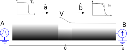
Figure 1: (Color online) Schematic of the voltage pulse source, composing of an one-dimensional quantum wire connecting two reservoirs A and B. Electrons are injected from the reservoir A by the time-dependent bias voltage $V$. The current and their fluctuation are detected in the reservoir B. The incoming(outgoing) wave-packet from(towards) the reservoir A(B) is represented by the operator $\hat{a}$($\hat{b}$). The energy distribution of the incoming (at temperature $T_{\rm S}$) and outgoing (at temperature $T_{\rm D}$) electron wave-packet are also illustrated. The 1D coordinates system is shown in the bottom of the figure.

The voltage pulse electron source can be modeled as an one-dimensional quantum wire connecting two reservoir A and B,Keeling et al. (2006) as illustrated in Fig. 1. The system is biased with a time-dependent voltage pulse $V(t)$ with duration $t_{0}$. The voltage drop is assumed to occur across a short interval at the center of the wire. If the voltage drop is spatially slow-varying on the scale of the Fermi wavelength $1/k_{\rm F}$, the electron in such system can be well-approximated as dispersionless Fermi systems with the corresponding single-particle Hamiltonian

$$H = -i\hbar(\pm v_{\rm F})\partial_{x}+eV(t)\theta(-x),$$ (4)

with $e$ being the charge of electron and $v_{\rm F}$ being the Fermi velocity. The sign $\pm$ corresponds to left- and right- going electrons, respectively. Without loss of generality, we focus on the right-going electron.

The field operator of the electron $\hat{\psi}(x,t)$ can be expressed as

$$\hat{\psi}(x,t) = \left\{\begin{tabular}[]{cc}$\hat{a}(t-x/v_{\rm F})e^{-i\phi(t)}$&,~{}$x<0$\\ $\hat{b}(t-x/v_{\rm F})$&,~{}$x>0$\\ \end{tabular}\right.,$$ (7)

with $\phi(t)=\frac{e}{\hbar}\int^{t}d\tau V(\tau)$ describing the effect of the voltage pulse $V(t)$. The Fermi operator $\hat{a}(t)$ and $\hat{b}(t)$ corresponds to the incoming and outgoing electron modes, respectively, which is also indicated in Fig. 1. They are related via the forward scattering phaseBlanter and Büttiker (2000); Keeling et al. (2006); Ivanov et al. (1997); Keeling et al. (2008)

$$\hat{b}(t) = \hat{a}(t)e^{-i\phi(t)},$$ (8)

which can be obtained by requiring the field operator $\hat{\psi}(x,t)$ is continuity at the boundary $x=0$.

Now we turn to discuss the energy distribution function of the incoming and outgoing electrons. Following previous works, the non-interacting electrons can be characterized by their one-body density matrix, which has the form of the first-order Glauber correlation function in the time-domain.Grenier et al. (2011); Haack et al. (2011, 2013) The correlation function for the incoming and outgoing electrons can be constructed as

$$G_{a}(t,t^{\prime}) = \left<\hat{a}^{\dagger}(t)\hat{a}(t^{\prime})\right>,$$

$$G_{b}(t,t^{\prime}) = \left<\hat{b}^{\dagger}(t)\hat{b}(t^{\prime})\right>,$$ (9)

respectively, where $\left<...\right>$ represents the thermal expectation over the reservoir degree of freedom.

For incoming electrons, which can be modelled as the stationary wave-packet emitted from the reservoir A at thermal equilibrium, the correlation function satisfies translation invariant in the time-domain, and hence only depends on the time difference $\tau=t-t^{\prime}$. The energy distribution function can be obtained through Fourier transformation, which has the form

$$f_{a}(\omega) = \int d\tau e^{i\omega\tau}G_{a}(t,t-\tau).$$ (10)

For reservoir A at temperature $T_{\rm S}$ and chemical potential $\mu$, the distribution $f_{a}(\omega)$ follows the Fermi distribution

$$f_{\rm S}(\omega) = \frac{1}{1+\exp[(\hbar\omega-\mu)/(k_{\rm B}T_{\rm S})]}.$$ (11)

In contrast, driven by the time-dependent potential $V(t)$, the outgoing electrons are described by the non-stationary wave-packet and the translation invariant of the correlation function is broken. In this situation, one can introduce the time-averaged energy distribution function over the time interval $t_{0}$, which can be written asLee and Levitov (1993, 1995); Kovrizhin and Chalker (2011, 2012); Moskalets (2014, 2016)

$$f_{\rm V}(\omega) = \frac{1}{t_{0}}\int^{t_{0}}_{0}\int^{t_{0}}_{0}dtdt^{\prime}e^{i\omega(t-t^{\prime})}G_{b}(t,t^{\prime}),$$ (12)

which can be measured experimentally by using quantum dot as an adjustable energy filter.Altimiras et al. (2010); Kovrizhin and Chalker (2011, 2012) By using the scattering phase given in Eq. (8), the time-averaged distribution function of the outgoing electrons can be related to the incoming ones via

$$f_{\rm V}(\omega) = \int\frac{d\omega^{\prime}}{2\pi}f_{\rm S}(\omega^{\prime})\Pi_{\rm V}(\omega-\omega^{\prime}),$$

$$\Pi_{\rm V}(\omega) = |\frac{1}{\sqrt{t_{0}}}\int^{t_{0}}_{0}dte^{i\omega t}e^{-i\phi(t)}|^{2}.$$ (13)

III Tuning distribution via voltage pulse

If the distribution $f_{\rm V}(\omega)$ given in Eq. (13) follows the Fermi distribution $f_{\rm D}(\omega)$ given in Eq. (2), then the outgoing electron state will have the same energy distribution as a fully thermalized state at the temperature $T_{\rm D}$. To do so, one requires that the integral kernel $\Pi_{\rm V}(\omega)$ in Eqs. (13) equals to(see Appendix A for the derivation)

$$\Pi_{h}(\omega) = \int dte^{i\omega t}\bar{\Pi}_{h}(t),$$ (14)

with

$$\bar{\Pi}_{h}(t) = \frac{T_{\rm D}}{T_{\rm S}}\frac{\sinh(\frac{\pi k_{\rm B}T_{\rm S}}{\hbar}t)}{\sinh(\frac{\pi k_{\rm B}T_{\rm D}}{\hbar}t)}.$$ (15)

The typical profiles of $\bar{\Pi}_{h}(t)$ at sub-kelvin temperatures are illustrated in Fig. 2.

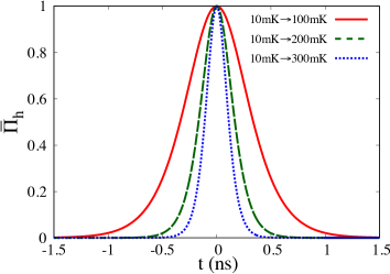
Figure 2: (Color online) Schematic of the function $\bar{\Pi}_{h}(t)$ for different temperatures. The red solid, green dashed and blue dotter curves represent the heating up from $T_{\rm S}=10$mK to $T_{\rm D}=100$mK, $200$mK and $300$mK, respectively.

To achieve such requirement, one need to find a proper $V(t)$ so that the power spectral density of $e^{-i\phi(t)}$ follows $\Pi_{h}(\omega)$, i.e.,

$$\Pi_{h}(\omega) =\Pi_{\rm V}(\omega)= |\frac{1}{\sqrt{t_{0}}}\int^{t_{0}}_{0}dte^{i\omega t}e^{-i\phi(t)}|^{2},$$ (16)

with $\phi(t)$ given below Eq. (8). It should be noted that since $\Pi_{\rm V}(\omega)$ is non-negative according to Eq. (13), equation (16) cannot be satisfied for $T_{\rm D}<T_{\rm S}$, since $\Pi_{h}(\omega)$ can be negative in this case.

Finding $V(t)$ satisfying the requirement Eq. (16) is equivalent to the problem of phase control of pulse shaping, which has been extensively studied in the field of ultrafast optics.Weiner (2011) The basic idea is to attack the problem by working out the Fourier transformation in Eq. (16) within the stationary phase approximation. Here we only outline the procedure, leaving the technical details to the Appendix B.

Within the stationary phase approximation, Eq. (16) can be satisfied by requiring the voltage pulse $V(t)$ follows the relation

$$\frac{t}{t_{0}} = \int^{\frac{e}{\hbar}V(t)}_{-\infty}\frac{d\omega}{2\pi}\Pi_{h}(\omega),$$ (17)

with $t\in[0,t_{0}]$. An analytical solution of Eq. (17) can be obtained by approximating $\Pi_{h}(\omega)$ via the Gaussian ansatz[see Appendix A for details]

$$\Pi_{h}(\omega) \approx \frac{\sqrt{2\pi}}{\sigma_{h}}e^{-\frac{1}{2}(\frac{\omega}{\sigma_{h}})^{2}},$$ (18)

where $\sigma_{h}=\pi k_{\rm B}T_{h}/\sqrt{3}$ with $T_{h}=\sqrt{T^{2}_{\rm D}-T^{2}_{\rm S}}$.

Substituting Eq. (18) into Eq. (17), one has

$$V(t) = \sqrt{2}\sigma_{h}\operatorname{erf}^{-1}(\frac{2t}{t_{0}}).$$ (19)

By further applying the approximation $\operatorname{erf}^{-1}(x)\approx\frac{\sqrt{6}}{\pi}\operatorname{arctanh}(x)$, the above equation reduced to

$$V(t) = 2\frac{\hbar}{e}\sqrt{\frac{\sqrt{3}}{\pi}k_{\rm B}T_{h}}\operatorname{arctanh}(\frac{t-t_{0}}{t_{0}}),$$ (20)

which is just Eq. (1) given in Sec. I.

Note that there are some freedom in the choice of the pulse duration $t_{0}$. In principle, $t_{0}$ should be large enough so that the stationary phase approximation holds. In the realistic calculation, we find that it is adequate to choose $t_{0}$ to be two times larger than the Full width at half maximum (FWHM) of the profile $\bar{\Pi}_{h}(t)$. According to Fig. 2, the typical value of $t_{0}$ is of the order of $1$ ns at sub-kelvin temperatures, corresponding to the frequency of the order of $1$ GHz. One may also worry about the divergence of the function $\operatorname{arctanh}(\tau)$ at the boundary $\tau=\pm 1$ in Eq. (20). This can be fixed by set a limit of the amplitude of $V(t)$, which has minor influence if the overall profile of $V(t)$ does not change too much.

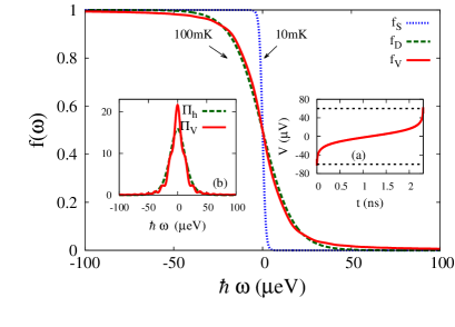
Figure 3: (Color online) The energy distribution of the incoming and outgoing electrons (main panel). The blue dotted curves represents the distribution of the incoming electron $f_{\rm S}$, which is the Fermi distribution at the temperature $T_{\rm S}=10$ mK. The distribution of the outgoing electrons $f_{\rm V}$ are shown with red solid curves. The green dashed curve represent the Fermi distribution at the temperature $T_{\rm D}=100$ mK. The voltage pulse $V(t)$ with duration $t_{0}=2.3$ ns is shown in inset (a), the amplitude of $V(t)$ is limited to $60$ $\mu$V as indicated by the black dotted lines. The integral kernel $\Pi_{\rm V}(\omega)$ corresponding to $V(t)$(red solid curve) is compared to the integral kernel $\Pi_{h}(\omega)$ from Eq. (14)(green dashed curve) in the inset (b).

Despite the approximation we have used in above derivation, the time-averaged energy distribution of the outgoing electron produced by the voltage pulse $V(t)$ can follow the desired Fermi distribution quite well, which we demonstrate in Fig. 3. In the main panel of the figure, the blue dotted curves represents the energy distribution $f_{\rm S}(\omega)$ of the incoming electrons from reservoir A, which is the Fermi distribution at the temperature $T_{\rm S}=10$ mK and chemical potential $\mu=0$. The red solid curve represents the time-averaged distribution $f_{\rm V}(\omega)$ of the outgoing electrons, which is calculated by numerical integrating Eqs. (13) with the voltage pulse $V(t)$[Eq. (20)] of the parameter $T_{h}=99.5$ mK. One can see that it follows the Fermi distribution at the temperature $T_{\rm D}=100$ mK(green dashed curve), which agrees with the analytical expression given in Eq. (20).

The temporal profile of the applied voltage pulse $V(t)$ is shown in the inset (a) of Fig. 3. The pulse duration $t_{0}$ is chosen to be $2.3$ ns, which is just equal to two times of the FWHM of the corresponding $\bar{\Pi}_{h}(t)$[red solid curve in Fig. 2]. The amplitude limit of $V(t)$ is set to $60$ $\mu$V, which has little impact on the overall profile of the pulse. In the inset (b), we also compare the integral kernel $\Pi_{\rm V}(\omega)$[calculated from $V(t)$ via Eqs. (13)] to the integral kernel $\Pi_{h}(\omega)$ given in Eq. (14). One can see that, despite some small ripples, the overall profile of the two kernel agrees with each other, which justifies the approximation we have used in the derivation.

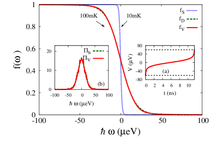
Figure 4: (Color online) The same as Fig. 3, but with the pulse duration $t_{0}=11.5$ ns.

By further increasing the pulse duration $t_{0}$, the ripples in the integral kernel can be suppressed, as can be seen from Fig. 4. Comparing to Fig. 3, we have increase $t_{0}$ to $11.5$ ns, while keeping other parameter fixed. The suppression of the ripples in the integral kernel can be clearly in the inset (b) of Fig. 4. As a consequence, the energy distribution of the outgoing electrons(red solid curve) agrees quite well with the Fermi distribution with $T_{\rm D}=100$ mK(green dashed curve), so that they are almost indistinguishable from each other in the main panel of the figure.

Hence, one can see that, applying the voltage pulse $V(t)$ with the temporal profile given in Eq. (20), the energy distribution of the outgoing electrons can be tuned to follow the Fermi distribution from Eq. (2) quite well. According to Eq. (20), to achieve such tuning for higher temperature $T_{\rm D}$, voltage pulse with larger amplitude is required. In this case, the amplitude limit of the pulse can have more pronounced impact on the result.

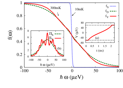
Figure 5: (Color online) The same as Fig. 3, but with the temperature $T_{\rm D}=300$ mK and the corresponding $T_{h}=299.8$ mK.

Such impact is demonstrated in Fig. 5. All the parameters are chosen the same as Fig. 3, except the temperature $T_{\rm D}$, which is increased to $300$ mK in this case. From the inset (a), one can see that the pulse profile is modified due to the amplitude limit of the pulse, leading to small platforms close to the edges. As a consequence, these platforms induces ripples in the corresponding integral kernel, which is shown in the inset (b). Such ripples can also be identified in the energy distribution of the outgoing electron, which is shown as red solid curve in the main panel of the figure.

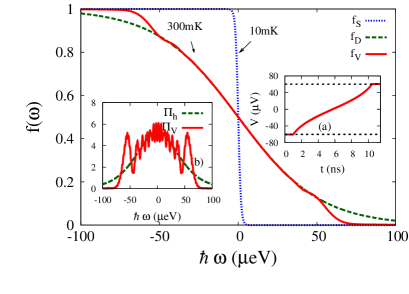
Figure 6: (Color online) The same as Fig. 5, but with the pulse duration $t_{0}=11.5$ ns.

Note that in the case where the profile of the pulse has been changed due to the amplitude limitation, the induced ripples cannot be suppressed by increasing the pulse duration $t_{0}$, which we demonstrate in Fig. 6. In this case, all the parameters are chosen the same as Fig. 5, except the pulse duration $t_{0}$, which is increased to $11.5$ ns. One can still identify large ripples in the integral kernel[inset (b)]. The impact of these ripples can lead to pronounced distortion of the energy distribution of outgoing electrons far from the Fermi level, which can be seen in the main panel of Fig. 6.

It should be noted that in the realistic situation, the voltage pulse can also lead to Joule heating.Kumar et al. (1996) To make the manipulation observable, the amplitude of the voltage pulse should be kept low enough so that the Joule heating is not significant. It has been reported that in typical quantum point contacts, voltage pulses with the root mean square amplitude $60$ $\mu$V can heat up the electrons to about $50$ mK,Dubois et al. (2013) which is smaller then the effect we shown here. So we expect that such manipulation can be experimentally detected in a realistic system.

IV Shot noise thermometer

Experimentally, the time-averaged energy distribution of the outgoing electrons can be detected via an adjustable energy filter, which can be realized by using a quantum dot fabricated at a certain distance from the voltage source.Altimiras et al. (2010); Kovrizhin and Chalker (2011) However, as the profile of the energy distribution can be changed during the propagation due to various energy relaxation mechanisms, such as the coupling to electrons on counter-propagating edge channels,Le Sueur et al. (2010); Kovrizhin and Chalker (2012); Venkatachalam et al. (2012); Prokudina et al. (2014) it is more favorable to detect the distribution in situ at the voltage pulse source. This can be done by using the shot noise thermometry technique,Spietz et al. (2003) which we will discuss in this section.

In the standard shot noise thermometry technique, the electron temperature is extracted from the DC-bias-voltage dependence of the current noise across a tunneling barrier.Spietz et al. (2003) This can be implemented in the voltage pulse electron source by introducing a static potential in the short interval at the center of the wire, which is illustrated in Fig. 7. Note that the static potential is assumed to be rapidly-varying comparing to the Fermi wavelength $1/k_{\rm F}$, which can lead to backscattering between left- and right-going electrons in the system.

Following the scattering formalism, the scattering between the left- and right-going electrons can be described by the time-dependent scattering matrixBlanter and Büttiker (2000); Ivanov et al. (1997)

$$\left(\begin{tabular}[]{c}$\hat{b}_{1}(t)$\\ $\hat{a}_{2}(t)$\\ \end{tabular}\right)=S(t)\left(\begin{tabular}[]{c}$\hat{a}_{1}(t)$\\ $\hat{b}_{2}(t)$\\ \end{tabular}\right),$$ (25)

$$S(t)=\left(\begin{tabular}[]{cc}$\sqrt{D_{0}}e^{-i\phi(t)}$&$-i\sqrt{1-D_{0}}$\\ $-i\sqrt{1-D_{0}}$&$\sqrt{D_{0}}e^{i\phi(t)}$\\ \end{tabular}\right),$$ (28)

with $D_{0}$ being the time-independent transmission coefficient due to the static potential. The Fermi operator $\hat{a}_{1(2)}$ and $\hat{b}_{2(1)}$ represent the incoming(outgoing) electrons modes from(towards) the reservoir A and B, respectively. The phase factor $\phi(t)$ is given below Eq. (8). For simplicity, we assume both the reservoir A and B are kept at the same temperature $T_{\rm S}$ and chemical potential $\mu$.

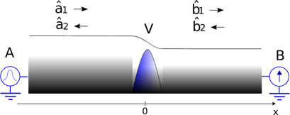
Figure 7: (Color online) Schematic of the voltage pulse source with a static potential barrier, which mixes the left-going (represented by $\hat{a}_{1}$ and $\hat{b}_{1}$) and right-going (represented by $\hat{a}_{2}$ and $\hat{b}_{2}$) electrons.

Consider the time-averaged current noise detected at the reservoir B, it can be given as

$$S_{\rm B} =\frac{1}{t_{0}} \int^{t_{0}}_{0}dt\int^{t_{0}}_{0}dt^{\prime}\Big{[}\left<\hat{j}_{\rm B}(t)\hat{j}_{\rm B}(t^{\prime})\right>$$ (29)

$$\hskip 42.67912pt\mbox{}-\left<\hat{j}_{\rm B}(t)\right>\left<\hat{j}_{\rm B}(t^{\prime})\right>\Big{]},$$

where the current operator $\hat{j}_{\rm B}(t)$ has the form

$$\hat{j}_{\rm B}(t) = \hat{b}^{\dagger}_{1}(t)\hat{b}_{1}(t)-\hat{b}^{\dagger}_{2}(t)\hat{b}_{2}(t).$$ (30)

By using the time-dependent scattering matrix Eq. (28), the current noise can be written as

$$S_{B} = S_{e}+S_{n},$$ (31)

with $S_{e}$ and $S_{n}$ being the equilibrium and non-equilibrium contribution, respectively. The equilibrium term

$$S_{e} = \frac{e^{2}}{2\pi\hbar}D^{2}_{0}\int\frac{d\omega}{2\pi}\Big{\{}\big{[}1-f_{\rm S}(\Omega)\big{]}f_{\rm S}(\omega)$$ (32)

$$\hskip 42.67912pt\mbox{}+f_{\rm S}(\omega)\big{[}1-f_{\rm S}(\omega)\big{]}\Big{\}},$$

is just the Nyquist-Johnson noise which is independent on the applied DC bias voltage. The non-equilibrium term, i.e., the shot noise term, can be written as

$$S_{n} = \frac{e^{2}}{2\pi\hbar}D_{0}(1-D_{0})\int\frac{d\omega}{2\pi}\Big{\{}\big{[}1-f_{\rm S}(\omega)\big{]}f_{\rm V}(\omega)$$ (33)

$$\hskip 42.67912pt\mbox{}+f_{\rm V}(\omega)\big{[}1-f_{\rm S}(\omega)\big{]}\Big{\}},$$

with $f_{\rm V}(\omega)$ given in Eqs. (13).

One can see immediately that, if $f_{\rm V}(\omega)$ is tuned to the Fermi distribution $f_{\rm D}(\omega)$ given in Eq. (2), then Eq. (33) should be equal to

$$\bar{S}_{n} = \frac{e^{2}}{2\pi\hbar}D_{0}(1-D_{0})\int\frac{d\omega}{2\pi}\Big{\{}\big{[}1-f_{\rm S}(\omega)\big{]}f_{\rm D}(\omega)$$ (34)

$$\hskip 42.67912pt\mbox{}+f_{\rm S}(\omega)\big{[}1-f_{\rm D}(\omega)\big{]}\Big{\}},$$

which is just the shot noise between two reservoirs with different temperature $T_{\rm S}$ and $T_{\rm D}$. Hence, to check if the manipulation of the energy distribution is properly achieved, one just compare the DC bias dependence $S_{n}$ from Eq. (33) to the predicted one $\bar{S}_{n}$ from Eq. (34).

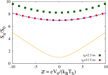
Figure 8: (Color online) Normalized shot noise $S_{n}/S_{0}$ as a function of normalized DC bias voltage $x=eV_{0}/(k_{\rm B}T_{\rm S})$, with $S_{0}=e^{2}D_{0}(1-D_{0})k_{\rm B}T_{\rm S}/(2\pi^{2}\hbar)$ being the zero-bias noise. The temperature $T_{\rm S}$ of the reservoirs A and B is chosen to be $T_{\rm S}=10$ mK. The green squares and red dots are shot noise with voltage pulse duration $t_{0}=2.3$ ns and $11.5$ ns, corresponding to the case in Fig. 3 and Fig. 4, respectively. The blue dotted curve represents the normalized shot noise between two reservoirs at temperature $T_{\rm S}$ and $T_{\rm D}$. The orange dashed curve represents the universal function $x/\tanh(x/2)$.

As an example, we perform such comparison for the case with $T_{\rm S}=10$ mK and $T_{\rm D}=100$ mK in Fig. 8. The shot noise is normalized to the zero-bias noise $S_{0}=e^{2}D_{0}(1-D_{0})k_{\rm B}T_{\rm S}/(2\pi^{2}\hbar)$, which is plotted as a function of the normalized voltage $x=eV_{0}/(k_{\rm B}T_{\rm S})$. The predicted $\bar{S}_{n}$ from Eq. (34) is plotted as blue dotted curve. The green squares represent the shot noise obtained by applying the voltage pulse $V(t)$ with $t_{0}=2.3$ ns, while the red dots correspond to the case with $t_{0}=11.5$ ns. The corresponding energy distribution of the outgoing electrons can be found in Fig. 3[$t_{0}=2.3$ ns] and Fig. 4[$t_{0}=11.5$ ns], respectively. One can see that, by increasing $t_{0}$, the profile of the distribution of outgoing electrons approaches the Fermi distribution $f_{\rm D}(\omega)$[Fig. 3 and Fig. 4] , while the shot noise approaches the predicted shot noise $\bar{S}_{n}$, indicating that the shot noise can be used as a hallmark of the profile of the energy distribution of the outgoing electrons. Note that without the voltage pulse $V(t)$, the normalized shot noise follows the well-known universal function $x/\tanh(x/2)$, which is shown as orange dashed curves in the figure.

V SUMMARY

In summary, we have propose a scheme to manipulate the electron-hole excitation in the voltage pulse electron source. By using stationary phase approximation, we derive a simple analytical expression of the voltage pulse $V(t)$ [Eq. (1)], which can tuned the electron-hole excitation so that the energy distribution of the emitted electrons from the electron source follows a desired Fermi distribution with higher temperature. Such distribution can be established without introducing additional energy relaxation mechanism. We also show that such distribution can be detected in situ at the voltage pulse electron source via shot noise thermometry technique, making it helpful in the study of thermal transport and decoherence in mesoscopic system.

Appendix A Derivation of Eq. (14), (15) and (18)

In this appendix, we derive the integral kernel $\Pi_{h}(\omega)$ given in Eqs. (14) and (15). It satisfies the condition

$$f_{\rm D}(\omega) = \int\frac{d\omega^{\prime}}{2\pi}f_{\rm S}(\omega^{\prime})\Pi_{\rm h}(\omega-\omega^{\prime}),$$ (35)

with $f_{\rm D}(\omega)$ and $f_{\rm S}(\omega)$ being the Fermi distribution given in Eq. (2) and Eq. (11), respectively.

This equation can be solved via Fourier transformation. Taking the derivative with respect to $\omega$ on both side of Eq. (35), one has

$$\frac{\beta_{\rm D}}{4}\frac{1}{\cosh^{2}[\frac{\beta_{\rm D}(\mu-\hbar\omega)}{2}]} = \int\frac{d\omega^{\prime}}{2\pi}\Pi_{\rm h}(\omega-\omega^{\prime})$$ (36)

$$\mbox{}\times\frac{\beta_{\rm S}}{4}\frac{1}{\cosh^{2}[\frac{\beta_{\rm S}(\mu-\hbar\omega)}{2}]},$$

with $\beta_{\rm S(D)}=1/[k_{\rm B}T_{\rm S(D)}]$.

Performing the Fourier transformation on both side of Eq. (36) and using the identity

$$\int dx\frac{e^{ixy}}{\cosh^{2}(x)} = \frac{\pi y}{\sinh(\frac{\pi}{2}y)},$$ (37)

one obtains

$$\frac{t}{2\beta_{\rm D}\sinh(\frac{\pi}{\beta_{\rm D}}t)} = \frac{t}{2\beta_{\rm S}\sinh(\frac{\pi}{\beta_{\rm S}}t)}\bar{\Pi}_{h}(t),$$ (38)

with

$$\Pi_{h}(\omega) = \int dte^{i\omega t}\bar{\Pi}_{h}(t),$$ (39)

which gives $\Pi_{h}(\omega)$ given in Eq. (14) and (15).

One can also apply a Gaussian approximation for the derivative of the distribution function. In this case, one assume

$$f_{\rm S(D)}(E) = 1-\int^{E}_{0}dE^{\prime}g_{\rm S(D)}(E^{\prime}),$$ (40)

with

$$g_{\rm S(D)}(E) = \frac{1}{\sqrt{2\pi}\sigma_{\rm S(D)}}e^{-\frac{1}{2}(\frac{E-\mu}{\sigma_{\rm S(D)}})^{2}},$$ (41)

where the width $\sigma_{\rm S(D)}$ is chosen so that the average energy of the system satisfies

$$\int^{+\infty}_{0}f_{\rm S(D)}(E^{\prime})(E^{\prime}-\mu)dE^{\prime} = \frac{(\pi k_{\rm B}T_{\rm S(D)})^{2}}{6},$$ (42)

which gives $\sigma_{\rm S(D)}=\pi k_{\rm B}T_{\rm S(D)}/\sqrt{3}$. By combining the Gaussian approximation with Eq. (35), the integral kernel can be approximated via

$$\Pi_{h}(\omega) \approx \frac{\sqrt{2\pi}}{\sigma_{h}}e^{-\frac{1}{2}(\frac{\omega}{\sigma_{h}})^{2}},$$ (43)

with $\sigma_{h}=\pi k_{\rm B}T_{h}/\sqrt{3}$ with $T_{h}=\sqrt{T^{2}_{\rm D}-T^{2}_{\rm S}}$, which is just Eq. (18).

Appendix B Phase control of pulse shaping

In this appendix, we introduce the phase control of the pulse shaping following Ref. Cook, 2012, which we have used in the derivation of Eq. (17) from Eq. (16).

The problem of phase control of pulse shaping is to find a signal

$$s(t) = a(t)\exp[i\theta(t)],$$ (44)

whose power spectral density follows a given function $U(\omega)$, i.e.,

$$U(\omega)\exp[i\Phi(\omega)] = \int^{+\infty}_{-\infty}dta(t)\exp[i\theta(t)-i\omega t],$$ (45)

with $\Phi(\omega)$ being an arbitrary function. Here $a(t)$, $\theta(t)$, $\Phi(\omega)$ and $U(\omega)$ are all real.

To attack this problem, one first evaluate the Fourier transformation Eq. (45) by using the stationary phase approximation. For a given $\omega$, this can be done by performing the Taylor expansion of the phase factor around $t=T_{\omega}$ as

$$\omega t-\theta(t) = [\omega T_{\omega}-\theta(T_{\omega})]+[\omega-\theta^{\prime}(T_{\omega})](t-T_{\omega})$$ (46)

$$\mbox{}+\theta^{\prime\prime}(T_{\omega})(t-T_{\omega})^{2}+...,$$

where $T_{\omega}$ is obtained by using the stationary phase condition

$$\omega = \theta^{\prime}(T_{\omega}).$$ (47)

Here $\theta^{\prime}(t)$ and $\theta^{\prime\prime}(t)$ represents the first- and second-order derivative of the function $\theta(t)$ over time $t$, respectively.

Substituting Eqs. (46) and (47) into Eq. (45), one obtains

$$U(\omega)\exp[i\Phi(\omega)] \approx \sqrt{\frac{2\pi}{\theta^{\prime\prime}({T_{\omega}})}}a(T_{\omega})$$ (48)

$$\mbox{}\times\exp[-i\omega T_{\omega}+i\theta(T_{\omega})+\frac{\pi}{4}],$$

from which one has

$$a^{2}(T_{\omega}) = U^{2}(\omega)\frac{\theta^{\prime\prime}(T_{\omega})}{2\pi}.$$ (49)

By combining Eq. (49) with the stationary phase condition Eq. (47), one can obtain a differential equation, from which $\theta(t)$ can be solved if the function $a(t)$ and $U(\omega)$ are known. To make this clear, let $x=\omega$ and $y=T_{\omega}$, Eqs. (47) and (49) have the form

$$x = \frac{d\theta(y)}{dy},$$ (50)

$$a^{2}(y) = \frac{U^{2}(x)}{2\pi}\frac{d^{2}\theta(y)}{d^{2}y}.$$ (51)

Substituting Eq. (50) into Eq. (51), one can eliminate $\theta(y)$, which gives the differential equation

$$a^{2}(y)dy = \frac{U^{2}(x)}{2\pi}dx,$$ (52)

from which the function $y(x)$[or equivalent, the function $x(y)$] can be solved. The phase $\theta(y)$ can then be obtained from Eq. (50).

To applying the above procedure to solve Eq. (16), one choose

$$a(y) = \left\{\begin{tabular}[]{cc}$1/\sqrt{t_{0}}$&, $y\in[0,t_{0}]$\\ $0$&, otherwise\\ \end{tabular}\right.,$$ (55)

and $U^{2}(x)=\Pi_{h}(x)$. Integrating both side of Eq. (51), one has

$$\int^{y}_{-\infty}a^{2}(y^{\prime})dy^{\prime} = \int^{x}_{-\infty}\frac{dx^{\prime}}{2\pi}\Pi_{h}(x).$$ (56)

This equation can be reduced to Eq. (17) for $y\in[0,t_{0}]$ by performing the substitution $y\rightarrow t$ and

$$x\rightarrow\frac{e}{\hbar}V(t)=\frac{d\phi(t)}{dt}.$$ (57)

References

- Oliver et al. (1999) W. D. Oliver, J. Kim, R. C. Liu, and Y. Yamamoto, Science 284, 299 (1999).
- Henny et al. (1999) M. Henny, S. Oberholzer, C. Strunk, T. Heinzel, K. Ensslin, M. Holland, and C. Schönenberger, Science 284, 296 (1999).
- Bertoni et al. (2000) A. Bertoni, P. Bordone, R. Brunetti, C. Jacoboni, and S. Reggiani, Phys. Rev. Lett. 84, 5912 (2000).
- Ionicioiu et al. (2001) R. Ionicioiu, G. Amaratunga, and F. Udrea, Int. J. Mod. Phys. B 15, 125 (2001).
- Ji et al. (2003) Y. Ji, Y. Chung, D. Sprinzak, M. Heiblum, D. Mahalu, and H. Shtrikman, Nature 422, 415 (2003).
- Bocquillon et al. (2014) E. Bocquillon, V. Freulon, F. D. Parmentier, J.-M. Berroir, B. Plaçais, C. Wahl, J. Rech, T. Jonckheere, T. Martin, C. Grenier, D. Ferraro, P. Degiovanni, and G. Fève, Ann. Phys. 526, 1 (2014).
- Glattli and Roulleau (2017) D. C. Glattli and P. S. Roulleau, Phys. Stat. Sol. (b) 254 (2017).
- Vanević et al. (2016) M. Vanević, J. Gabelli, W. Belzig, and B. Reulet, Phys. Rev. B 93, 041416 (2016).
- Lee and Levitov (1993) H. Lee and L. Levitov, cond-mat/9312013 (1993).
- Lee and Levitov (1995) H. Lee and L. Levitov, cond-mat/9507011 (1995).
- Keeling et al. (2006) J. Keeling, I. Klich, and L. Levitov, Phys. Rev. Lett. 97, 116403 (2006).
- Dubois et al. (2013) J. Dubois, T. Jullien, F. Portier, P. Roche, A. Cavanna, Y. Jin, W. Wegscheider, P. Roulleau, and D. Glattli, Nature 502, 659 (2013).
- Jullien et al. (2014) T. Jullien, P. Roulleau, B. Roche, A. Cavanna, Y. Jin, and D. Glattli, Nature 514, 603 (2014).
- Gabelli et al. (2017) J. Gabelli, K. Thibault, G. Gasse, C. Lupien, and B. Reulet, Phys. Stat. Sol. (b) 254 (2017).
- Moskalets (2016) M. Moskalets, Phys. Rev. Lett. 117, 046801 (2016).
- Schwab et al. (2000) K. Schwab, E. A. Henriksen, J. M. Worlock, and M. L. Roukes, Nature 404, 974 (2000).
- Chiatti et al. (2006) O. Chiatti, J. T. Nicholls, Y. Y. Proskuryakov, N. Lumpkin, I. Farrer, and D. A. Ritchie, Phys. Rev. Lett. 97, 056601 (2006).
- Chen et al. (2009) Y.-F. Chen, T. Dirks, G. Al-Zoubi, N. O. Birge, and N. Mason, Phys. Rev. Lett. 102, 036804 (2009).
- Granger et al. (2009) G. Granger, J. Eisenstein, and J. Reno, Phys. Rev. Lett. 102, 086803 (2009).
- Altimiras et al. (2010) C. Altimiras, H. Le Sueur, U. Gennser, A. Cavanna, D. Mailly, and F. Pierre, Nature Physics 6, 34 (2010).
- Le Sueur et al. (2010) H. Le Sueur, C. Altimiras, U. Gennser, A. Cavanna, D. Mailly, and F. Pierre, Phys. Rev. Lett. 105, 056803 (2010).
- Venkatachalam et al. (2012) V. Venkatachalam, S. Hart, L. Pfeiffer, K. West, and A. Yacoby, Nature Physics 8 (2012).
- Jezouin et al. (2013) S. Jezouin, F. D. Parmentier, A. Anthore, U. Gennser, A. Cavanna, Y. Jin, and F. Pierre, Science 342, 601 (2013).
- Spietz et al. (2003) L. Spietz, K. Lehnert, I. Siddiqi, and R. Schoelkopf, Science 300, 1929 (2003).
- Blanter and Büttiker (2000) Y. M. Blanter and M. Büttiker, Physics Reports 336, 1 (2000).
- Ivanov et al. (1997) D. Ivanov, H. Lee, and L. Levitov, Phys. Rev. B 56, 6839 (1997).
- Keeling et al. (2008) J. Keeling, A. Shytov, and L. Levitov, Phys. Rev. Lett. 101, 196404 (2008).
- Grenier et al. (2011) C. Grenier, R. Hervé, E. Bocquillon, F. D. Parmentier, B. Plaçais, J.-M. Berroir, G. Fève, and P. Degiovanni, New Journal of Physics 13, 093007 (2011).
- Haack et al. (2011) G. Haack, M. Moskalets, J. Splettstoesser, and M. Büttiker, Phys. Rev. B 84, 081303 (2011).
- Haack et al. (2013) G. Haack, M. Moskalets, and M. Büttiker, Phys. Rev. B 87, 201302 (2013).
- Kovrizhin and Chalker (2011) D. Kovrizhin and J. Chalker, Phys. Rev. B 84, 085105 (2011).
- Kovrizhin and Chalker (2012) D. Kovrizhin and J. Chalker, Phys. Rev. Lett. 109, 106403 (2012).
- Moskalets (2014) M. Moskalets, Phys. Rev. B 89, 045402 (2014).
- Weiner (2011) A. M. Weiner, Optics Communications 284, 3669 (2011).
- Kumar et al. (1996) A. Kumar, L. Saminadayar, D. Glattli, Y. Jin, and B. Etienne, Phys. Rev. Lett. 76, 2778 (1996).
- Prokudina et al. (2014) M. Prokudina, S. Ludwig, V. Pellegrini, L. Sorba, G. Biasiol, and V. Khrapai, Phys. Rev. Lett. 112, 216402 (2014).
- Cook (2012) C. Cook, Radar signals: An introduction to theory and application (Elsevier, 2012).