Quantum Monte Carlo study of static potential in graphene

Abstract

In this paper the interaction potential between static charges in suspended graphene is studied within the quantum Monte Carlo approach. We calculated the dielectric permittivity of suspended graphene for the set of temperatures and extrapolated our results to zero temperature. The dielectric permittivity at zero temperature has the following properties. At zero distance $\epsilon=2.24\pm 0.02$. Then it rises and at a large distance the dielectric permittivity reaches the plateau $\epsilon\simeq 4.20\pm 0.66$. The results obtained in this paper allow to draw a conclusion that full account of many-body effects in the dielectric permittivity of suspended graphene gives $\epsilon$ very close to the one-loop results. Contrary to the one-loop result, the two-loop prediction for the dielectric permittivity deviates from our result. So, one can expect large higher order corrections to the two-loop prediction for the dielectric permittivity of suspended graphene.

I Introduction

Graphene, two dimensional crystal composed of carbon atoms packed in a honeycomb lattice Novoselov:04:1 ; Geim:07:1 , attracts considerable interest due to its electronic properties. There are two Fermi points in the electronic spectrum of graphene. In the vicinity of each point the fermion excitations are similar to the massless Dirac fermions living in two dimensions wallace ; semenoff ; Novoselov:05:1 ; zhang . Relativistic nature of fermion excitations in graphene leads to numerous quantum relativistic phenomena such as Klein tunneling, minimal conductivity through evanescent waves, relativistic collapse at a supercritical charge and etc. Guinea ; Kotov:2 ; Katsnelson .

The Fermi velocity in graphene is much smaller than the speed of light ($v_{F}\sim c/300$), resulting in negligible retardation effects and magnetic interaction between quasiparticles. Thus the interaction in graphene can be approximated by the instantaneous Coulomb potential with the large effective coupling constant $\alpha_{eff}=\alpha\cdot c/v_{F}\sim 300/137\sim 2.2$.

It is reasonable to assume that the observables in graphene theory are considerably renormalized due to strong interaction as compared to the non-interacting theory. For instance, the leading perturbative renormalization of the Fermi velocity with the logarithmic accuracy Gonzalez:1993uz ; Mishchenko ; Herbut ; Fritz ; Fernando leads to the increase of $v_{F}$ as large as $\sim 100\%$ for suspended graphene. One can expect that higher order renormalization leads to further considerable change of the bare value of the Fermi velocity. However, existing experimental measurements of the Fermi velocity Elias ; PNAS are in a good agreement with the first-order perturbation theory improved by the one-loop expression for the dielectric permittivity of graphene. Recently it was shown that the next-to-leading order corrections in the random phase approximation (RPA) are small relative to the leading-order RPA results dassarma . Nevertheless it is not clear what happens to the perturbative corrections after the next-to-leading order.

Another important observable in graphene is the interaction potential between static charges. The renormalization of the static potential can be parameterized by the dielectric permittivity depending on the distance between static charges $\epsilon(r)$. One-loop expression for $\epsilon(r)$ was calculated in Astrakhantsev:2015cla . At small distances $\epsilon(r)\sim 2$. Then the dielectric permittivity grows with the distance and at large distances $r\gg a$ it reaches well known one-loop expression Katsnelson ; Kotov:2

$$\epsilon=1+\frac{\pi}{2}\alpha_{eff}.$$ (1)

For $\alpha_{eff}=2.2$ this formula gives $\epsilon=4.4$. So, one sees that the one-loop correction is very large. Two-loop correction to $\epsilon$ was calculated in fogler and can be written as

$$\epsilon=1+\frac{\pi}{2}\alpha_{eff}+0.778\alpha_{eff}^{2}.$$ (2)

If one takes $\alpha_{eff}=2.2$ the dielectric permittivity is $\epsilon=8.2$. If one accounts one-loop renormalization of $\alpha_{eff}$ (see below), $\epsilon\simeq 2.5$. So, it is clear that the next-to-leading order corrections considerably modify the one-loop result. One can also expect that higher order corrections are also significant.

In this paper we are going to study the interaction potential between static charges in suspended graphene within quantum Monte Carlo simulations (see Ulybyshev:2013swa for details). The first Monte Carlo study of the static interaction potential based on the low energy effective theory of graphene was done in paper Braguta:2013rna . In this paper we are going to use the approach which is based on the tight-binding Hamiltonian without the expansion near the Fermi points. This approach allows to avoid ambiguity due to regularization procedure. In addition, the interactions between quasiparticles are parameterized by the realistic phenomenological potential obtained in Wehling that significantly deviates from the Coulomb potential at small distances. However, the main advantage of the Monte-Carlo approach is that it fully accounts interactions between quasiparticles basing on the first principles.

This paper is organized as follows. In the next section we briefly describe the method of lattice Monte Carlo simulation of graphene. Section III is devoted to the discussion of how the potential of static charges can be calculated within Monte Carlo simulations. The results of the calculation are presented in Section IV. In the last section we summarize our results.

II Brief description of the model

In the calculation we use the tight-binding model of graphene. The Hamiltonian consists of the tight-binding term and the interaction part describing the full electrostatic interaction between quasiparticles:

$$\hat{H}=-\kappa\sum\limits_{<x,y>}\left(\hat{a}^{{\dagger}}_{y,\uparrow}\hat{a}_{x,\uparrow}+\hat{a}^{{\dagger}}_{y,\downarrow}\hat{a}_{x,\downarrow}+h.c.\right)$$

$$+\sum\limits_{x=\{1,\xi\}}m(\hat{a}^{{\dagger}}_{x,\uparrow}\hat{a}_{x,\uparrow}-\hat{a}^{{\dagger}}_{x,\downarrow}\hat{a}_{x,\downarrow})$$

$$-\sum\limits_{x=\{2,\xi\}}m(\hat{a}^{{\dagger}}_{x,\uparrow}\hat{a}_{x,\uparrow}-\hat{a}^{{\dagger}}_{x,\downarrow}\hat{a}_{x,\downarrow})$$

$$+{1\over 2}\,\sum\limits_{x,y}V_{xy}\hat{q}_{x}\hat{q}_{y},$$ (3)

where $\kappa=2.7\,{\rm eV}$ is the hopping between nearest-neighbors, $\hat{a}^{{\dagger}}_{x,\uparrow}$, $\hat{a}_{x,\uparrow}$ and $\hat{a}^{{\dagger}}_{x,\downarrow}$, $\hat{a}_{x,\downarrow}$ are creation/annihilation operators for spin-up and spin-down electrons at $\pi$-orbitals. Spatial index $x=\{s,\xi\}$ consists of sublattice index $s=1,2$ and two-dimensional coordinate $\xi=\{\xi_{1},\xi_{2}\}$ of the unit cell in rhombic lattice. Periodic boundary conditions are imposed in both spatial directions in the manner of Ulybyshev:2013swa . The mass term has different sign at two sublattices. According to the simulation algorithm, one should introduce the mass in order to eliminate zero modes from the fermionic determinant. The calculation is carried out at few various masses and the final results are obtained through the chiral extrapolation $m\to 0$.

The matrix $V_{xy}$ is the bare electrostatic interaction potential between sites with coordinates $x$ and $y$ and $\hat{q}_{x}=\hat{a}^{{\dagger}}_{x,\uparrow}\hat{a}_{x,\uparrow}+\hat{a}^{{\dagger}}_{x,\downarrow}\hat{a}_{x,\downarrow}-1$ is the electric charge operator at lattice site $x$. The potential $V_{xy}$ represents the screened Coulomb interaction. At small distances $r/a\leqslant 2$ we employ phenomenological potentials $V_{00},\,V_{01},\,V_{02},\,V_{03}$ calculated in Wehling , while at distances $r/a\geqslant 2$ we use the Coulomb-like potential

$$V(r)=\frac{A}{r/a+C},$$ (4)

where $A=\alpha\cdot\hbar c/a=10.14\,$eV, $C=0.82$. The parameter $C$ is chosen so that $V(2a)=V_{03}$. This choice ensures smooth interpolation between regions of the phenomenological potential and the Coulomb-like potential.

All calculations were performed using the Hybrid Monte-Carlo algorithm. Details of the algorithm are described in Ulybyshev:2013swa . The method is based on the Suzuki-Trotter decomposition. Partition function $\exp(-\beta\hat{H})$ is represented in the form of a functional integral in Euclidean time. Inverse temperature is equal to the number of time slices multiplied by the step in Euclidean time: $\delta\tau L_{t}=\beta=1/T$. Since the algorithm requires fermionic fields to be integrated out, we eliminate all the four-fermionic terms in the full Hamiltonian using the Hubbard-Stratonovich transformation. The final form of the partition function can be written as:

$${\rm Tr}\,e^{-\beta\hat{H}}\cong\int\mathcal{D}\varphi_{x,n}e^{-S\left[\varphi_{x,n}\right]}|\det{M\left[\varphi_{x,n}\right]}|^{2}\,,$$ (5)

where $\varphi_{x,n}$ is the Hubbard-Stratonovich field for timeslice $n$ and spatial coordinate $x$. Particular form of the fermionic operator $M$ is described in Ulybyshev:2013swa . The absence of the sign problem (appearance of the squared modulus of the determinant) is guaranteed by the particle-hole symmetry in graphene at neutrality point. Action for the Hubbard field $S\left[\varphi_{x,n}\right]$ is also a positively defined quadratic form for all choices of the electron-electron interaction used in our paper. Thus we can generate configurations of $\varphi_{x,n}$ by the Monte-Carlo method using the weight (5) and calculate physical quantities as averages over generated configurations.

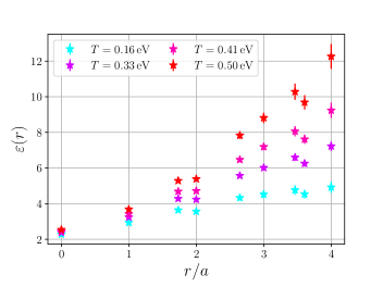
Figure 1: The dielectric permittivity of graphene $\epsilon(r,T)$ as a function of distance $r/a$ for $T=0.167,\,0.333,\,0.417,\,0.5\,$eV.

III Details of the calculation

To calculate the potential of the static charges in graphene one introduces the Polyakov loop of the Hubbard-Stratonovich field. The Polyakov loop is defined as a product of the factors $\exp{(iQ\delta\tau\varphi_{\vec{x},t})}$ over all slices in Eucledean time $t$ and with fixed spatial coordinate $\vec{x}$

$$L_{Q}(\vec{x})=\prod_{t=0}^{L_{t}-1}\text{exp}(-iQ\Delta\tau\varphi_{\vec{x},t}).$$ (6)

Physically the introduction of the operator $\displaystyle L_{Q}(\vec{x})$ implies the calculation of the partition function of graphene with the static charge $Q$

$$\left\langle L_{Q}\right\rangle=\text{exp}(-F_{Q}/T)\,,$$ (7)

where $F_{Q}$ is the free energy of the static charge $Q$ in graphene.

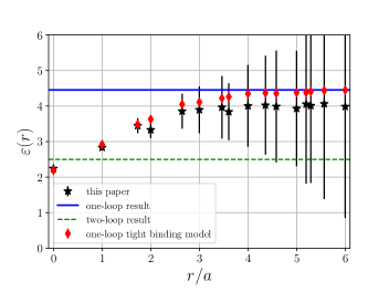
Figure 2: The dielectric permittivity of suspended graphene $\epsilon(r)$ as a function of distance $r/a$ at zero temperature. The results obtained in this paper are represented by black stars. The blue line and green dashed line correspond to the one-loop result (1) and the two-loops result (2) correspondingly. The red diamond points correspond to the one-loop calculation of the $\epsilon(r)$ based on the tight binding model (II) carried out in Astrakhantsev:2015cla .

Similarly the correlation function of the Polyakov loops $\langle L_{Q}(0)L_{Q}^{*}(\vec{r})\rangle$ is determined by the free energy of static charges $Q$ and $-Q$ separated by the distance $\vec{r}$. The free energy of this system is determined by the potential of the static charges in graphene $V_{QQ}(\vec{r})$. Thus we have

$$\left\langle L_{Q}(0)L_{Q}^{*}(\vec{r})\right\rangle\sim\text{exp}(-V_{QQ}(\vec{r})/T)\,.$$ (8)

In order to obtain interaction potential we use the following relation

$$V_{QQ}(\vec{r})=-\frac{T}{Q^{2}}(\text{ln}\left\langle L_{Q}(0)L_{Q}^{*}(\vec{r})\right\rangle-2\text{ln}\left\langle L_{Q}\right\rangle)\,.$$ (9)

In the simulations we considered $Q=0.1$ which significantly improves signal-to-noise ratio both for the correlator and for the Polyakov loop. This value of $Q$ was taken from Braguta:2013rna .

Monte Carlo simulation of graphene was carried out on the lattices with spatial extension $L_{x}=L_{y}=30$. The lattice spacing in temporal direction is $\delta\tau=0.1\,$eV^-1. The temporal sizes of the lattices under study are $L_{t}=60,\,50,\,36,\,34,\,30,\,26,\,24,\,22,\,20$ which correspond to the temperatures $T=0.167,\,0.2,\,0.278,\,0.294,\,0.333,\,0.385,\,0.417,\,0.455,\,0.5\,$eV. For the lattices $30^{2}\times 36\ldots 20$ we conducted the calculations at the following values of the fermion mass $m=0.03,\,0.05,\,0.07,\,0.1\,$eV. For the two lowest temperatures on the lattices $30^{2}\times 60$ and $30^{2}\times 50$ the fermion masses were $0.01,\,0.02,\,0.03,\,0.04\,$eV. For these values of the fermion masses we simulate relativistic fermions. To obtain the results for the massless fermions we fit our data for all temperatures and distances under study by the function $V_{QQ}(r)=V_{0}(r)+V_{1}(r)m^{2}$. For all temperatures and distances the data is well described by this fit ($\chi^{2}\leq 1$). The function $V_{0}(r)$ gives the potential in the massless limit. Below we present the results obtained in the limit of massless fermions $m\to 0$.

$r/a$	$\varepsilon(r)$	$\varepsilon_{\mbox{1 loop}}(r)$
$0.00$	$2.24\pm 0.02$	$2.19$
$1.00$	$2.83\pm 0.08$	$2.92$
$1.73$	$3.45\pm 0.21$	$3.49$
$2.00$	$3.33\pm 0.23$	$3.63$
$2.65$	$3.86\pm 0.49$	$4.05$
$3.00$	$3.89\pm 0.66$	$4.11$
$3.46$	$3.97\pm 0.88$	$4.22$
$3.61$	$3.84\pm 0.80$	$4.26$
$4.00$	$4.01\pm 1.15$	$4.35$

Table 1: The dielectric permittivity of suspended graphene $\epsilon(r)$ as a function of distance $r/a$ at zero temperature. The first column is the distance in graphene lattice units. The second column is the $\epsilon(r)$ calculated in this paper. The third column contains the $\epsilon(r)$ calculated at the one-loop level within the tight binding model (II).

IV Results of the calculation

In Fig. 1 we present the results of the calculation of the dielectric permittivity of graphene $\epsilon(r)$ which is the ratio of the bare potential (4) to the one measured on the lattice (9). The dielectric permittivity is presented as a function of distance $r/a$ for the temperatures $T=0.167,\,0.333,\,0.417,\,0.5\,$eV. Similar plots can be shown for the other temperatures under consideration.

It is seen from Fig. 1 that $\epsilon(r)$ rises with the distance. Moreover the larger the temperature the sharper the rise of the dielectric permittivity. We believe that this behavior can be attributed to the Debye screening in graphene at nonzero temperature. In order to get rid of the Debye screening effect and find the dielectric permittivity at zero temperature we are going to fit dielectric permittivity at every fixed distance with the anzatz

$$\varepsilon(r,T)=A(r)+B(r)T+C(r)T^{2}.$$ (10)

In conducting the fitting procedure we impose a constrain $B(r)>0$. Physically this constrain is motivated by the requirement that at $T\to 0$ and $T\neq 0$ Debye screening effect diminishes the potential i.e. enhances the value of the dielectric permittivity. The coefficient $A(r)$ in the last equation gives the dielectric permittivity of suspended graphene at zero temperature $\varepsilon(r,T=0)$. In Fig. 2 and Tab. 1 we present the $\varepsilon(r,T=0)$ as a function of distance $r/a$.

From Fig. 2 and Tab. 1 it is seen that the dielectric permittivity at $r=0$ is $\epsilon=2.24\pm 0.02$. Then it rises and after $r/a\geq 3$ the dielectric permittivity reaches the plateau $\epsilon(r)\simeq 4$. It is seen that the uncertainties of the calculation rise with the distance from rather small values to large ones. The uncertainties at distances $r/a\geq 6$ become very large for this reason we do not show these points in Fig. 2.

The main reason of large uncertainties of the calculation at large distance is the Debye screening at nonzero temperature in graphene. In order to find the value of the dielectric permittivity at large distances with better accuracy we have to account the Debye screening effect.

We are going to do this as follows. The Debye screening of the Coulomb potential in graphene was calculated in Braguta:2013rna ; Astrakhantsev:2015cla and it is given by

$$V(r)=\frac{Q}{\tilde{\epsilon}r}\int_{0}^{\infty}d\xi\frac{e^{-(m_{D}r)\xi}}{(1+\xi^{2})^{3/2}},$$ (11)

where $\tilde{\epsilon}$ is the dielectric permittivity and the $m_{D}$ is the Debye mass. We fit our data for each temperature under consideration with the parameters $\tilde{\epsilon}$ and $m_{D}$. Thus we get rid of the Debye screening effect which enhances the uncertainty at large distance. Notice that our bare potential deviates from the Coulomb (4) and tends to it only at large distance.

In the fitting procedure we study the potential $V(r)$ in the region $r/a\in[4,8]$. We chose this region for the following reasons. Firstly, if one extends the region where our data is fitted to larger distance we will get larger uncertainties of the calculation. Secondly, within this region the deviation from the Coulomb potential is already sufficiently small $\sim 10-20\%$. The formula (11) describes our data quite well ($\chi^{2}/dof\sim 1$) for all temperatures and allows one to determine $\tilde{\epsilon}(T)$ as a function of temperature.

To proceed we fit the results for the $\tilde{\epsilon}$ by the function $\tilde{\epsilon}(T)=\tilde{A}+\tilde{B}T+\tilde{C}T^{2}$. The value of the $\tilde{A}$ gives the dielectric permittivity at zero temperature and large distance. Thus we obtain

$$\epsilon=4.20\pm 0.66$$ (12)

In the formula (12) we accounted statistical uncertainty and the uncertainty due to the deviation of the potential (4) from the Coulomb.

Further let us proceed to the comparison of the results obtained in this paper with the perturbative expressions for the dielectric permittivity of suspended graphene. In Fig. 2 we present the one-loop calculation results of the dielectric permittivity. The red diamond points correspond to the one-loop dielectric permittivity calculated within the tight binding model (II) in Astrakhantsev:2015cla . The blue line corresponds to the one-loop result (1) which is obtained within the effective theory of graphene. It is seen that the full account of many body effects in the dielectric permittivity of suspended graphene within Monte Carlo study gives $\epsilon(r)$ which is very close to the one-loop results. The value of $\epsilon(r)$ at large distance (12) also agrees with one-loop result (1).

In Fig. 2 we also plot the results of fogler which is given by the two-loop formula (2). Since the calculation of $\epsilon$ in fogler was carried at two-loops, one has to renormalize the effective coupling constant $\alpha_{eff}$ at one-loop in order to get the value of the dielectric permittivity. It is known that the renormalization of $\alpha_{eff}$ is reduced to the renormalization of the Fermi velocity $v_{R}$. It is rather difficult to find unambiguous expression for $v_{R}$, since the renormalized Fermi velocity depends on the infrared scale and in the problem under consideration a lot of scales can play a role of the infrared scale.

To estimate $\epsilon$ at two loops we use the one-loop formula for $v_{R}$ obtained in Astrakhantsev:2015cla and use temperature as the infrared scale

$$v_{F}^{R}=v_{F}\biggl{[}1+\frac{1}{4}\frac{\alpha}{(v_{F}/c)}\log\biggr{(}\frac{v_{F}\Lambda}{cT}\biggl{)},\biggr{]}$$ (13)

where $v_{F}$ is the bare Fermi velocity, $c$ is the speed of light, $\Lambda$ is the ultraviolet cut-off and $T$ is the temperature which plays the role of the infrared scale in our estimation. In the calculation we take $v_{F}/c\sim 1/300$, $\Lambda\sim\hbar c/a$ and $T=0.1\,$eV which is a typical scale at which the calculations of this paper are carried out. With these numerical parameters we get $\epsilon=2.5$. If we carry out the calculation at the room temperature $T=293\,$K, the two-loop dielectric permittivity is $\epsilon=2.2$.

One can estimate the two-loop result for $\epsilon$ as it was proposed in paper fogler . The authors of this paper used the momentum $q\sim\hbar/r$ as an infrared scale in the renormalization of the Fermi velocity. It is clear that in the limit $r\to\infty$, $\alpha_{eff}\to 0$ and $\epsilon\to 1$. Notice that this limit is reached very slowly and one needs a very large graphene lattice to see that $\epsilon\simeq 1$. For this reason one can ask what is the typical two-loop dielectric permittivity on the lattice which is used in our calculation. To estimate it we use the typical distance on the lattices under consideration $L\sim 30a\sim\hbar/q$. In this case we get $\epsilon=2.7$.

From this consideration one can state that all our estimations of the two-loop dielectric permittivity disagree with results obtained within Monte Carlo method. So, one can expect large higher order corrections to the two-loop result of fogler .

V Conclusion

In this paper the interaction potential between static charges in suspended graphene was studied within the quantum Monte Carlo simulations. This approach is based on the tight-binding Hamiltonian without the expansion near the Fermi points what allows to avoid ambiguity due to the regularization procedure. In addition, the interactions between quasiparticles are parameterized by the realistic phenomenological potential, which deviates from the Coulomb potential at small distances. The main advantage of the Monte Carlo approach is that it fully accounts interactions between quasiparticles based on the first principles.

Within the Monte Carlo simulations we calculated the dielectric permittivity of suspended graphene for a set of temperatures. We carried out extrapolation to zero temperature for each distance between charges. Thus we calculated the dielectric permittivity of suspended graphene at zero temperature.

We found that the behavior of the dielectric permittivity is the following. At zero distance the $\epsilon=2.24\pm 0.02$. Then it rises and after $r/a\geq 3$ the dielectric permittivity reaches the plateau $\epsilon(r)\simeq 4.20\pm 0.66$. The results obtained in this paper allow one to draw a conclusion that the full account of many body effects in the dielectric permittivity of suspended graphene gives $\epsilon(r)$ very close to the one-loop result obtained analytically within the tight-binding model of graphene. The value of $\epsilon(r)$ at large distances also agrees with the one-loop calculation done within the low-energy effective theory of graphene.

We also found that two-loop prediction for the dielectric permittivity deviates from the results of this paper. For this reason one can expect large higher order corrections to the two-loop prediction for the dielectric permittivity of suspended graphene.

Finally would like to stress the fact that the full account of many-body effects in the dielectric permittivity of suspended graphene gives $\epsilon(r)$ close to the one-loop result is highly nontrivial. The point is that the interaction in graphene is strong and it cannot be accounted by perturbation theory. For instance, if we substitute the interaction potential (4) by Coulomb with the same $A$ for all distances, graphene will turn from the semimetal phase to the insulator phase Buividovich:2012nx . So, it is not quite clear why the two-loop and higher order corrections should not modify the dielectric permittivity considerably compared to the one-loop calculation. From this perspective the dielectric permittivity of graphene is similar to the optical conductivity in graphene, where higher order many-body corrections are also insignificant Boyda:2016emg .

References

- (1) K. S. Novoselov, A. K. Geim, S. V. Morozov, D. Jiang, Y. Zhang, S. V. Dubonos, I. V. Grigorieva, and A. A. Firsov, Science 306, 666 (2004).
- (2) A. K. Geim and K. S. Novoselov, Nature Materials 6, 183 (2007).
- (3) P. R. Wallace, Phys. Rev. 71, 622 (1947).
- (4) Y. Zhang, Y. -W. Tan, H. L. Stormer, P. Kim (2005). Nature 438, 201
- (5) G. W. Semenoff, Phys. Rev. Lett. 53, 2449 (1984).
- (6) K. S. Novoselov, A. K. Geim, S. V. Morozov, D. Jiang, M. I. Katsnelson, I. V. Grigorieva, S. V. Dubonos, and A. A. Firsov, Nature 438, 197 (2005).
- (7) M. A. H. Vozmediano, M. I. Katsnelson, and F. Guinea, Phys. Rep. 496, 109 (2010).
- (8) V. N. Kotov, B. Uchoa, V. M. Pereira, F. Guinea, and A. H. Castro Neto, Rev. Mod. Phys. 84, 1067 (2012).
- (9) M. I. Katsnelson, Graphene: Carbon in Two Dimensions (Cambridge University Press, 2012).
- (10) J. Gonzalez, F. Guinea and M. A. H. Vozmediano, Nucl. Phys. B 424, 595 (1994).
- (11) E. G. Mishchenko, Phys. Rev. Lett. 98, 216801 (2007).
- (12) F. Herbut, Vladimir Juricic, and Oskar Vafek Phys. Rev. Lett. 100, 046403 (2008).
- (13) L. Fritz, J. Schmalian, M. Muller and S. Sachdev, Phys. Rev. B, 78 (2008) 085416.
- (14) Fernando de Juan, Adolfo G. Grushin, and María A. H. Vozmediano Phys. Rev. B 82, 125409 (2010)
- (15) D. C. Elias, R. V. Gorbachev, A. S. Mayorov, S. V. Morozov, A. A. Zhukov, P. Blake, L. A. Ponomarenko, I. V. Grigorieva, K. S. Novoselov, F. Guinea, and A. K. Geim, Nature Phys. 7, 701 (2011).
- (16) G. L. Yu, R. Jalil, B. Belle, A. S. Mayorov, P. Blake, F. Schedin, S. V. Morozov, L. A. Ponomarenko, F. Chiappini, S. Wiedmann, U. Zeitler, M. I. Katsnelson, A. K. Geim, K. S. Novoselov, and D. C. Elias, Proc. Nat. Acad. Sci. 110, 3282 (2013).
- (17) J. Hofmann, E. Barnes, and S. Das Sarma, Phys. Rev. Lett. 113, 105502 (2014).
- (18) N. Y. Astrakhantsev, V. V. Braguta and M. I. Katsnelson, Phys. Rev. B 92, no. 24, 245105 (2015) doi:10.1103/PhysRevB.92.245105 [arXiv:1506.00026 [cond-mat.str-el]].
- (19) I. Sodemann and M. M. Fogler, Phys. Rev. B 86, 115408 (2012).
- (20) M. V. Ulybyshev, P. V. Buividovich, and M. I. Polikarpov, Phys. Rev. Lett. 111, 056801 (2013).
- (21) V. V. Braguta, S. N. Valgushev, A. A. Nikolaev, M. I. Polikarpov and M. V. Ulybyshev, Phys. Rev. B 89, no. 19, 195401 (2014) doi:10.1103/PhysRevB.89.195401 [arXiv:1306.2544 [cond-mat.str-el]].
- (22) T. O. Wehling, E. Sasioglu, C. Friedrich, A. I. Lichtenstein, M. I. Katsnelson, and S. Blugel, Phys. Rev. Lett. 106, 236805 (2011).
- (23) P. V. Buividovich and M. I. Polikarpov, Phys. Rev. B 86, 245117 (2012) doi:10.1103/PhysRevB.86.245117 [arXiv:1206.0619 [cond-mat.str-el]].
- (24) D. L. Boyda, V. V. Braguta, M. I. Katsnelson and M. V. Ulybyshev, Phys. Rev. B 94, no. 8, 085421 (2016) doi:10.1103/PhysRevB.94.085421 [arXiv:1601.05315 [cond-mat.str-el]].