Monte-Carlo simulations of relativistic radiation mediated shocks: I. photon rich regime

Abstract

We explore the physics of relativistic radiation mediated shocks (RRMSs) in the regime where photon advection dominates over photon generation. For this purpose, a novel iterative method for deriving a self-consistent steady-state structure of RRMS is developed, based on a Monte-Carlo code that solves the transfer of photons subject to Compton scattering and pair production/annihilation. Systematic study is performed by imposing various upstream conditions which are characterized by the following three parameters: the photon-to-baryon inertia ratio $\xi_{u*}$, the photon-to-baryon number ratio $\tilde{n}$, and the shock Lorentz factor $\gamma_{u}$. We find that the properties of RRMSs vary considerably with these parameters. In particular, while a smooth decline in the velocity, accompanied by a gradual temperature increase is seen for $\xi_{u*}\gg 1$, an efficient bulk Comptonization, that leads to a heating precursor, is found for $\xi_{u*}\lesssim 1$. As a consequence, although particle acceleration is highly inefficient in these shocks, a broad non-thermal spectrum is produced in the latter case. The generation of high energy photons through bulk Comptonization leads, in certain cases, to a copious production of pairs that provide the dominant opacity for Compton scattering. We also find that for certain upstream conditions a weak subshock appears within the flow. For a choice of parameters suitable to gamma-ray bursts, the radiation spectrum within the shock is found to be compatible with that of the prompt emission, suggesting that subphotospheric shocks may give rise to the observed non-thermal features despite the absence of accelerated particles.

1 Introduction

Shocks are ubiquitous in high-energy astrophysics. They are believed to be the sources of non-thermal photons, cosmic-rays and neutrinos observed in extreme astrophysical objects. Two distinct types of astrophysical shocks have been identified: ”collisionless” shocks, in which dissipation is mediated by collective plasma process, and ”radiation mediated shocks” (RMS), in which dissipation is governed by Compton scattering and under certain conditions also by pair production. A collisionless shock usually forms in a dilute, optically thin plasma, where binary collisions and radiation drag are negligible, its characteristic width is of the order of the plasma skin depth, and it is capable of accelerating particles to non-thermal energies in cases where the magnetization of the upstream flow is not too high. A RMS, on the other hand, forms when a fast shock propagates in an optically thick plasma, its width is of the order of the Thomson scattering length, and it cannot accelerate particles to non-thermal energies by virtue of its large width, that exceeds any kinetic scale by many orders of magnitudes (see further discussions below regarding this point). It is worth noting that while the microphysics of collisionless shocks is poorly understood, and any progress in our understanding of these systems relies heavily on sophisticated plasma (PIC) simulations, the microphysics of RMS is fully understood, which considerably alleviates the problem.

RMS play a key role in a variety of astrophysical systems, including shock breakout in supernovae (SNe) and low-luminosity GRBs (e.g., Colgate, 1974; Klein & Chevalier, 1978; Weaver, 1976; Chevalier, 1992; Rabinak & Waxman, 2011; Nakar & Sari, 2010, 2012; Sapir et al., 2011; Svirski & Nakar, 2014a, b, for a recent review see Waxman & Katz 2016), choked GRB jets (Mészáros & Waxman, 2001; Nakar, 2015, see Nakar 2015 and Senno et al. 2016 for the implications for neutrino production), sub-photospheric shocks in GRBs (Levinson & Bromberg, 2008; Bromberg et al., 2011; Levinson, 2012; Keren & Levinson, 2014; Ahlgren et al., 2015; Beloborodov, 2017; Lundman et al., 2017), and accretion flows into black holes. The environments in which the shocks propagate and their velocity vary significantly between the various systems. For instance, shocks that are generated by various types of stellar explosions propagate in an unmagnetized, photon poor medium, and their velocity prior to breakout ranges from sub-relativistic to ultra-relativistic, depending on the type of the progenitor and the explosion energy (Nakar & Sari, 2012). Sub-photospheric internal shocks in GRBs, on the other hand, propagate in a photon rich plasma, conceivably with a non-negligible magnetization, at mildly relativistic speeds. Consequently, the structure and observational properties of RMS are expected to vary between the different types of sources.

Early work on RMS (Pai, 1966; Zel’dovich & Raizer, 1967; Weaver, 1976; Blandford & Payne, 1981a, b; Lyubarskij & Sunyaev, 1982; Riffert, 1988) was restricted the Newtonian regime, where the diffusion approximation holds. Unfortunately, the limited range of shock velocities that can be analyzed by employing the diffusion approximation renders its applicability to most high-energy transients of little relevance. In the last decade there has been a growing interest in extending the analysis to the relativistic regime, in an attempt to identify observational diagnostics of these shocks, and in particular the early signal expected from shock breakout in various cosmic explosions, and the contribution of sub-photospheric shocks to prompt GRB emission. An elaborated account of the astrophysical motivation is given in Section 2.

There are vast differences between relativistic and non-relativistic RMS, as described in Levinson & Bromberg (2008) and Budnik et al. (2010). In brief, in non-relativistic RMS the shock thickness is much larger than the photon mean free path and the energy gain in a single collision is small. As a consequence, the diffusion approximation holds, which considerably simplifies the analysis. In contrast, in relativistic and mildly-relativistic RMS the shock thickness is a few Thomson depths, the change in photon momentum in a single collision is large, the optical depth is highly anisotropic, owing to relativistic effects, and pair production is important, even dominant in RRMS with cold upstream. Thus, the analysis of RRMS is far more challenging and requires different methods. Monte-Carlo simulations is an optimal method for computations of steady and slowly evolving shocks. The advantage of this method is its flexibility, that allows a systematic investigation of a large region of the parameter space relevant to a variety of systems.

In this paper we present results of Monte-Carlo simulations of infinite planar RMS propagating in an unmagnetized plasma, in the regime where advection of photons by the upstream flow dominates over photon production inside and just downstream of the shock transition layer (photon rich shocks). The regime of photon starved shocks will be presented in a follow up paper. In Section 2 we give an overview of the astrophysical motivation. In Section 3 we derive some basic properties of a RRMS and compute analytically its structure. In Section 4 we describe the code and the method of solutions. The results are presented in Section 5, and the applications to GRBs in Section 6. We conclude in Section 7.

2 Astrophysical motivation

This section briefly summarizes the astrophysical motivation for considering RMS. We focus on shock breakout in stellar explosion, including chocked GRB jets, and photospheric GRB emission.

2.1 Shocks generated by stellar explosions

The first light that signals the death of a massive star is emitted upon emergence of the shock wave generated by the explosion at the surface of the star. Prior to its breakout the shock propagates in the dense stellar envelope, and is mediated by the radiation trapped inside it. The observational signature of the breakout event depends on the shock velocity and the environmental conditions, thus, detection of the breakout signal and the subsequent emission can provide a wealth of information on the progenitor (e.g., mass, radius, mass loss prior to explosion, etc.) and on the explosion mechanism. Recent observational progress has already led to the discovery of a few shock breakout candidates, notably SN 2008D, and next generation transient surveys promise to detect many more. In order to extract this information the structure of the RMS must be computed.

A shock that traverses the stellar envelope during a SN explosion accelerates as it propagates down the declining density gradient near the stellar edge, and while the bulk of the material is always non-relativistic in SNe, the accelerating shock can bring, in some cases, a small fraction of the mass to mildly and even ultra-relativistic velocities. For a typical spherical explosion with an energy of $\sim 10^{51}$ erg this happens in compact stars with $R_{*}\lesssim R_{\odot}$, while for larger energies, and/or strongly collimated explosions, relativistic shocks are generated also in more extended progenitors (Tan, Matzner & McKee, 2001; Nakar & Sari, 2012; Nakar, 2015).

Budnik et al. (2010) obtained solutions of infinite planar RMS in the ultra-relativistic limit, under conditions anticipated in SN shock breakouts. These solutions are valid within the star where the shock width is much smaller than the scale over which the density vary significantly. Nakar & Sari (2012) employed those solutions to show that a relativistic shock breakout from a stellar surface gives rise to a flash of gamma-rays with very distinctive properties. Their analysis is applicable to progenitors in which the breakout is sudden, as in cases where transition to a collisionless shock occurs near the stellar surface, but not to the gradual breakouts anticipated in situations wherein the progenitor is surrounded by a stellar wind thick enough to sustain the RMS after it emerges from the surface of the star. In the latter case, the gradual evolution of the shock during the breakout phase can significantly alter the breakout signal. This case is of special interest since Wolf-Rayet stars, which are thought to be the progenitors of long GRBs, and are also compact enough to have relativistic shock breakout in extremely energetic SNe (such as SN 2002ap), are known to drive strong stellar winds. Shock breakout from a stellar wind has been studied in the non-relativistic regime (Svirski & Nakar, 2014a, b). Analytic solutions for the structure of ultra-relativistic RMS with gradual photon leakage have also been found recently (Granot, Nakar, & Levinson, 2017). We plan to carry out a comprehensive analysis of such shocks is the near future.

2.2 Implications for high-energy neutrino production in GRBs

It has been proposed that the interaction of photons with protons accelerated to high energy in shocks during jet propagation through the stellar envelop may produce, for both GRB jets and slower jets that may be present in a larger fraction of core collapse SNe, bursts of $\sim 1$ TeV neutrinos (e.g., Mészáros & Waxman, 2001; Razzaque, Mészáros, & Waxman, 2003). However, in early models the fact that internal and collimation shocks that are produced below the photosphere are mediated by radiation has been overlooked. As explained below, in such shocks particle acceleration is extremely inefficient. This has dramatic implications for neutrino production in GRBs (Levinson & Bromberg, 2008; Murase & Ioka, 2013; Globus et al., 2015). This problem can be avoided in ultra-long GRBs (Murase & Ioka, 2013) and in low-luminosity GRBs (Nakar, 2015; Senno, Murase, & Mészáros, 2016), if indeed produced by choked GRB jets, as in the unified picture proposed by Nakar (2015). In the latter scenario, the progenitor star is ensheathed by an extended envelope that prevents jet breakout. If the jet is chocked well above the photosphere, then internal shocks produced inside the jet are expected to be collisionless. The photon density at the shock formation site may still be high enough to contribute the photo-pion opacity required for production of a detectable neutrino flux.

Substantial magnetization of the flow may alter the above picture, because in this case formation of a strong collisionless subshock within the RMS occurs (Beloborodov, 2017). Whether particle acceleration is possible in mildly relativistic internal shocks with at relatively high magnetization is unclear at present (Sironi et al., 2013), but if it does then the problem of neutrino production in GRBs should be reconsidered.

2.3 Sub-photospheric shocks in GRBs

The composition and dissipation mechanisms of GRB jets are yet unresolved issues. The conventional wisdom has been that those jets are powered by magnetic extraction of the rotational energy of a neutron star or an accreting black hole, and that the energy thereby extracted is transported outward in the form of Poynting flux, which on large enough scales is converted to kinetic energy flux. An important question concerning the prompt emission mechanism is whether the conversion of magnetic-to-kinetic energy occurs above or well below the photosphere (e.g., McKinney & Uzdensky, 2012; Levinson & Begelman, 2013; Bromberg et al., 2014). Dissipation well below the photosphere is naturally expected in case of a quasi-striped magnetic field configuration (Drenkhahn & Spruit, 2002; Levinson & Globus, 2016). Rapid dissipation of an ordered magnetic field may ensue in a dense focusing nozzle via the growth of internal kink modes, as demonstrated recently by state-of-the-art numerical simulations (Bromberg & Tchekhovskoy, 2016; Singh, Mizuno, & de Gouveia Dal Pino, 2016). In such circumstances, the GRB outflow is expected to be weakly magnetized when approaching the photosphere.

If this is indeed the case, then further dissipation, that produces the observed prompt emission, most likely involves internal and recollimation shocks in the weakly magnetized flow. Substantial dissipation is anticipated just below the photosphere for typical parameters (Bromberg et al., 2011; Lazzati et al., 2009; Morsony et al., 2010; Ito et al., 2015; Beloborodov, 2017; Lundman et al., 2017). Various (circumstantial) indications of photospheric emission support this view. These include: (i) detection of a prominent thermal component in several bursts, e.g., GRB090902B (Abdo et al., 2009; Ryde et al., 2010), and claimed evidence for thermal emission in many others (Pe’er, Mészáros, & Rees, 2006; Ryde & Pe’er, 2009); (ii) a hard spectrum below the peak that cannot be accounted for by optically thin synchrotron emission; (iii) evidence (though controversial) for clustering of the peak energy around 1 MeV, that is most naturally explained by photospheric emission; In addition, an attractive feature of sub-photospheric dissipation models is that they can lead to the high radiative efficiency inferred from observations.

A large body of work on photospheric emission does not address the nature of the dissipation mechanism and the issue of entropy generation. Earlier work (e.g., Pe’er, Mészáros, & Rees, 2006; Beloborodov, 2013; Vurm et al., 2013) attempted to compute the evolution of the photon density below the photosphere, assuming dissipation by some unspecified mechanism. They generally find significant broadening of the seed spectrum if dissipation commences in sufficiently opaque regions and proceeds through the photosphere. Keren & Levinson (2014) have reached a similar conclusion, demonstrating that multiple RMS can naturally generate a Band-like spectrum. More recent work (Ito et al., 2015; Lazzati, 2016; Parsotan & Lazzati, 2017) combines hydrodynamics (HD) and Monte-Carlo codes to compute the emitted spectrum. In this technique, the output of the HD simulations is used as input for the Monte-Carlo radiative transfer calculations. These calculations illustrate that a Plank distribution, injected at a large optical depth, evolves into a Band-like spectrum owing to bulk Compton scattering on layers with sharp velocity shears, mainly associated with reconfinement shocks. However, one must be cautious in applying those results, since the emitted spectrum is sensitive to the width of the boundary shear layers (Ito et al., 2013), which is unresolved in those simulations. Furthermore, the radiative feedback on the shear layer is ignored. Ultimately, the structure of those radiation mediated reconfinement shocks needs to be resolved to check the validity of the results.

The Monte-Carlo simulations described in Section 5 enable detailed calculations of the spectrum produced in a sub-photospheric GRB shock prior to its breakout. The implications for prompt GRB emission are discussed in Section 6.

3 General considerations and summary of previous work

Consider an infinite planar shock propagating in an unmagnetized plasma at a velocity $\beta_{u}$ (henceforth measured in units of the speed of light $c$). In the frame of the shock, the jump conditions read:

$$n_{u}\gamma_{u}\beta_{u}=n_{d}\gamma_{d}\beta_{d},$$ (1)

$$w_{u}\gamma_{u}^{2}\beta_{u}^{2}+p_{u}=w_{d}\gamma_{d}^{2}\beta_{d}^{2}+p_{d},$$ (2)

$$w_{u}\gamma_{u}^{2}\beta_{u}=w_{d}\gamma_{d}^{2}\beta_{d},$$ (3)

where $n$ denotes the baryon density, $w$ the specific enthalpy, $\beta$ the fluid velocity with respect to the shock frame, and $\gamma=(1-\beta^{2})^{-1/2}$ the Lorentz factor. The subscripts $u$ and $d$ refer to the upstream and downstream values of the fluid parameters, respectively. Radiation dominance is established in the downstream plasma when the shock velocity satisfies

$$\beta_{u}>4\times 10^{-5}n_{u15},$$ (4)

where $n_{u15}=n_{u}/10^{15}~{}{\rm cm^{-3}}$. At velocities well in excess of this value the shock becomes radiation mediated (Weaver, 1976; Budnik et al., 2010). This readily implies that under conditions anticipated in essentially all compact astrophysical systems, relativistic and mildly relativistic shocks that form in opaque regions are mediated by radiation.

It is insightful to compare different scales that govern microphysical interactions. The width of the RMS transition layer is typically on the order of the photon diffusion length,

$$l^{\prime}_{s}\sim(n_{u}\sigma_{T}\beta_{u})^{-1}\simeq 10^{9}(\beta_{u}n_{u15})^{-1}\quad{\rm cm},$$ (5)

here measured in the shock frame. As shown below, it can be substantially smaller when pair production is important, but by no more than three orders of magnitudes. The skin depth is

$$\delta\sim c/\omega_{p}\simeq 1\,n_{15}^{-1/2}\quad{\rm cm},$$ (6)

where $\omega_{p}$ is the plasma frequency, and the gyroradius of relativistic protons of energy $\epsilon_{p}$ is,

$$r_{L}\sim 3\left(\frac{\epsilon_{p}}{m_{p}c^{2}}\right)\left(\frac{B}{10^{6}\ {\rm G}}\right)^{-1}\quad{\rm cm}.$$ (7)

Evidently, under typical conditions kinetic processes are expected to play no role in RMS, with the exception of subshocks that form within the shock transition layer in certain cases (see below). In particular, the extremely small ratio, $r_{L}/l_{s}^{\prime}\sim 10^{-8}$, implies that particle acceleration is unlikely in RMS. Kinetic processes become important, of course, during the transition phase from RMS to collisionless shocks.

The properties of the downstream flow of RMS depend on the parameters of the upstream flow, and in particular its velocity, magnetization, specific entropy and optical depth. The following discussion elucidates the effect of each of these parameters.

3.1 Photon sources

The main sources of photons inside and just downstream of the shock transition layer are photon advection by the upstream flow, and photon generation by Bremsstrahlung and double Compton emission. Each process dominates in a different regime. In what follows ”photon rich” shocks refer to RMS in which photon generation is negligible and ”photon starved” shocks to RMS in which photon advection is negligible. The advected radiation field is henceforth characterized by two parameters: the photon-to-baryon density ratio far upstream, $\tilde{n}=n_{\gamma u}/n_{u}$, and the fraction $\xi_{\gamma}$ of the total energy which is carried by radiation in the unshocked flow. Under the conditions anticipated in RRMS the thermal energy of the upstream plasma is negligible, so that to a good approximation one has

$$\xi_{\gamma}=\frac{\gamma_{u}\,e_{\gamma u}}{(\gamma_{u}-1)m_{p}c^{2}n_{u}+\gamma_{u}\,e_{\gamma u}},$$ (8)

where $e_{\gamma}=3p_{\gamma}$ denotes the energy density of the radiation field.

The specific photon generation rate by thermal Bremsstrahlung emission can be expressed as

$$\dot{n}_{ff} = \frac{2^{3/2}\alpha_{f}\sigma_{T}cn_{i}^{2}}{\sqrt{3\pi}\,\Theta^{1/2}}\{(1+2x_{+})\Lambda_{ep}$$

$$+ [x_{+}^{2}+(1+x_{+})^{2}]\Lambda_{ee}+x_{+}(1+x_{+})\Lambda_{+-}\},$$

here $n_{i}$ is the ion density, $x_{+}=n_{+}/n_{i}$ is the pair multiplicity, specifically the number of positrons per ion, $\Theta=kT/m_{e}c^{2}$ denotes the plasma temperature in units of the electron mass, and $\alpha_{f}$ is the fine structure constant. The total number of electrons is dictated by charge neutrality, $n_{e}=(1+x_{+})n_{i}$. The terms labeled $ep$ and $+-$ account for the contributions of $e^{\pm}p$ and $e^{+}e^{+}$ encounters, respectively, and the term $ee$ for the contribution of $e^{-}e^{-}$ and $e^{+}e^{+}$ encounters. The quantities $\Lambda_{ep}$, $\Lambda_{ee}$ and $\Lambda_{+-}$ are functions of the temperature $\Theta$, and are given explicitly in Skibo et al. (1995).

The rate of double Compton (DC) emission is

$$\dot{n}_{DC}=\frac{16}{\pi}\alpha_{f}\sigma_{T}cn_{e}n_{\gamma}\Theta^{2}\Lambda_{DC},$$ (10)

with $\Lambda_{DC}$ given in Bromberg et al. (2011).As the ratio of the two rates is $\dot{n}_{DC}/\dot{n}_{ff}\sim(n_{\gamma}/n_{e})\Theta^{5/2}$, it is readily seen that DC emission is only important in regions where the photon density largely exceeds the total lepton density $n_{\gamma}\gtrsim n_{e}\,\Theta^{-5/2}$. Such conditions prevail in the near downstream of sufficiently photon rich shocks (Levinson, 2012).In photon starved shocks, where $n_{\gamma}\simeq n_{e}$ and $\Theta\simeq 0.2$, DC emission is negligible. As shown in Section 5, this is also true for photon rich shocks with small enough $\tilde{n}$, in which the density of pairs produced by nonthermal photons becomes substantial, $x_{+}\gg 1$.

We now give a crude estimate of the advected photon density above which the shock is expected to be photon rich and below which it is photon starved (see also Bromberg et al., 2011). We note first that photons which are produced downstream can diffuse back and interact with the upstream flow provided they were generated roughly within one diffusion length, $L_{d}=(\sigma_{T}n_{l}\beta_{d})^{-1}$, from the shock transition layer, where $n_{l}=(1+2x_{+})n_{d}$ is the total lepton density in the immediate post shock region. The density of these photons is $\delta n_{\gamma}=\dot{n}_{\gamma}L_{d}/c\beta_{d}$. Since for marginally rich shocks photon generation is dominated by Bremsstrahlung, we have to a good approximation

$$\frac{\delta n_{\gamma}}{n_{\gamma d}}\simeq\frac{2^{3/2}\alpha_{f}n_{d}}{\sqrt{3\pi}\Theta_{d}^{1/2}\beta_{d}^{2}n_{\gamma d}}$$

$$\times \left\{\Lambda_{ep}+\frac{[x_{+}^{2}+(1+x_{+})^{2}]\Lambda_{ee}}{(1+2x_{+})}+\frac{x_{+}(1+x_{+})\Lambda_{+-}}{(1+2x_{+})}\right\},$$

where Equation (3.1) has been used with $n_{i}=n_{d}$. Assuming that the shock is photon rich, we employ Equations (14) and (15) below to get

$$\frac{\delta n_{\gamma}}{n_{\gamma d}}\simeq\frac{3\times 10^{-3}}{\sqrt{\tilde{n}\gamma_{u}\beta_{u}}}$$

$$\times \left\{\Lambda_{ep}+\frac{[x_{+}^{2}+(1+x_{+})^{2}]\Lambda_{ee}}{(1+2x_{+})}+\frac{x_{+}(1+x_{+})\Lambda_{+-}}{(1+2x_{+})}\right\}.$$

Typically, the terms $\Lambda_{12}$ lie in the range $10<\Lambda_{12}<20$, and since $\tilde{n}>10^{3}$ for photon rich shocks (see Equation (16) below) it is evident that photon generation is important only when pair loading is substantial ($x_{+}\gg 1$). Adopting for illustration $\Lambda_{ee}+\Lambda_{+-}/2=30$ we estimate that photon generation will dominate over photon advection when $x_{+}>10\sqrt{\tilde{n}\,\gamma_{u}\beta_{u}}$.

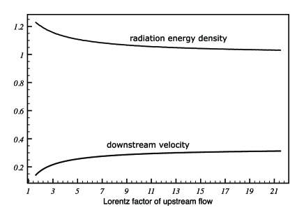
Figure 1: Velocity, $\beta_{d}$, and normalized radiation energy density, $e_{\gamma d}/(2m_{p}c^{2}n_{u}\gamma_{u}^{2}\beta^{2}_{u})$, of the downstream flow as functions of the upstream Lorentz factor $\gamma_{u}$.

3.2 Photon rich regime

As shown in Section 5, in photon rich shocks the density of pairs produced by nonthermal photons is typically much smaller than the density of the radiation, and while under certain conditions the pairs can dominate the opacity inside the shock and affect its structure, they contribute very little to the total energy budget downstream. The specific enthalpy is then well approximated by $w=nm_{p}c^{2}+4p_{\gamma}$, where $p_{\gamma}$ denotes the radiation pressure. Adopting the latter equation of state, the jump conditions, Equations (1)-(3), can be solved to yield the parameters of the downstream flow. Solutions for the downstream velocity, $\beta_{d}$, and the specific radiation energy, $e_{\gamma d}=3p_{\gamma d}$, are exhibited in Fig. 1 in the limit $\xi_{\gamma}\ll 1$. The radiation energy in Fig. 1 is normalized to the value obtained in the ultra-relativistic limit (i.e., for $\beta_{d}=1/3$):

$$e_{\gamma d}=2n_{u}\gamma_{u}^{2}\beta_{u}^{2}m_{p}c^{2}.$$ (13)

As seen, this asymptotic value is a good approximation also at mild Lorentz factors, and is adopted for illustration in the following discussion.

The downstream region of a RRMS is inherently non-uniform, because the thermalization length over which the plasma reaches full thermodynamic equilibrium is larger than the width of the shock transition layer. However, for typical astrophysical parameters, the thermalization length exceeds the shock width by several orders of magnitudes (Levinson, 2012), so that for any practical purpose photon generation in the downstream plasma can be ignored. This readily implies that to a good approximation the photon number is conserved across the shock transition layer, whereby

$$n_{\gamma d}\gamma_{d}\beta_{d}=n_{\gamma u}\gamma_{u}\beta_{u}.$$ (14)

Combining with Equation (1), one finds $\tilde{n}=n_{\gamma u}/n_{u}=n_{\gamma d}/n_{d}$. The temperature can be computed using Equations (13) and (14), yielding

$$\Theta_{d}=\frac{e_{\gamma d}}{3n_{\gamma d}\,m_{e}c^{2}}=\frac{2m_{p}}{3\,m_{e}}\frac{(\gamma_{u}\beta_{u})(\gamma_{d}\beta_{d})}{\tilde{n}}\simeq 430\,\frac{\gamma_{u}\beta_{u}}{\tilde{n}},$$ (15)

where $\beta_{d}=1/3$ was adopted to obtain the numerical factor in the rightmost term. Thus, $\Theta_{d}\ll 1$ as long as $\tilde{n}\gg 430\gamma_{u}\beta_{u}$.

Next, we estimate the minimum value of $\tilde{n}$ required in order that counter-streaming photons will be able to decelerate the upstream flow. Let $\eta$ denotes the fraction of downstream photons that propagate towards the upstream. The average energy each counter-streaming photon can extract in a single collision is at most $\gamma_{u}m_{e}c^{2}$. Thus, the number of downstream photons required to decelerate the upstream flow satisfies $\gamma_{d}\,n_{\gamma d}>\eta^{-1}(m_{p}/m_{e})\gamma_{u}\,n_{u}$ (assuming $\xi_{\gamma}\ll 1$). By employing Equation (14) we find that the shock can be mediated by the advected photons provided the photon-to-baryon number ratio far upstream satisfies

$$\tilde{n}>\tilde{n}_{crt}\equiv\frac{m_{p}}{m_{e}}\frac{\beta_{d}}{\eta\beta_{u}}\simeq\frac{m_{p}}{m_{e}},$$ (16)

adopting $\beta_{d}/\eta=1$, which is roughly the value obtained from the Monte-Carlo simulations. At the critical number density the average photon energy, $3kT_{d}\simeq 2\eta\,m_{e}c^{2}\gamma_{u}\beta_{u}$, is in excess of the electron mass. Under this condition a vigorous pair production is expected to ensue inside and just downstream of the shock, that will significantly enhance photon generation, thereby regulating the downstream temperature.

3.2.1 Analytic shock profile

Let $n_{\gamma\rightarrow u}$ denotes the density of photons moving in upstream direction (i.e., from downstream to the upstream), as measured in the shock frame, and $n$, $n_{e}$, $n_{\pm}$ the proper densities of baryons, electrons and $e^{\pm}$ pairs, respectively. We suppose that the flow moves along the $z$-axis, chosen such that its positive direction is towards the upstream. The change in the photon density is governed by the equation

$$\frac{dn_{\gamma\rightarrow u}}{dz}=-\sigma_{KN}\gamma(n_{e}+n_{\pm})n_{\gamma\rightarrow u}.$$ (17)

For sufficiently photon-rich shocks the scattering of bulk photons is in the Thomson regime. In terms of the optical depth, $d\tau_{*}=\sigma_{T}\,(n_{e}+n_{\pm})\gamma dz$, and the energy density of the counter streaming photons, $u_{\gamma\rightarrow u}=<\epsilon_{\gamma}>n_{\gamma\rightarrow u}$, one then has

$$\frac{du_{\gamma\rightarrow u}}{d\tau_{*}}=-u_{\gamma\rightarrow u}.$$ (18)

The total inverse Compton power emitted by a single electron (positron) inside the shock is approximately

$$P_{Comp}=\kappa_{\gamma}c\sigma_{T}(\gamma\beta)^{2}\,u_{\gamma\rightarrow u},$$ (19)

where the pre-factor $\kappa_{\gamma}$ ranges from $4/3$ for isotropic radiation to $4$ for completely beamed radiation. For simplicity, we shall assume that it is constant throughout the shock.

Neglecting the internal energy relative to baryon rest mass energy, the energy flux of the plasma can be expressed as

$$T_{b}^{0z}=m_{p}c^{2}n\gamma^{2}=J\gamma,$$ (20)

in terms of the conserved mass flux,

$$J=m_{p}c^{2}\,n\gamma.$$ (21)

Using Equation (19) we obtain

$$\frac{d\,T_{b}^{0x}}{dz} = \gamma(n_{e}+n_{\pm})c^{-1}P_{comp}$$

$$= \kappa_{\gamma}\sigma_{T}\,\gamma(n_{e}+n_{\pm})(\gamma^{2}-1)u_{\gamma\rightarrow u},$$

or

$$J\frac{d\,\gamma}{d\tau_{*}}=\kappa_{\gamma}(\gamma^{2}-1)u_{\gamma\rightarrow u}.$$ (23)

The boundary condition is $\gamma(\tau_{*}\rightarrow\infty)=\gamma_{u}$. Denoting $\alpha=\kappa_{\gamma}u_{\gamma\rightarrow u}(\tau_{*}=0)/J$, and

$$\eta(\tau_{*})=\ln\left(\frac{\gamma_{u}+1}{\gamma_{u}-1}\right)+2\alpha\,e^{-\tau_{*}}$$ (24)

the solution of Equations (18) and (23) reads:

$$\gamma(\tau_{*})=\frac{e^{\eta}+1}{e^{\eta}-1}.$$ (25)

From the jump conditions we have $\alpha=2\kappa_{\gamma}\epsilon\gamma_{u}$, where $\epsilon=u_{\gamma\rightarrow u}/u_{\gamma d}$ is roughly the fraction of downstream photons that propagate backwards. The black solid line in Fig. 2 shows the shock profile obtained for $\kappa_{\gamma}\epsilon=0.2$. The red line is the result of the full simulation.

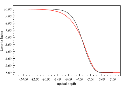
Figure 2: The solid black line delineates the solution given by Equation (25) with $\gamma_{u}=10$ and $\kappa_{\gamma}\epsilon=0.2$. The red line is the shock profile obtained from the Monte-Carlo simulation.

3.3 Photon starved regime

At $\tilde{n}<\tilde{n}_{crt}$ photon advection is negligible, and the prime source of photons inside and downstream of the shock transition layer is free-free emission. For sufficiently fast shocks, $\beta_{u}>0.6$, a pair production equilibrium is established downstream, keeping the temperature at $\Theta_{d}\lesssim m_{e}c^{2}/3$ (Katz et al., 2010). In relativistic shocks, $\gamma_{u}\gg 1$, the downstream photon density is obtained from Equation (13) and the relation $e_{\gamma d}\simeq m_{e}c^{2}n_{\gamma d}$’:

$$n_{\gamma d}\simeq 2\frac{m_{p}}{m_{e}}n_{u}\,\gamma_{u}^{2}.$$ (26)

This, in turn, implies that the transition from photon rich to photon starved shocks should in fact occur at $\tilde{n}\simeq\tilde{n}_{crt}\gamma_{u}$.

Because the average energy of downstream photons is roughly $m_{e}c^{2}$, scattering of counter streaming photons off electrons (positrons) in the shock transition layer is in the Klein-Nishina regime. As a consequence, the temperature at any position $z$ inside the shock is expected to be comparable to the local bulk energy of the leptons, specifically $\Theta(z)\simeq\gamma(z)$. Indeed, this result has been verified by detailed simulations (Budnik et al., 2010). When this relation is adopted it is possible to compute the shock structure analytically in the limit $\gamma_{u}\gg 1$ (Nakar & Sari, 2012; Granot, Nakar, & Levinson, 2017). The analysis indicates that the shock width increases with Lorentz factor according to

$$l_{s}^{\prime}\simeq 10^{-2}\gamma_{u}^{2}\,(\sigma_{T}n_{u})^{-1},$$

where the numerical coefficient is somewhat arbitrary (Nakar & Sari, 2012). This scaling stems from Klein-Nishina effects, and is different than the scaling obtained for photon rich shocks. The photon spectrum exhibits (in the shock frame) a peak at $h\nu_{peak}\simeq m_{e}c^{2}$, with a broad (a rough power law) extension up to energies $>\gamma_{u}m_{e}c^{2}$ (Budnik et al., 2010).

3.4 Effect of magnetic fields

Substantial magnetization of the upstream flow can significantly alter the shock profile and emission. A prominent feature of such shocks is the formation of a relatively strong subshock (Beloborodov, 2017). The results exhibited in Section 5 indicate that subshocks form also in unmagnetized shocks under certain conditions (see Figs. 6, 14 and 17), but those are generally weak and have little effect on the overall shock structure and emission, with the exception of the breakout transition, where photon leakage becomes important. In magnetized shocks formation of strong subshocks is anticipated even in regions of large optical depth, which can considerably alter the energy distribution of particles in the shock if particle acceleration at the collisionless subshock ensues. The net amount of energy that can be transferred to the nonthermal particles depends primarily on the relative strength of the subshock, and needs to be quantified. The formation of a strong subshock in RRMS may have profound implications for emission of sub-photospheric GRB shocks, as well as for neutrino production in chocked jets, as described above.

3.5 Finite shocks and breakout

The structures computed in Budnik et al. (2010) and in Section 5 are applicable to RRMS propagating in a medium of infinite optical depth. In cases where the shock propagates in a medium of gradually decreasing optical depth, e.g., stellar wind, it will eventually reach a point at which the radiation trapped inside it starts escaping to infinity. The leakage of radiation leads to a steepening of the shock, at least in photon starved RRMS. Nonetheless, the shock remains radiation mediated also at radii at which the optical thickness of the medium ahead of the shock is much smaller than unity, owing to self-generation of its opacity through accelerated pair creation. Breakout occurs when the Thomson thickness of the unshocked medium becomes smaller than $(m_{e}/m_{p})\gamma_{u}$, provided $\gamma_{u}>1$ , or else in the Newtonian regime (Granot, Nakar, & Levinson, 2017). How this affects the emitted spectrum is yet to be explored.

A similar process may take place also during the breakout of a photon rich shock, since photon escape from the medium ahead of the shock (i.e., the upstream plasma) is expected to lead to the gradual decline of $\tilde{n}$ over time. If pair creation and photon generation occur over a time shorter than the breakout time, then a transition from photon rich to photon starved shock is expected prior to breakout, at least in cases where the shock remains relativistic in the frame of the unshocked medium. Otherwise the shock will evolve in some complex manner. In any case, the spectrum emitted during the breakout phase may be altered.

4 Monte-Carlo simulations of RRMS

4.1 Description of the Monte-Carlo code

The Monte-Carlo code used by us enables computations of mildly relativistic and fully relativistic radiation mediated shocks in a planar geometry, for arbitrary upstream conditions. It incorporates an energy-momentum solver routine that allows adjustments of the shock profile in each iterative step. A photon source is placed sufficiently far upstream, and is tuned to account for the assumed photon density advected by the upstream flow. In each run, an initial shock profile is imposed (usually some parametrized analytic function that satisfies the shock jump conditions) during some initial stage at which photons that were injected upstream and crossed the shock are accumulated downstream. Once the photon density downstream reaches a level that ensures stability of the system, the energy-momentum solver is switched on, and the shock profile is allowed to change iteratively, until a steady state is reached whereby energy and momentum conservation of the entire system of particles (i.e., photons, baryons and electron-positron pairs) is satisfied at every grid point. Choosing the initial shock profile such that it satisfies the jump conditions in the frame of the simulation box guarantees that the final shock solution is stationary in this frame (otherwise it propagates across the box accordingly). Since the jump conditions depend only on the parameters of the upstream flow, they can be determined a-priori for any given set of upstream conditions.

The present version of the code includes the following radiation processes: Compton scattering, pair production and annihilation, and energy-momentum exchange with the bulk plasma. Its applicability is therefore restricted to photon rich shocks. We are currently in the process of incorporating also internal photon sources, specifically relativistic Bremsstrahlung and double Compton scattering, that would allow simulations of shocks for any upstream conditions, and in particular photon starved shocks. Magnetic fields can also be included upon a simple modification of the energy-momentum solver, and is planned for a future work.

In developing the prescription for the iteration in our code, we mimic the method used in the context of relativistic cosmic ray modified shocks (Ellison et al., 2013). The difference is that, while we track photons, they track cosmic rays using Monte-Carlo technique and evaluate the feedback on the bulk shock profile.

4.2 Numerical setup

In our calculations, the input parameters are the following quantities at the far upstream region: (i) the photon-to-baryon inertia ratio, $\xi_{u*}\equiv e_{\gamma u}/(n_{u}m_{p}c^{2})$, (ii) the photon-to-baryon number ratio, $\tilde{n}\equiv n_{\gamma u}/n_{u}$, and (iii) the bulk Lorentz factor of the upstream flow with respect to the shock frame, $\gamma_{u}$. Once these parameters are determined, all the physical quantities at the far upstream region are specified under the assumption that the radiation and the plasma (protons and electrons) have identical temperature, $T_{u}$. We further assume that the photons and the plasma constituents in the upstream region have Wien and Maxwell distributions, respectively. For given upstream conditions, we derive the corresponding steady shock solution using the iterative scheme described in the previous section.

In each iterative step, we solve the radiation transfer using Monte-Carlo method under a given plasma profile, and evaluate the energy-momentum exchange between the photon and plasma. We continue the iteration until the deviation of the total energy-momentum flux at every grid point from that of the steady state value becomes small. In the calculations presented in this paper, the errors in the conservation of momentum and energy fluxes after the iteration are mostly within a few % throughout the entire structure ($<15$ % at most). The total energy and momentum fluxes at each grid point are evaluated as

$$F_{m}=\gamma^{2}(\rho_{pl}c^{2}+e_{pl}+p_{pl})\beta^{2}+p_{pl}+F_{m,\gamma},$$ (27)

and

$$F_{e}=\gamma^{2}(\rho_{pl}c^{2}+e_{pl}+p_{pl})\beta+F_{e,\gamma},$$ (28)

respectively. Here $\rho_{\rm pl}=nm_{p}+(n+n_{\pm})m_{e}$, $e_{pl}=3/2nkT+3/2f(T)(n+n_{\pm})kT$, $p_{pl}=(2n+n_{\pm})kT$ are the rest mass density, internal energy density and pressure of the plasma, respectively, where $n_{\pm}$ is the number density of the created electron-positron pairs and $f(T)={\rm tanh}[({\rm ln}\Theta+0.3)/1.93]+3/2$ is an analytical function of temperature defined in Budnik et al. (2010), obtained from a fit to the exact equation of state of pairs at an arbitrary temperature ($f=1$ for $\Theta\ll 1$ and $f\approx 2$ for $\Theta\gg 1$). It is assumed that the protons and pairs have identical local temperature at every grid point. The last terms in the above equations, $F_{m,\gamma}$ and $F_{e,\gamma}$, denote the momentum and energy fluxes of radiation that are directly computed by summing up the contributions of individual photon packets tracked in the Monte-Carlo simulation. The steady state values of momentum, $F_{m,u}$, and energy fluxes, $F_{e,u}$, are evaluated by substituting the enthalpy $w_{u}=n_{u}(m_{p}+m_{e})c^{2}+[(7/2+3/2f(T_{u}))n+4n_{\gamma u}]kT_{u}$ and pressure $p_{u}=(2n+n_{\gamma})kT_{u}$ in the left side terms of Equations (2) and (3).

At first, the above iteration is performed under the assumption that a subshock is absent in the system. If it converges to steady flow, we simply employ the solution and consider that the shock dissipation is solely due to photon plasma interaction. On the other hand, when we find that the flow does not reach the steady state under the assumption (error in energy-momentum flux is larger than $\sim 20$ %), we introduce a subshock in the system. The subshock is treated as a discontinuity in the plasma profile which satisfies the Rankin-Hugoniot conditions under the assumption that bulk plasma is isolated from the radiation. This setup is justified due to the fact that, since the plasma scale is much shorter than that of the photon mean free path, photons cannot feel the continuous change in the transition layer of shock formed via plasma interactions. Once we introduce the subshock in the system, we also vary the immediate upstream velocity in each iterative steps and continue the computation until it approaches to steady solution.

Regarding the microphysical processes, Compton scattering is evaluated using the full Klein-Nishina cross section. It is noted that, in each scattering, bulk motion as well as thermal motion of the pairs are properly taken into account, under the assumption that the pairs have a Maxwellian distribution at the local temperature. The rate of pair production is calculated based on the local photon distribution using the cross section given in Gould & Schréder (1967). The pair annihilation rate is computed as a function of the local number density and temperature. Here we use the same analytical function employed in Budnik et al. (2010) which is based on the formula given by Svensson (1982). As for the spectra of photons generated via the pair annihilation process, we employ an analytical formula derived in Svensson et al. (1996) which is given as a function of temperature. The details of the processes incorporated in our code are summarized in the appendix.

In this study we systematically explore the properties of RRMS, with a particular focus on the role of the three parameters defined above. We performed 15 model calculations that cover a wide range of parameters ($10^{-2}\leq\xi_{u*}\leq 10$, $10^{3}\leq\tilde{n}\leq 10^{5}$, and $2\leq\gamma_{u}\leq 10$). Table 1 summarizes the imposed values for each calculation. The total number of injected photon packets varies among the models, but is typically in the range $N_{\rm pack}\sim 10^{8}-10^{9}$, which is sufficiently large to avoid significant statistical errors.

Table 1: Shock Parameters. Column (1) shows the names of the models. Columns (2), (3) and (4) display, respectively, the bulk Lorentz factor, photon-to-baryon inertia ratio, and photon-to-baryon number ratio at far upstream.

Model	$\gamma_{u}$	$\xi_{u*}$	$\tilde{n}$
(1)	(2)	(3)	(4)
g2e1n5		10
g2e0n5	2	1	$10^{5}$
g2e-1n5		$10^{-1}$
g2e-2n5		$10^{-2}$
g2e0n4		1
g2e-1n4	2	$10^{-1}$	$10^{4}$
g2e-2n4		$10^{-2}$
g2e-1n3	2	$10^{-1}$	$10^{3}$
g2e-2n3		$10^{-2}$
g4e0n5		1
g4e-1n5	4	$10^{-1}$	$10^{5}$
g4e-2n5		$10^{-2}$
g10e0n5		1
g10e-1n5	10	$10^{-1}$	$10^{5}$
g10e-2n5		$10^{-2}$

5 Results

In this section, we demonstrate how the different parameters affect the shock properties. Hereafter we refer to the models with $\gamma_{u}=2$ and $\tilde{n}=10^{5}$ as fiducial cases (g2e1n5, g2e0n5, g2e-1n5 and g2e-2n5), since such conditions are likely to prevail in sub-photospheric GRB shocks. Note that the cases $\xi_{u*}\geq 1$ and $\xi_{u*}<1$ correspond to shocks formed below and above the saturation radius, respectively, in the context of the fireball model.

5.1 Dependence on $\xi_{u*}$

As for the fiducial models ($\gamma_{u}=2$ and $\tilde{n}=10^{5}$), we compute the cases for $\xi_{u*}=10,1,0.1$, and $10^{-2}$. The obtained shock structures are displayed in Fig. 3. The horizontal axis in all plots shows the angle averaged, pair loaded optical depth for Thomson scattering, as measured in the shock frame:

$$\tau_{*}=\int\gamma(n+n_{\pm})\sigma_{T}dz,$$ (29)

where $dz$ denotes the distance element along the flow direction. It is measured from the subshock, when present, where $\tau_{*}=0$, and from the location where the bulk velocity has first reached the far downstream value, $\beta\simeq\beta_{d}$, when the subshock is absent. As a function of $\tau_{*}$, the vertical axis shows the 4-velocity, $\gamma\beta$, temperature, $T$, and the pair-to-baryon density ratio, $n_{\pm}/n$. Together with the plasma temperature, we also display the quantity

$$T_{\gamma,eff}=\frac{I_{0}^{{}^{\prime}}}{3{\cal I}_{0}^{{}^{\prime}}}$$ (30)

for reference, where $I_{0}$ and ${\cal I}_{0}$ are, respectively, the 0th moments of the intensity $I_{\nu}$ and the photon flux density $I_{\nu}/h\nu$. Henceforth, quantities with and without the superscript prime are measured in the comoving frame and shock frame, respectively. The $n$th moments of the intensity and photon flux density are defined as follows:

$$I_{n}=2\pi\int\int I_{\nu}{\rm cos}^{n}\theta~{}d\nu d\Omega,$$ (31)

$${\cal I}_{n}=2\pi\int\int\frac{I_{\nu}}{h\nu}{\rm cos}^{n}\theta~{}d\nu d\Omega,~{}~{}~{}(n=0,1,2),$$ (32)

where $\theta$ is the angle between the flow velocity and the photon direction. Note that $T_{\gamma,eff}$ can be regarded as the actual temperature of the radiation when the distribution is Wien, $I_{\nu}\propto\nu^{3}{\rm exp}[h\nu/(kT)]$, or Planck. Henceforth, we refer to $T_{\gamma,eff}$ as the effective radiation temperature. The angle integrated spectral energy distribution (SED), $\int\nu I_{\nu}d\Omega$, computed in the shock frame at a given location, is exhibited in Fig. 4 for each model at different locations. In Fig. 5 we show a comparison of the 4-velocity profiles of the different fiducial models, together with the comoving 1st and 2nd moments of the radiation intensity normalized by the 0th moment, $I_{1}^{{}^{\prime}}/I_{0}^{{}^{\prime}}$ and $I_{2}^{{}^{\prime}}/I_{0}^{{}^{\prime}}$. When the radiation field is isotropic in the comoving frame, we have $I_{2}^{{}^{\prime}}/I_{0}^{{}^{\prime}}=1/3$ and $I_{1}^{{}^{\prime}}=0$, while completely beamed radiation leads to $I_{2}^{{}^{\prime}}/I_{0}^{{}^{\prime}}=1$ and $I_{1}^{{}^{\prime}}/I_{0}^{{}^{\prime}}=-1$ or $1$.

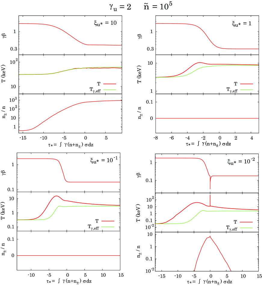
Figure 3: The overall shock structure for models g2e1n5 (top left), g2e0n5 (top right), g2e-1n5 (bottom left) and g2e-2n5 (bottom right). In each panel, from top to bottom, we display the 4-velocity $\gamma\beta$, the plasma temperature $T$, the effective radiation temperature $T_{\gamma,{\rm eff}}$, and the pair -to- baryon density ratio $n_{\pm}/n$, as a function of optical depth $\tau_{*}$. Note the difference in the scaling of the horizontal and vertical axes in the different models.

Figure 4: Shock-frame, local angle integrated SEDs, $\int\nu I_{\nu}(\tau*)d\Omega$, for models g2e1n5 (top left), g2e0n5 (top right), g2e-1n5 (bottom left) and g2e-2n5 (bottom right). The red and black lines show, respectively, the spectra near the upstream and downstream boundaries of the simulation domain. The value of $\tau_{*}$ at the boundaries vary among the different models. The green, blue, magenta, cyan and gray lines display spectra which were computed at locations $\tau_{*}=-2$, $-1$, $0$, $1.5$ and $2.5$ around the shock transition layer, as indicated. The scale on the vertical axis is given in arbitrary units. The absolute value can be specified once the number density of either baryons or photons at far upstream ($n_{u}$ or $n_{\gamma,u}$) is specified. Note that the range of the horizontal axis is identical in all cases.

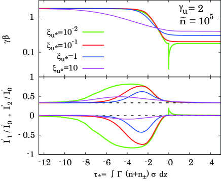
Figure 5: Dependence of the 4-velocity profile (top) and the normalized comoving 1st and 2nd moments of the radiation intensity, $I_{1}^{{}^{\prime}}/I_{0}^{{}^{\prime}}$ and $I_{2}^{{}^{\prime}}/I_{0}^{{}^{\prime}}$ (bottom), on the far upstream photo-to-baryon inertia ratio $\xi_{u*}$, for $\gamma_{u}=2$ and $\tilde{n}=10^{5}$. The green, red, blue and magenta lines correspond to models g2e-2n5, g2e-1n5, g2e0n5 and g2e1n5, respectively. For a given pair of lines in each model in the bottom panel, the upper one corresponds to the second moment $I_{2}^{{}^{\prime}}/I_{0}^{{}^{\prime}}$, and the lower one to the first moment $I_{1}^{{}^{\prime}}/I_{0}^{{}^{\prime}}$. The two dashed lines in the bottom panel mark the values of the radiation moments of an isotropic radiation field ($I_{1}^{{}^{\prime}}/I_{0}^{{}^{\prime}}=0$ and $I_{2}^{{}^{\prime}}/I_{0}^{{}^{\prime}}=1/3$).

Although there is some difference between the models, the deceleration of the shock occurs over an optical depth $\tau*$ of a few in all cases. This stems from the fact that in the relativistic case the plasma crossing time of the shock is nearly equal to the light crossing time. The relativistic motion of the plasma is also the sole reason why inside the shock transition layer the radiation appears highly anisotropic in the rest frame of the fluid, as seen in Fig. 5. As mentioned in Section 1, this is in marked difference to non-relativistic shocks in which the diffusion length is much longer, and the radiation is nearly isotropic. During the deceleration, Compton scattering also heats up the plasma to higher temperatures. Regarding the radiation spectra, while a Wien distribution at the local temperature is established at the far upstream and downstream regions, non-thermal distributions originating from bulk Comptonization are produced near the shock transition layer. Apart from these general trends, the details of shock dissipation vary considerably with $\xi_{u*}$.

In model g2e1n5, the inertia of the flow at far upstream is largely dominated by the radiation ($\xi_{u*}=10$). In this case, strong anisotropy cannot develop within the shock, since a small departure from isotropy is sufficient to give significant impact on the bulk flow of the plasma. As a result, the velocity profile is relatively smooth, reflecting gradual deceleration compared with the cases of lower $\xi_{u*}$. As shown in Beloborodov (2017), in the extreme limit of $\xi_{u*}=\infty$, the radiation field must satisfy the force-free condition $I_{1}^{{}^{\prime}}=0$. Here (model g2e1n5) the plasma has a finite contribution to the inertia ($\sim 10\%$ of the total), therefore a small but finite anisotropy is present.

In this model, the temperature of the plasma coincides with the effective temperature of the radiation, $T_{\gamma,eff}$, at any position. This is due to the fact that the photon distribution is close to Wien, so that Compton equilibrium (see Section C for details) is established throughout the shock. The spectra of photons do not largely depart from the Wien distribution because bulk Comptonization, which mediates the shock, need not be significant. The resulting temperature shows gradual increase from $kT\sim 30~{}{\rm keV}$ to $\sim 60~{}{\rm keV}$ across the deceleration zone (see upper left panel of Fig. 3). Although the change in the temperature is only a factor of $\sim 2$ across the shock, significant increase is found in the pair number density. This is because the pair production rate by photons in a Wien distribution is a sensitive function of temperature in this range ($kT\sim 30-60\,{\rm keV})$, since only the high energy population around the exponential cutoff exceeds the threshold energy for pair creation. As a result, the pair loading, $n_{\pm}/n$, increases by three orders of magnitude across the transition layer. At the far upstream and downstream regions, pair production and annihilation are in balance and the number density of pairs can be well approximated by that of Wien equilibrium at non-relativistic temperatures (see Section B.1). From Equation (59) ($n_{\pm}/n\sim\tilde{n}\Theta^{-3/2}{\rm exp}(-\Theta^{-1})$), we obtain $n_{\pm}\sim 0.35$ ($n_{\pm}\sim 6.2\times 10^{2}$) for a far upstream (downstream) temperature of $kT\sim 30~{}{\rm keV}$ ($\sim 60{\rm keV}$). Indeed, this is in good agreement with our simulation.

As the value of $\xi_{u*}$ decreases, the velocity gradient, $d\gamma\beta/d\tau_{*}$, steepens. This is mainly due to the fact that for a given density ratio $\tilde{n}$, the average energy of photons decreases with decreasing $\xi_{u*}$, since the upstream temperature satisfies $T_{u}\propto\xi_{u*}$. As a result, Klein-Nishina effects are diminished, and the average mean free path of photons is reduced, ultimately approaching the Thomson limit. A steeper velocity gradient is also required for lower values of $\xi_{u*}$ in order to increase the efficiency at which the bulk kinetic energy is extracted by bulk Comptonization. As shown in Fig. 4, when the photon-to-baryon inertia ratio is reduced to the value $\xi_{u*}=10^{-2}$ (model g2e-2n5), a smooth velocity profile is no longer sufficient to achieve energy-momentum conservation to the required accuracy at every grid point, and our calculations imply the formation of a subshock in the system. It is noted, however, that the subshock is quite weak, in the sense that it carries only a small fraction (a few percents at most) of the entire shock energy, and so do not play an important role in the dissipation process. Therefore, its impact on the radiation properties is also negligible. Therefore, in what follows we mainly focus on the global properties of the shock, that are not affected by the subshock. The details of the subshock structure will be given later on, in Section 5.1.1.

The bulk Comptonization in the deceleration zone becomes significant as $\xi_{u*}$ decreases, and results in the emergence of a non-thermal spectrum. As shown in Fig. 4, the spectral slope is harder for smaller values of $\xi_{u*}$. Concomitant with the hardening of the spectrum, the departure from isotropy (as seen in the comoving frame) that develops inside the shock becomes more prominent (bottom panel of Fig. 5).

The maximum energy attainable through bulk Comptonization is limited by the kinetic energy of the electrons/positrons to about $(\gamma_{u}-1)m_{e}c^{2}\sim 500~{}{\rm keV}$. When the pair content is small, this corresponds roughly to the cutoff energy of the non-thermal photons at high energies (e.g., models g2e0n5 and g2e-1n5). On the other hand, when gamma ray production via pair annihilation is important, the conversion of rest mass energy leads to a moderate increase in the cutoff energy, roughly to $\gamma_{u}m_{e}c^{2}\sim 1~{}{\rm MeV}$ (e.g., model g2e-2n5). Also note that, although the temperature is non-relativistic, thermal motions slightly shift the energy to higher values and produce a broadening of the spectrum at the highest energies (Fig. 4).

Since Compton equilibrium is achieved throughout the shock (except for the immediate post subshock region), as explained in Section C, and higher energy photons can exchange their energy more efficiently via scattering, the presence of non-thermal photons will result in an abrupt heating of the plasma up to a temperature well in excess of $T_{\gamma,eff}$. Therefore, while no departure is found for model g2e1n5 ($T\sim T_{\gamma,eff}$), the deviation of the plasma temperature from $T_{\gamma,eff}$ becomes more substantial as $\xi_{u*}$ decreases (see Fig. 3). This implies the presence of a prominent plasma heating precursor at the onset of the shock transition layer for relatively low values of $\xi_{u*}$.

The pair density profile also changes significantly with $\xi_{u*}$. While there is a significant amount of pairs in model g2e1n5, they are negligible in models g2e0n5 and g2e-1n5 ($n_{\pm}/n\ll 10^{-10}$). This is a direct consequence of the lower peak energy (approximately $3kT_{\gamma,eff}$), that gives rise to an exponential suppression of the number of photons above the pair creation threshold. On the other hand, while $T_{\gamma,eff}$ is still low, the production of a prominent non-thermal component leads to enhanced pair production in model g2e-2n5. The pairs only appear in the vicinity of the transition layer, since the pair production opacity contributed by the bulk Comptonized photons peaks there.

It should be noted that the existence of pairs can change the spatial width of the shock considerably once their density exceeds the baryon density ($n_{\pm}/n\gtrsim 1$) and begins to govern the scattering opacity inside the shock. For example, the physical length scale per optical depth $dz/d\tau_{*}$ at far upstream is longer than that of the far down stream by roughly 3 orders of magnitude. Therefore, one should bear in mind that, while the shock width in terms of $d\tau_{*}$ is similar among the models, it could largely differ when measured in terms of the physical length scale $dz$, even when the same far upstream density $n_{u}$ is invoked.

5.1.1 Emergence of a weak subshock

As mentioned earlier, emergence of a weak subshock seems necessary in model g2e-2n5. Although its contribution to the overall dissipation is quite small, its existence is required to achieve steady flow solutions (see Section 4.2 for details). As described in Section 4.2, we treat the subshock as a discontinuity in the flow parameters that satisfy the Rankin-Hugoniot condition for a plasma isolated from the radiation. A notable feature of the subshock is a sharp spike followed by a dip in the velocity and temperature profiles. The drop in the velocity to a value smaller than the far downstream velocity is an inevitable consequence of the plasma sound speed, $c_{s}\approx[5P_{pl}/3\rho_{pl}]^{1/2}$, being small ($c_{s}/c\sim 0.09$ for $kT\sim 500~{}{\rm keV}$ and $n{\pm}/n\sim 10$). The rise of the temperature just behind the subshock, up to $kT_{d,sub}\sim 500~{}{\rm keV}$, is caused by the self-generated heat of the plasma within the subshock. Since the photons cannot interact with particles over the plasma scale, the post shock temperature is well above that obtained in Compton equilibrium. Consequently, following shock heating, the pairs exposed to the intense radiation field rapidly cool via Compton scattering until the temperature reaches the equilibrium value (roughly equals to that ahead of the subshock). As a result, a structure that resembles an isothermal shock is formed (see a magnified view in Fig. 6). Within the cooling layer ($\tau_{*}\lesssim 0.001$), the bulk plasma rapidly accelerates, predominantly by its pressure gradient force. Above the cooling layer, the acceleration continues more gradually, mainly due to the radiation force, up to the distance where it reaches the far downstream velocity (at $\tau_{*}\sim 0.6$)

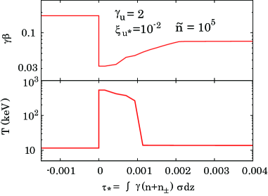
Figure 6: Enlarged view of the 4-velocity and temperature profiles around the weak subshock, for model g2e-2n5.

A crude evaluation of the thickness of the cooling layer, $d\tau_{*,cool}$, can be derived as follows: The number of scatterings per unit time for a single electron/positron is given by $\sim n_{\gamma}c\sigma_{T}$ in the comoving frame. Hence, given the energy loss per scattering, $\sim 4<h\nu>kT_{d,sub}/m_{e}c^{2}$, and the downstream thermal energy per electron/positron, $3kT_{d,sub}$, the cooling time is derived as $t_{cool}\sim 3/4(<h\nu>/m_{e}c^{2})^{-1}(n_{\gamma}c\sigma_{T})^{-1}$, where $<h\nu>$ and $kT_{d,sub}$ denote the average photon energy and the temperature at the immediate downstream of the subshock. In terms of the effective temperature, the average photon energy at the subshock can be expressed as $<h\nu>\sim 3kT_{\gamma,eff}$. While the photon number density is approximately $n_{\gamma}\sim\tilde{n}n$ over most of the RRMS layer, it is given by $n_{\gamma}\sim\tilde{n}n\beta_{u,sub}/\beta_{d,sub}$ at the immediate downstream of the subshock, owing to the sudden compression of the plasma there, where $\beta_{u,sub}$ ($\beta_{d,sub}$) is the velocity at the immediate upstream (downstream) of the subshock. Taking into account the above factors, the cooling layer thickness can be expressed as

$$d\tau_{*,cool} \sim \beta_{d,sub}c(n+n_{\pm})\sigma_{T}t_{cool}$$

$$\sim 1.5\times 10^{-3}\left(\frac{kT_{\gamma,eff}}{2~{}{\rm keV}}\right)^{-1}\left(\frac{\tilde{n}}{10^{5}}\right)^{-1}\left(\frac{\frac{n+n_{\pm}}{n}}{10}\right)$$

$$~{}~{}~{}~{}~{}~{}~{}~{}~{}~{}\times\left(\frac{\frac{\beta_{u,sub}}{\beta_{d,sub}}}{8}\right)\left(\frac{\beta_{d,sub}}{0.03}\right).$$

Pair creation and annihilation were ignored in the above derivation, as they are negligible over the cooling layer given its small thickness relative to the entire RRMS transition layer (see bottom right panel of Fig. 3).

We can confirm from Fig. 6 (as well as from Figs. 9, 14 and 17 for the other models with subshocks) that this rough estimation is in agreement with our numerical results within a factor of a few. Note that there are several factors that were ignored in our crude estimation of the cooling layer thickness, and which can lead to some differences between the analytic and numerical results. For example, we have neglected the effect of adiabatic cooling as well as the effect of broad radiation spectrum. Moreover, in evaluating the cooling rate, we have used an expression which is only valid in the non-relativistic limit, $kT_{u,sub},kT_{d.sub}\ll m_{e}c^{2}$, while the temperature is typically mildly relativistic. In view of these simplifications, we find the mild disagreement between the numerical result and the analytic result derived above reasonable.

It is worth noting that, while this weak subshock strongly affects the properties of the plasma in its vicinity, it has almost no influence on the radiation. This is simply because the thermal energy generated by the subshock, $3(n+n_{\pm})kT_{d,sub}$, is negligible compared with that contained in the radiation, $3n_{\rm\gamma}kT_{\gamma,eff}$. Therefore, the weak subshock does not affect the overall energetics of the system nor the radiation properties. This is also true for all the other cases in which subshocks were found, and for which the photon-to-baryon number ratio is sufficiently above the critical value $\tilde{n}_{crt}$ given in Equation (16) (see Section 3.2).

While our numerical simulations predict their existence, we could not identify the physical origin of the “weak” subshocks that we found in the regime $\tilde{n}\gtrsim n_{crt}$ (models g2e-2n5, g4e-2n5, g10e-1n5 and g10e-2n5), unlike the case of a photon starved shock, $\tilde{n}<n_{crt}$ (models g2e-1n3 and g2e-2n3), where formation of a “strong” subshock is dictated by inefficient energy extraction thorough Compton scattering, as will be discuss in greater detail in Section 5.2 below. Though non trivial, this presumably indicates that no steady, continuous flow solutions exist in a certain regime of the parameter space. As seen in Fig. 5, the flow velocity gradient tends to steepen as the value of $\xi_{u*}$ is reduced. Our result suggests that there is a threshold value of $\xi_{u*}$ below which the continuous steepening of the velocity profile ultimately turns into a weak subshock at the edge of the RRMS transition layer. It is worth mentioning that Budnik et al. (2010) also found a weak subshock in their simulations of photon starved RRMS (in which photon generation is included). It should be stressed, however, that these weak subshocks are merely small disturbances in the global shock structure, and their physics is not important in evaluating the overall dynamics of the bulk flow as well as the radiation properties.

5.2 Dependence on $\tilde{n}$

To explore the dependence of the shock properties on the photon-to-baryon number ratio, we performed several calculations that invoke smaller values of $\tilde{n}$ ($10^{4}$ and $10^{3}$) than that used in the fiducial models, but the same values of $\gamma_{u}$ and $\xi_{u*}$. In the models with $\tilde{n}=10^{4}$, three cases with different values of photon-to-baryon inertia ratio ($\xi_{u*}=1$, $0.1$ and $0.01$) are considered (g2e0n4, g2e-1n4 and g2e-2n4). Their overall structures and spectra are summarized in Figs. 7 and 8. As seen, the general trends are quite similar to those of the fiducial models; the decrease in $\xi_{u*}$ results in a steepening of their velocity gradient $d\gamma\beta/d\tau_{*}$ and in the enhancement of the non-thermal spectrum.

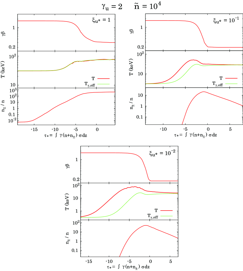
Figure 7: Same as Fig. 3, but for g2e0n4 (top left), g2e-1n4 (top right) and g2e-2n4 (bottom).

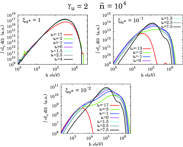
Figure 8: Same as Fig. 4, but for g2e0n4 (top left), g2e-1n4 (top right) and g2e-2n4 (bottom).

Apart from the similarities, there are also interesting differences from the fiducial models ($\tilde{n}=10^{5}$). For a fixed value of $\xi_{u*}$, lower $\tilde{n}$ results in a higher temperature ($T\propto\tilde{n}^{-1}$), since the same amount of energy is shared by a smaller number of particles (photons, protons and pairs). Hence, the overall temperature and average photon energy are roughly $10$ times higher in these models. This shifts the average mean free path of photons to larger values owning to the increase in the population of photons that are scattered in the Klein-Nishina regime. As a result, the deceleration lengths are found to be longer than those in the corresponding fiducial models (g2e0n5, g2e-1n5, g2e-2n5). The higher temperature and photon energy are probably the reason for the absence of a weak subshock in model g2e-2n4, in difference from model g2e-2n5 (that has the same $\xi_{u*}$ value). We speculate that the smoother velocity profile in model g2e-2n4, that results from the larger penetration depth of the photons, enables the existence of steady solutions with no subshock. However, it is expected that a weak subshock will form also in these models for sufficiently low values of $\xi_{u*}$ ($<0.01$).

The larger temperature or, equivalently, average photon energy, also leads to enhanced pair production rate. In particular, while the pair content is negligible for $\xi_{u*}=1$ and $\xi_{u*}=0.1$ in the fiducial models (g2e0n5 and g2e-1n5), the models with $\tilde{n}=10^{4}$ and the same $\xi_{u*}$ values (g2e0n4 and g2e-1n4) give rise to a significant amount of pairs. Likewise, the pair density in model g2e-2n4 is higher by an order of magnitude than that in the fiducial model g2e-2n5.

Comparing the structures, the profiles in model g2e0n4 are similar to those in model g2e1n5, rather than in model g2e0n5 that has the same $\xi_{u*}$ value. Accordingly, as in model g2e1n5, the radiation and pairs are well approximated to be in Wien equilibrium at far upstream and downstream, while the in the transition layer they depart from the equilibrium due to a slight deviation from the Wien distribution. On the other hand, the shape of the spectrum in models g2e-1n4 and g2e-2n4 is similar to that of the counterpart fiducial models with same $\xi_{u*}$ (g2e-1n5 and g2e-2n5), but its average energy is shifted toward higher energies, by a factor of $\sim 10$, while the cutoff energy remains unchanged $\sim\gamma_{u}m_{e}c^{2}\sim 1~{}{\rm MeV}$. The higher photon energies in models g2e-1n4 and g2e-2n4 give rise to a higher pair production rate than in the fiducial models. Therefore, in all of these models, we find a non-negligible pair content.

The properties of the shocks drastically change in the models with $\tilde{n}=10^{3}$. In the present study, two cases with the values $\xi_{u*}=0.1$ and $0.01$ are computed (g2e-1n3 and g2e-2n3). Their overall structures and spectra are exhibited in Figs. 9 and 10, respectively. The notable difference from the models with higher $\tilde{n}$ is the formation of a “strong” subshock. Unlike the “weak” subshocks found in some of the other models (see Section 5.1.1 for details), the physical origin of the strong subshocks is understood, and will be described in detail in Section 5.2.1.

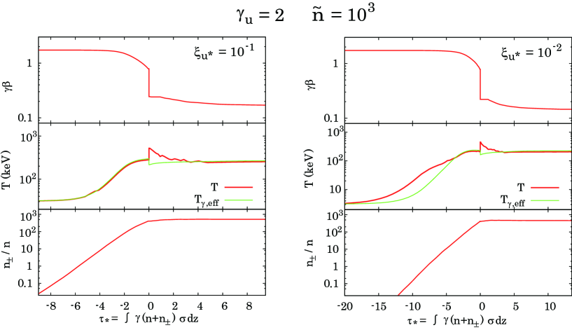
Figure 9: Same as Fig. 3, but for g2e-1n3 (left) and g2e-2n3 (right).

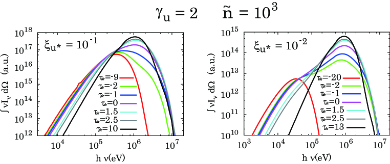
Figure 10: Same as Fig. 4, but for g2e-1n3 (left) and g2e-2n3 (right).

As Equation (15) predicts, the temperature downstream of the subshock in the models with $\tilde{n}=10^{3}$ approaches the pair equilibrium value, $kT\sim 200~{}{\rm keV}$, as seen in Fig. 9. The pair density increases rapidly inside the shock and approaches the Wien equilibrium value, $n_{\pm}\approx n_{\gamma}K_{2}(\Theta^{-1})/\Theta^{2}$, just downstream of the subshock. At this temperature the pair density becomes comparable to the photon density, $n_{\pm}\sim n_{\gamma}$. Since in the absence of an internal photon source the number of quanta is conserved, we have $\tilde{n}=(n_{\gamma}+n_{\pm})/n$ in the downstream region, which effectively reduces the number of photons that can extract energy, and strengthens the subshock further. One should keep in mind that while the subshock is relatively strong, it dissipates only about 30% of the entire shock energy (in model g2e-2n3). Thus, a moderate increment in the photon density downstream (by no more than a factor of a few) will considerably weaken, or completely eliminate, the subshock. We anticipate this to happen once internal photon sources (in particular free-free emission by the hot pairs) are included.

Shock solutions that correspond to the fiducial models with fixed $\xi_{u*}=0.1$ are compared, for clarity, in Fig. 11. The distinct properties of the marginally starved shock (g2e-1n3) stand out. The discontinuity in the profiles of the moments $I_{1}^{{}^{\prime}}/I_{0}^{{}^{\prime}}$ and $I_{2}^{{}^{\prime}}/I_{0}^{{}^{\prime}}$ in the marginally starved shock arises from the sudden change in the velocity of fluid elements (and, hence, in the frame in which these moments are computed) across the subshock.

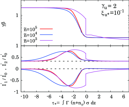
Figure 11: Same as Fig. 5, but for models g2e-1n5 (red), g2e-1n4 (blue) and g2e-1n3 (magenta).

5.2.1 Transition to the photon starved regime

Next, let us examine the transition from the photon rich to the photon starved regime in some greater detail. In section 3.2 it has been argued that once the photon-to-baryon number ratio far upstream becomes smaller than the critical value $\tilde{n}_{crt}$, the advected photons cannot support the shock anymore, and the shock becomes photon starved. In the absence of photon production processes one expects that the strength of the subshock will dramatically increase as $\tilde{n}$ approaches $\tilde{n}_{crt}\simeq 10^{3}$. This is the situation in models g2e-1n3 and g2e-2n3. Fig. 9 exhibits results obtained for these models, verifying that the subshock is indeed substantially stronger than in the runs with $\tilde{n}>\tilde{n}_{crt}$. As also seen, the downstream temperature reaches $200$ keV (except for the spike produced by the subshock), in accord with Equation (15), leading to a vigorous pair creation in the shock transition layer. The pair-photon plasma downstream quickly reaches equilibrium, with roughly equal densities, $n_{\pm}/n_{\gamma}\simeq 1$.

From Equation (3.1) it is anticipated that under these conditions photon generation (not included in our simulations) will start dominating over photon advection, so that in reality the shock will be supported by photons produced inside and just behind the shock, and the subshock will disappear or remain insignificant. For higher upstream Lorentz factors, $\gamma_{u}\gg 1$, we expect that photon generation will dominate at somewhat higher $\tilde{n}$ values, roughly by a factor of $\gamma_{u}/2$, since even though the shock can be supported by the advected photons the temperature downstream exceeds the pair production threshold, at which e^± pair equilibrium is established. The results of Budnik et al. (2010) confirm this. We are currently in the process of modifying the code to include free-free and double Compton emissions. Results of simulations of photon starved shocks will be presented in a future publication.

5.3 Dependence on $\gamma_{u}$

To investigate the dependence of the shock properties on the Lorentz factor, we have calculated two sets of models with higher $\gamma_{u}$ ($4$ and $10$), but with the values of $\tilde{n}$ and $\xi_{u*}$ being identical to those in the fiducial models. In both cases, three calculations that invoke different $\xi_{u*}$ values ($1$, $0.1$ and $0.01$) were performed, and are described next.

The structures and spectra obtained in the models with $\gamma_{u}=4$ and $\gamma_{u}=10$ are displayed in Figs. 12 - 17. Like in the fiducial models, also here the velocity profile steepens as $\xi_{u*}$ is reduced. The trends of the temperature profile are also similar to those in the fiducial models, albeit with a higher downstream temperature, since it is roughly proportional to the 4-velocity far upstream when $\xi_{u*}\lesssim 1$ (see Equation (15)). At low values of $\xi_{u*}$ a weak subshock appears (see Figs. 14 and 17 for a magnified view), as in the fiducial models. The larger $\gamma_{u}$ the larger the value of $\xi_{u*}$ at which the subshock forms ($\xi_{u*}\leq 0.01$ for $\gamma_{u}=4$ and $\xi_{u*}\leq 0.1$ for $\gamma_{u}=10$). The reason for this is unclear at present. It might be related to the fact that the condition for starvation is proportional to $\gamma_{u}$ (see Equation (26) ).

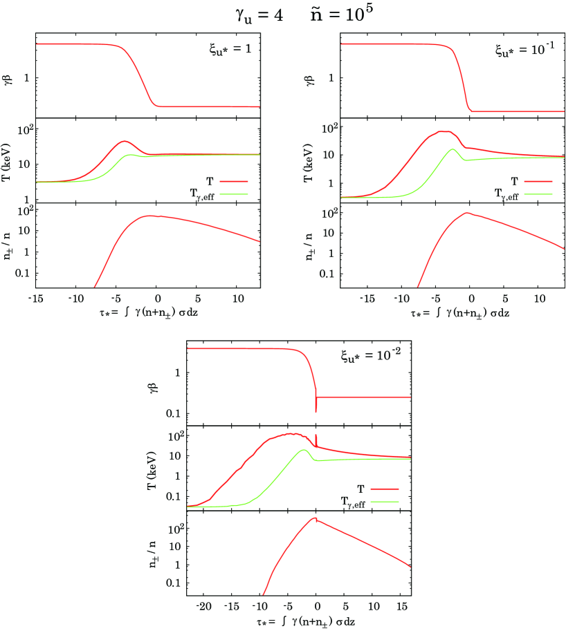
Figure 12: Same as Fig. 3, but for g4e0n5 (top left), g4e-1n5 (top right) and g4e-2n5 (bottom).

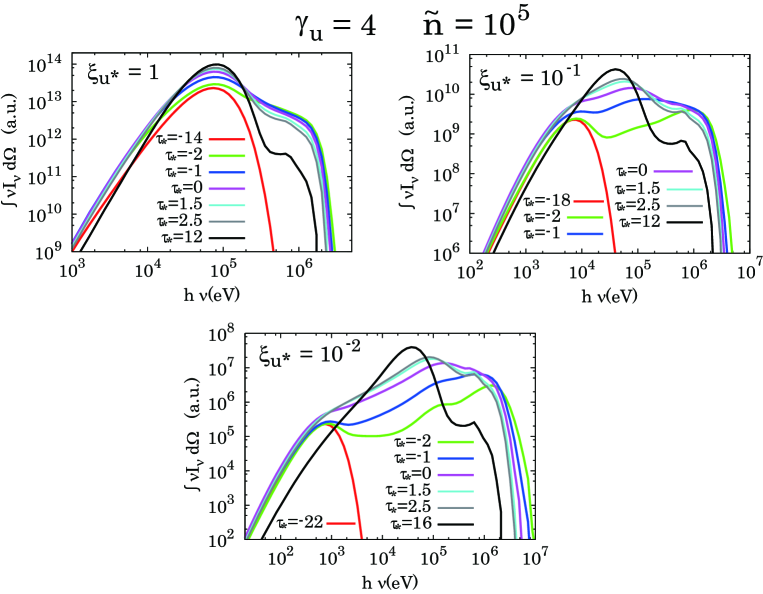
Figure 13: Same as Fig. 4, but for g4e0n5 (top left), g4e-1n5 (top right) and g4e-2n5 (bottom).

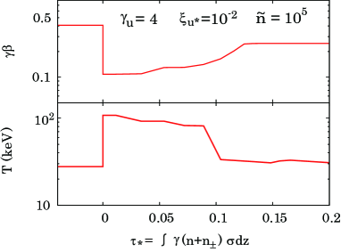
Figure 14: Enlarged view of the 4-velocity and temperature profiles around the weak subshock region for model g4e-2n5.

The main effects caused by increasing the shock Lorentz factor can be observed in the resulting spectra and pair populations, and can be summarized as follows: (i) The heating precursor broadens and the peak temperature increases as $\gamma_{u}$ increases, and likewise the width of the shock transition layer. (ii) The pair content rises sharply as $\gamma_{u}$ increases, as is evident from a comparison of Figs. 12 and 15. This is a direct consequence of the fact that the number of bulk Comptonized photons that surpass the pair production threshold and, hence, the pair production rate, are sensitive functions of $\gamma_{u}$. The large pair enrichment gives rise to a pronounced signature of the $511~{}{\rm keV}$ pair annihilation line in the spectrum (the small spectral bumps seen in Figs. 13 and 16). (iii) For fixed values of $\tilde{n}$ and $\xi_{u*}$ the high energy cutoff of the spectrum is roughly proportional to $\gamma_{u}$, as naively expected.

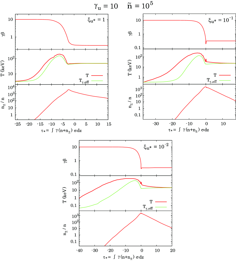
Figure 15: Same as Fig. 3, but for g10e0n5 (top left), g10e-1n5 (top right) and g10e-2n5 (bottom).

Figure 16: Same as Fig. 4, but for g10e0n5 (top left), g10e-1n5 (top right) and g10e-2n5 (bottom).

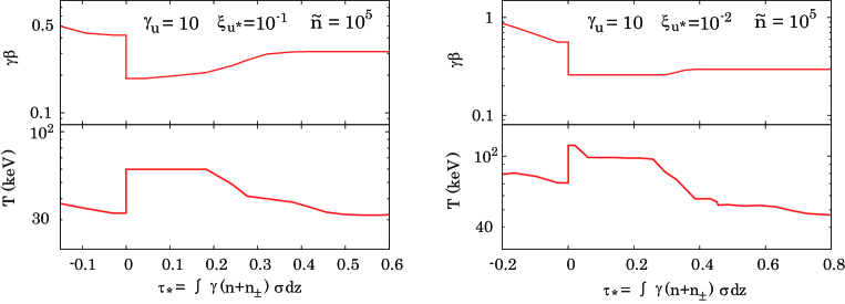
Figure 17: Enlarged view of 4-velocity and temperature profile around the weak subshock region for model g10e-1n5 and g10e-2n5.

To summarize the dependence of the shock structure on the bulk Lorentz factor, we compare, in Fig. 18, the profiles of $\gamma\beta$, $I_{1}^{{}^{\prime}}/I_{0}^{{}^{\prime}}$ and $I_{2}^{{}^{\prime}}/I_{0}^{{}^{\prime}}$ in the three models (g2e-1n5, g24-1n5 and g10e-1n5) that have different values for $\gamma_{u}$ but same values of $\xi_{u*}$ ($=0.1$) and $\tilde{n}$ ($=10^{5}$). As seen, the shock width slowly increases with increasing $\gamma_{u}$, in rough agreement with the analytic solution derived in Section 3.2.1. The level of anisotropy of the photon distribution and its extent also become larger as $\gamma_{u}$ is increased. In the highest Lorentz factor case, the radiation intensity achieves nearly complete beaming ($I_{2}^{{}^{\prime}}/I_{0}^{{}^{\prime}}=1,I_{1}^{{}^{\prime}}/I_{0}^{{}^{\prime}}=-1$). This reflects the rise in the population of high energy photons that penetrate against the flow to larger distances upstream.

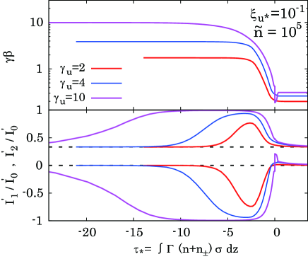
Figure 18: Same as Fig. 5, but for model g2e-1n5 (red), g4e-1n5 (blue) and g10e-1n5 (magenta).

6 Applications

So far, we have focused on the fundamental properties of RRMSs. Here let us consider the applications to GRBs.

Since RRMSs are expected to form in sub-photospheric regions, they should have substantial imprints on the resulting emissions (Bromberg et al., 2011; Levinson, 2012; Keren & Levinson, 2014). As shown in the previous section, when the energy density of the radiation at far upstream is much larger than that of the rest mass energy of the plasma, viz., $\xi_{u*}\gg 1$, thermal spectra with roughly the same peak energy and flux are found at any location in the shock (see top left panel of Fig. 4). This implies that observed spectra produced by a sub-photospheric shock (even if strong) should be nearly thermal when the photosphere is located far below the saturation radius.

On the other hand, significant broadening is expected when the rest mass energy is comparable or larger than that of the radiation at far upstream ($\xi_{u*}\lesssim 1$). This corresponds to shocks that form around or above the saturation radius. To gain some insight into how the radiation will be seen by an observer during the breakout of a RRMS under such conditions, we plot, in Fig. 19, spectra that were averaged over a certain physical interval $\Delta z$, for models g2e-1n5 and g2e-2n5. In addition to the angle integrated spectra that are computed by summing up the contribution of photons in all directions ($4\pi$ steradians), we also display cases where only the photons in a half hemisphere ($2\pi$ steradians) propagating along ($\theta<\pi/2$) and against ($\theta>\pi/2$) the flow are summed up. The former (latter) represents the spectra emitted during the breakout of the reverse (forward) shock that is advancing relativistically in the central engine frame. Hereafter we (loosely) refer to the cases that correspond to photons propagating along and against the flow as reverse and forward shock, respectively. We emphasize that oblique shocks, that are likely to form near the photosphere, are also referred to here as reverse shocks, as their radiation escapes to infinity along the flow. We further point out that the spectra exhibited in Fig. 19 are computed in the rest frame of the shock. In GRBs this frame moves at a high Lorentz factor with respect the observer, and so the observed emission is strongly beamed. Thus, photons moving along the flow may significantly contribute to the observed spectrum also in forward shocks, depending on viewing angle. Our definition of ”forward” and ”reverse” in regards to the integrated spectrum is merely for explication.

As expected, there is a prominent hard component extending above the peak in the case of emission from a reverse shock. It is produced by bulk Comptonization around the RRMS transition layer. The spectrum emitted by a forward shock, on the other hand, lacks such a component (although it is broader than an exponential cutoff), since the high energy photons produced by bulk Comptonization move preferentially along the bulk flow. In both cases, the portion of the spectrum below the peak is softer (broader) than a thermal spectrum. This is due to the moderately bulk Comptonized component in which energy gain by scattering is not so significant, as well as due to the superposition of thermal-like spectra emitted from the upstream and downstream regions. A substantial hardening is also seen at the lowest energies (below the thermal peak of the radiation upstream), since none of the above mentioned broadening effects can play a role.

In comparison with observations, the spectral slopes below and above the peak energy in reverse shocks fall well within the range of detected values. For example, the reverse shock in model g2e-2n5 has low energy and high energy photon indices ($d{\log}I_{\nu}/d{\log}\nu-1$) in the range $-1.5\lesssim\alpha\lesssim-1$ and $-3\lesssim\beta\lesssim-2.5$ for the cases shown in Fig. 19 (middle right panel), which are indeed in good agreement with the observations (e.g., Yu et al., 2016). Similar values are found also for the low energy spectral index $\alpha$ in forward shocks. On the other hand, unlike in reverse shocks, in forward shocks the spectrum above the peak shows a sudden drop off, and is incompatible with a power-law fit. While this is in conflict with Band-like spectra, it is consistent with models that prefer an exponential-cutoff to fit observations, although it could be that those models are misled by an artifact of poor photon statistics at high energies (e.g., Kaneko et al., 2006; Goldstein et al., 2012).

It should be noted, however, that in general the shape of the spectra emitted from a certain fluid shell vary with the width of the shell, or in other words, with spatial interval $\Delta z$ over which they are averaged. As we extend the length of this interval, the contribution from the far downstream and/or upstream regions increases and, therefore, the average spectrum asymptotes to a thermal spectrum. The reason is that the bulk Comptonized component is confined to the vicinity of the shock transition layer by virtue of efficient downscattering of high energy photons by the downstream plasma. This means that in case of a single shock that formed at a distance below the photosphere which is much larger than the width of the shock transition layer, while the signal around the time when the shock reaches photosphere can be highly non-thermal, the time integrated spectrum, that is, the spectrum integrated over the entire duration of burst, would appear quasi-thermal. The broadening at sufficiently low energies might still prevail even then, since its energy exchange rate with electrons is slower than that of the high energy photons. Hence, the low energy broadening has a larger chance to be observed in the overall spectrum.

A more detailed analysis of the properties of photospheric GRB emission requires some knowledge about how shocks are distributed within the outflow, which in turn determines the relative importance of each emission region. This is set by the nature of the central engine as well as by the environment into which the outflow is propagating. Moreover, our calculations are restricted to infinite, steady shocks in planar geometry. While our analysis can describe the shocks at regions well beneath the photosphere, it cannot adequately address the breakout phase during which the photons diffuse out from the system. One must take into account the drastic change in the shock structure during breakout (Beloborodov, 2017; Granot, Nakar, & Levinson, 2017) for a more accurate analysis of the released emission. To that end, dynamical calculations must be performed which is beyond the scope of the present study. Nevertheless, we emphasize that our steady-state simulations confirm that a broad, non-thermal spectrum is an inherent feature of RRMSs which should also be present at the breakout phase. Although more sophisticated computations are necessary for a firm conclusion, we suggest that sub-photospheric shocks may provide a possible explanation for the non-thermal shape in the observed prompt emission spectra of GRBs.

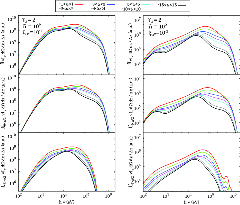
Figure 19: Shock-frame, angle integrated spectra, $\int\nu I_{\nu}d\Omega dz$, averaged over physical distance within a given interval $\Delta\tau*$, for models g2e-1n5 (left) and g2e-2n5 (right). The upper panels show spectra that were integrated over all directions. The middle panels display spectra that were integrated only over photons that propagate toward the downstream ($\theta\leq\pi/2$), and the bottom panels over photons that propagate toward the upstream ($\theta>\pi/2$). The different colors correspond to the special domain over which each spectrum was computed, with red, green, blue, magenta, cyan, gray and black corresponding to $-1<\tau_{*}<1$, $-2<\tau_{*}<2$, $-3<\tau_{*}<3$, $-4<\tau_{*}<4$, $-5<\tau_{*}<5$, $-10<\tau_{*}<10$ and $-15<\tau_{*}<15$, respectively. The scale on the vertical axis is given in an arbitrary units. The absolute value can be determined once either $n_{u}$ or $n_{\gamma,u}$ are specified.

7 Summary and conclusions

We performed Monte-Carlo simulations of relativistic radiation mediated shocks for a broad range of upstream conditions. Since photon generation is not included in the current version of the code our results are applicable only to photon-rich shocks, for which the shock is supported by scattering of back streaming photons that were advected by the upstream flow. To gain insight into the physical processes that shape the structure and spectrum of the shock, the results of the simulations are compared with analytic results whenever possible. Our simulations confirm that the transition from photon rich to photon starved regime occurs when the photon-to-baryon number ratio far upstream satisfies $\tilde{n}\simeq(m_{p}/m_{e})\gamma_{u}$, as expected from an analytic comparison of the advection rate and the photon generation rate by the downstream plasma. At this critical value the downstream temperature approaches the saturation value, roughly $200$ keV, at which it is regulated by vigorous pair creation (Budnik et al., 2010). At sufficiently higher values of $\tilde{n}$ the downstream temperature is much lower, pair loading is significantly reduced, and the shock is supported by the advected photons.

We find that the deceleration of the bulk plasma occurs over a scale of a few pair loaded Thomson depths, with only a weak dependence on upstream conditions; the actual physical scale may be much smaller in cases where vigorous pair production ensues. The shock width increases, but only slightly, when the relative contribution of high energy photons, that are scattered in the KN regime, becomes larger. This is in difference to photon starved shocks in which the shock width is essentially governed by KN effects (Budnik et al., 2010; Granot, Nakar, & Levinson, 2017). We also find that in the photon rich shocks we studied, the temperature of the plasma is determined almost solely by the Compton equilibrium throughout the shock, owing to the high photon-to-baryon number ratio ($\tilde{n}\gg 1$), with the exception of the immediate downstream temperature of the subshock whenever it is present. Apart from these common features, our simulations indicate that the properties of the shock and its emission has a notable dependence on the upstream parameters, $\xi_{u*}$, $\tilde{n}$, and $\gamma_{u}$. Below we summarize our main findings:

• When the energy density of the radiation far upstream largely exceeds the rest mass energy density ($\xi_{u*}\gg 1$), the net increase in the radiation energy across the shock is small. The dominance of the radiation renders the Lorentz factor profile smooth and broad; any attempt of steepening is readily smeared out by the large radiation drag acting upon the plasma. Since the plasma cannot affect much the radiation, the photon distribution is well described by a Wien distribution with a temperature that is equal to that of the local plasma temperature throughout the shock. In our fiducial model with $\tilde{n}=10^{5}$ the large value of $\xi_{u*}$ renders the temperature high enough to induce significant pair production. The resulting population of pairs in this case can be well approximated by the Wien equilibrium.

• The situation changes drastically when $\xi_{u*}\lesssim 1$. In this regime the radiation inside the shock becomes highly anisotropic, and a significant fraction of the upstream bulk energy is converted, via bulk Comptonization of counter streaming photons, to high-energy photons. The consequent photon spectra exhibit a broad, non-thermal component that extends up to an energy of $\sim\gamma_{u}m_{e}c^{2}$. The spectrum inside the shock becomes harder for lower values of $\xi_{u*}$, leading to enhanced pair creation by virtue of the increased number of photons with energies in excess of the pair production threshold. The large pair enrichment in models with high $\gamma_{u}$ and low $\xi_{u*}$ gives rise to a signature of the 511 keV annihilation line in the spectrum.

• It is also found that for sufficiently low values of $\xi_{u*}$ a weak subshock appears, although we were not able to identify its physical origin. Its effect on the overall structure and emission of the shock is negligible, since it only dissipates a small amount of the total bulk kinetic energy. Thus, in practice the presence of the subshock is unimportant for the overall analysis of RRMS, and it is merely of academic interest. The above discussion excludes the cases with $\tilde{n}\simeq m_{p}/m_{e}$ (models g2e-1n3 and g2e-2n3), that delineate a transition between photon rich and photon starved RRMS, and for which a strong subshock was found. As explained above, the presence of a strong subshock in those models is an artifact that stems from the omission of photon production process in our code. Once included, this subshock should become weak (Budnik et al., 2010).

• In order that advected photons will be able to extract the entire upstream bulk energy, the number of advected photons per baryon should exceed $m_{p}/m_{e}$ (i.e., $\tilde{n}>m_{p}/m_{e}$). As stated above, this value marks the transition between photon rich and photon starved shocks. In the photon rich regime the value of $\tilde{n}$ merely determines the downstream temperature, that scales as $T\propto\tilde{n}^{-1}$. As a consequence, the pair production rate depends sensitively on the value of $\tilde{n}$.

• The dependence on the bulk Lorentz factor $\gamma_{u}$ is relatively monotonic compared to the other two parameters. As the Lorentz factor increases, the maximum photon energy attainable through bulk Comptonization increases as $\sim\gamma_{u}m_{e}c^{2}$. Thus, the resulting photon spectra extends to higher energies. The emergence of high energy photons that can diffuse back to larger distances in the upstream region also leads to an increase in the shock width, in the peak temperature in the heating precursor, and in the density of pairs inside the shock.

We also considered the application to GRBs, and have shown that spectra compatible with the observations can be produced within RRMSs. In particular, we demonstrate that the significant spectral broadening occurring in RRMS with $\xi_{u*}<1$ can reproduce the typical Band-like spectrum. This result suggests that RRMS may be responsible, at least in part, for the non-thermal features found in the prompt emission spectra. However, our analysis is limited to infinite, planar shocks, and cannot account for the change in shock structure and emission caused by photon escape during the breakout phase, that may alter the observed spectrum. We intend to carry out detailed analysis of breakout emission in a future work.

Appendix A MONTE-CARLO RADIATION TRANSFER CALCULATION

The Monte-Carlo code used in this study handles transfer of photons in a medium at which Compton scattering, pair production, and pair annihilation takes place. We iteratively perform many calculation runs, in order to find the steady-state shock profile. In each iterative step, the photon transfer is solved under a given profile of number density, $n$ and $n_{\pm}$, temperature, $T$, and velocity, $\beta$ of the plasma as follows: We track the propagation of packets which are ensemble of photons that have identical 4-momentum, $P_{\gamma}^{\mu}=(h\nu/c,(h\nu/c){\bf n})$, where ${\bf n}$ denotes the unit 3-vector along the propagation direction. The photon packets are injected at the inner and outer boundaries which are located at the far upstream and downstream regions, respectively. In addition, pair annihilation processes adds photons into the calculation domain. After the injection, the evolution of the injected packets are computed until they reach the boundaries of the calculation domain or become absorbed via pair production process. During the propagation, they are subject to multiple scatterings by the pair plasma. Between each scattering event, the packet travels in the direction along the 3-vector ${\bf n}$. After the scatterings, their 4-momenta are updated based on the differential cross section of Compton scatterings, and the propagation direction is changed to newly determined ${\bf n}$. Once we finish the calculation, quantities such as total energy-momentum flux and distribution function of photons are evaluated by sampling all of the simulated packets at each grid point,

For each photon packet, distances prior to the scattering and absorption events are determined by drawing the corresponding optical depths, $\delta\tau_{\rm sc}$ and $\delta\tau_{\pm}$. The probability for the selected optical depth to be in the range of [$\delta\tau,\delta\tau+d\tau$] is given by ${\rm exp}(-\delta\tau)d\tau$. From the given optical depths, path lengths to the scattering or absorption events in the laboratory frame (shock rest frame) are determined from the integration of opacity along the ray of photons, which can be expressed as

$$\delta\tau=\int^{l}_{0}{\cal D}^{-1}\alpha^{{}^{\prime}}dl,$$ (34)

where ${\cal D}=[\gamma(1-\beta{\rm cos}\theta)]$ is the Doppler factor. Here $\alpha^{{}^{\prime}}$ denotes the opacity for the corresponding process in the comoving frame of the plasma which can be evaluated from the local physical conditions (see below for detail).

Below, we summarize how the injection of photon packets as well as scattering and absorption processes are treated in our code. Hereafter, we label quantities that are measured in the comoving frame of the bulk plasma with the superscript prime symbol.

A.1 Boundary Conditions

At the boundaries located far upstream and downstream, we assume the photons are isotropic in the comoving frame and have a Wien distribution characterized by the local plasma temperature. Therefore, the photon flux density at the boundary in the laboratory frame is a function of the photon number density and temperature, and can be written as

$$\frac{dN_{\gamma}}{dtd\nu d\Omega dS}={\cal D}^{2}\frac{dN_{\gamma}}{dt^{{}^{\prime}}d\nu^{{}^{\prime}}d\Omega^{{}^{\prime}}dS^{{}^{\prime}}},$$ (35)

where

$$\frac{dN_{\gamma}}{dt^{{}^{\prime}}d\nu^{{}^{\prime}}d\Omega^{{}^{\prime}}dS^{{}^{\prime}}}=\frac{n_{\gamma}}{8\pi}\left(\frac{h}{kT}\right)^{3}\nu^{{}^{\prime}2}{\rm exp}\left(-\frac{h\nu^{{}^{\prime}}}{kT}\right).$$ (36)

Thus, for a given range of solid angles $d\Omega$ and frequencies $d\nu$, $\frac{dN_{\gamma}}{dtd\nu d\Omega dS}(n_{\gamma,{pack}})^{-1}{\rm cos}\theta d\Omega d\nu$ gives the injection rate of the packet number per unit area of the boundary surface, where $n_{\gamma,{\rm pack}}$ is the number of photons contained in a single packet.

A.2 Pair annihilation

The pair annihilation rate per unit volume is evaluated as a function of the pair number density and temperature:

$$\left(\frac{dN_{\pm}}{dtdV}\right)_{\rm ann}=-(n+n_{\pm}/2)(n_{\pm}/2)c\sigma_{T}r_{\pm}(\Theta),$$ (37)

where $\sigma_{T}$ is the Thomson cross section. Here $r_{\pm}$ is an analytical function introduced by Budnik et al. (2010) based on the formula shown in Svensson (1982), which is given by

$$r_{\pm}=\frac{3}{4}\left[1+\frac{2\Theta^{2}}{{\rm ln}(2\eta_{E}\Theta+1.3)}\right]^{-1},$$ (38)

where $\eta_{E}=e^{-\gamma_{E}}\approx 0.56146$ and $\gamma_{E}\approx 0.5772$ is the Euler’s constant. It is noted that the above quantity is Lorentz invariant (i.e., $\frac{dN}{dtdV}=\frac{dN}{dt^{{}^{\prime}}dV^{{}^{\prime}}}$).

As for the energy spectrum of the photons produced via pair annihilation, we use an fitting formula given in Svensson et al. (1996), which approximates the exact emissivity in a wide range of temperatures. By normalizing the given function to be consistent with the Equation (37), it can be written as

$$\left(\frac{dN_{\gamma}}{dtd\nu d\Omega dV}\right)_{\rm ann}={\cal D}\left(\frac{dN_{\gamma}}{dt^{{}^{\prime}}d\nu^{{}^{\prime}}d\Omega^{{}^{\prime}}dV^{{}^{\prime}}}\right)_{\rm ann}$$ (39)

where

$$\left(\frac{dN_{\gamma}}{dt^{{}^{\prime}}d\nu^{{}^{\prime}}d\Omega^{{}^{\prime}}dV^{{}^{\prime}}}\right)_{\rm ann}~{}~{}=~{}~{}~{}~{}~{}~{}~{}~{}~{}~{}~{}~{}~{}~{}~{}~{}~{}~{}~{}~{}~{}~{}~{}~{}~{}~{}~{}~{}~{}~{}~{}~{}~{}~{}~{}~{}~{}~{}~{}~{}~{}~{}~{}~{}~{}~{}~{}~{}~{}~{}~{}~{}~{}~{}$$ (40)

$$\left\{\begin{array}[]{ll}Q_{1}\Theta^{0.5}x_{\nu}^{{}^{\prime}3/2}{\rm exp}\left(-\frac{x_{\nu}^{{}^{\prime}}+x_{\nu}^{{}^{\prime}-1}}{\Theta}\right)\frac{C(x_{\nu}^{{}^{\prime}}\Theta)}{K_{2}(1/\Theta)^{2}}&~{}~{}{\rm for}~{}~{}x_{\nu}^{{}^{\prime}}\Theta\leq 20,\\ Q_{2}x_{\nu}^{{}^{\prime}}({\rm ln}4\eta_{E}x_{\nu}^{{}^{\prime}}\Theta-1){\rm exp}\left(-\frac{x_{\nu}^{{}^{\prime}}}{\Theta}\right)\frac{C(x_{\nu}^{{}^{\prime}}\Theta)}{K_{2}(1/\Theta)^{2}}&~{}~{}{\rm for}~{}~{}x_{\nu}^{{}^{\prime}}\Theta>20.\\ \end{array}\right.$$ (43)

Here $x_{\nu}^{{}^{\prime}}=h\nu^{{}^{\prime}}/(m_{e}c^{2})$, and $K_{2}$ denote the 2nd order modified Bessel function of the second kind. In evaluating the Bessel function, we used the approximate formula

$$K_{2}(1/\Theta)^{2} = 4\Theta^{4}{\rm exp}\left(-\frac{2}{\Theta}\right)$$

$$\times [1+2.0049\Theta^{-1}+1.4774\Theta^{-2}+\pi(2\Theta)^{-3}],$$

which is also given in Svensson et al. (1996). The function $C$ is an analytical function given by

$$C(y)~{}~{}~{}=~{}~{}~{}~{}~{}~{}~{}~{}~{}~{}~{}~{}~{}~{}~{}~{}~{}~{}~{}~{}~{}~{}~{}~{}~{}~{}~{}~{}~{}~{}~{}~{}~{}~{}~{}~{}~{}~{}~{}~{}~{}~{}~{}~{}~{}~{}~{}~{}~{}~{}~{}~{}~{}~{}~{}~{}~{}~{}~{}~{}~{}~{}~{}~{}~{}~{}~{}~{}~{}~{}~{}~{}~{}~{}~{}~{}~{}~{}~{}~{}~{}~{}$$ (45)

$$\left\{\begin{array}[]{ll}\frac{1+6.8515487y+1.4351694y^{2}+0.001779014y^{3}}{1+4.63115589y+1.5253007y^{2}+0.04522338y^{3}}&{\rm for}~{}y\leq 20,\\ 1+2.712y^{-1}-55.6y^{-2}+1039.8y^{-3}-7800y^{-4}&{\rm for}~{}y>20.\\ \end{array}\right.$$ (48)

The normalization factors $Q_{1}$ and $Q_{2}$ are determined from the condition $\int\int\frac{dn_{\gamma}}{dtd\nu d\Omega dV}d\nu d\Omega=-\left(\frac{N_{\pm}}{dtdV}\right)_{\rm ann}$. In our code, for a given range of solid angles $d\Omega$ and frequencies $d\nu$, $\int\int\left(\frac{dN_{\gamma}}{dtd\nu d\Omega dV}\right)_{\rm ann}(n_{\gamma,{pack}})^{-1}d\Omega d\nu$ gives the injection rate of the packet number per unit volume in the calculation domain.

A.3 Compton scatterings

In evaluating the opacity of photons to Compton scattering, we fully take into account the thermal motion of the plasma and Klein-Nishina effects. As a function of the photon frequency, local density of pairs and temperature, it is calculated as

$$\alpha_{\rm sc}^{{}^{\prime}}(\nu^{{}^{\prime}})=\int\int\int F_{\rm sc}({\bf P_{e}},T,\nu^{{}^{\prime}})d{\bf P_{e}}^{3},$$ (49)

where

$$F_{\rm sc}({\bf P_{e}},T,\nu^{{}^{\prime}})=(1-\beta_{e}{\rm cos}{\theta_{e\gamma}})(n+n_{\pm})f_{B}({\bf P_{e}},T)\sigma_{\rm sc}(\nu^{{}^{\prime\prime}}),$$ (50)

and

$$f_{B}(P_{e},T)=\frac{1}{4\pi(m_{e}c)^{3}\Theta K_{2}(1/\Theta)}{\rm exp}\left(-\frac{E_{e}}{kT}\right),$$ (51)

is the Maxwell-J$\ddot{\rm u}$ttner distribution function and

$$\sigma_{\rm sc}(\nu) = \frac{3}{4}\sigma_{T}\biggl{[}\frac{1+x_{\nu}}{x_{\nu}^{3}}\left\{\frac{2x_{\nu}(1+x_{\nu})}{1+2x_{\nu}}-{\rm ln}(1+2x_{\nu})\right\}~{}~{}~{}~{}~{}~{}~{}~{}~{}~{}~{}~{}~{}~{}~{}$$

$$+ \frac{1}{2x_{\nu}}{\rm ln}(1+2x_{\nu})-\frac{1+3x_{\nu}}{(1+2x_{\nu})^{2}}\biggr{]},$$

is the total cross section for Compton scattering. Here $\nu^{{}^{\prime\prime}}$ denotes the frequency in the rest frame of pairs. The quantities ${\bf P_{e}}$, $\beta$ and $\theta_{e\gamma}$ are, respectively, the spatial components of the 4-momentum, the 3-velocity measured in units of the light speed, and the angle between the photon and pair directions measured in the comoving frame, and $P_{e}=|{\bf P_{e}}|$ and $E_{e}=((m_{e}c^{2})^{2}+(P_{e}c)^{2})^{0.5}$.

By plugging in the evaluated opacity in Equation (34), we determine the distance for the photon to propagate before scattering. Once the position of the scattering event is determined, we choose the 4-momentum of a thermal pair that will interact with the photon. The probability for the pair within a range $d{\bf P_{e}}^{3}$ to be drawn is given by $F_{\rm sc}d{\bf P_{e}}^{3}/\alpha_{\rm sc}$. Then we transform the 4-momentum of photons to the rest frame of the chosen electron/positron and determine the 4-momentum after the scattering based on the probability given by the differential cross section of Compton scattering:

$$\frac{d\sigma_{\rm sc}}{d\Omega}=\frac{3}{16\pi}\frac{\nu_{1}^{2}}{\nu^{2}}\left(\frac{\nu}{\nu_{1}}+\frac{\nu_{1}}{\nu}-{\rm sin}^{2}\theta_{\rm sc}\right),$$ (53)

where $\nu_{1}=\nu[1+x_{\nu}(1-{\rm cos}\theta_{\rm sc})]^{-1}$ is the frequency after the scattering and $\theta_{\rm sc}$ is the angle between the propagation directions of the incident and scattered photon. Finally we transform back the 4-momentum of the scattered photon to the laboratory frame and repeat the above cycle until the packet is either absorbed or reaches the surface of the computation boundaries.

A.4 Pair production

For a given 4-momentum of incident photon in the comoving frame, $P_{\gamma}^{{}^{\prime}\mu}=(h\nu^{{}^{\prime}}/c,h\nu^{{}^{\prime}}/c{\bf n^{{}^{\prime}}})$, the opacity for the pair production is calculated as

$$\alpha_{\gamma\gamma}^{{}^{\prime}}(\nu^{{}^{\prime}},{\bf n^{{}^{\prime}}})=\int\int\int(1-{\rm cos}\theta_{\gamma\gamma})f_{\gamma}^{{}^{\prime}}({\bf\tilde{P}}_{\gamma}^{{}^{\prime}})\sigma_{\gamma\gamma}(\nu^{{}^{\prime}},\tilde{\nu}^{{}^{\prime}},\theta_{\gamma\gamma}){\bf\tilde{dP}_{\gamma}}^{3},~{}~{}~{}$$ (54)

where ${\bf\tilde{P}_{\gamma}}=h\tilde{\nu}/c\tilde{{\bf n}}$ and $\theta_{\gamma\gamma}$ denote the spacial component of the target photon 4-momentum and the angle between the propagation directions of the incident and target photons, respectively. Here $f_{\gamma}^{{}^{\prime}}({\bf\tilde{P}}_{\gamma}^{{}^{\prime}})$ is the distribution function of photons in the comoving frame. The cross section for the interaction, taken from Gould & Schréder (1967), is given by

$$\sigma_{\gamma\gamma}(\nu,\tilde{\nu},\theta_{\gamma\gamma})=\frac{3}{16}\sigma_{T}(1-\beta_{\rm cm}^{2})~{}~{}~{}~{}~{}~{}~{}~{}~{}~{}~{}~{}~{}~{}~{}~{}~{}~{}~{}~{}~{}~{}~{}~{}~{}~{}~{}~{}~{}$$

$$\times \biggl{[}(3-\beta_{\rm cm}^{4}){\rm ln}\left(\frac{1+\beta_{\rm cm}}{1-\beta_{\rm cm}}\right)-2\beta_{\rm cm}(2-\beta_{\rm cm}^{2})\biggr{]}~{}~{}{\rm for}~{}~{}\nu\geq\nu_{\rm thr},~{}~{}~{}~{}~{}~{}$$

and $\sigma_{\gamma\gamma}=0$ for $\nu<\nu_{\rm thr}$, where $h\nu_{\rm thr}=2m_{e}c^{2}[h\nu(1-{\rm cos}\theta_{\gamma\gamma})]^{-1}$ is the threshold energy for pair production and $\beta_{\rm cm}=\sqrt{1-2m_{e}^{2}c^{4}/[(1-{\rm cos}\theta_{\gamma\gamma})h^{2}\nu\tilde{\nu}]}$ is the velocity of the pairs in the center of momentum frame. As in the case of Compton scattering, the distance for the photon to propagate before being absorbed via the pair production process is computed by substituting the above opacity in Equation (34).

In our code, the local photon distribution function $f_{\gamma}$ is determined by recording photon packet in each grid point during a single run of the simulation. Since we cannot a-priori know the distribution of the current run before calculation, in each run, we use the photon distribution obtained in the previous step in evaluating the opacity. To ensure the self-consistently of our calculation, we continue the iteration until the difference between the photon distribution evaluated in the current and previous run becomes sufficiently small.

Appendix B CALCULATION OF THE PAIR DENSITY PROFILE

In our code, independent from the energy-momentum conservation, we must determine the pair density profile which satisfy the steady state condition:

$$\gamma\beta c\frac{d(\gamma n_{\pm}\beta)}{dz}=\left(\frac{dN_{\pm}}{dtdV}\right)_{\rm ann}+\left(\frac{dN_{\pm}}{dtdV}\right)_{\rm pr},$$ (56)

where $dz$ denotes the distance element and $(\frac{dN_{\pm}}{dtdV})_{\rm pr}$ is the pair production rate. While the annihilation rate is calculated based on the local quantities as shown in Equation (37), the production rate is evaluated by summing up the number of packets that are absorbed during the propagation in each grid points. During the iteration, pair density profile is modified from the previous iteration step in order to minimize the deviation from the above condition. We continue the iteration until the error becomes sufficiently small.

B.1 Wien equilibrium

When the thermal temperature exceeds $kT\sim 30~{}{\rm KeV}$, copious pairs are produced and can reach the equilibrium state where pair production and annihilation is balanced (Wien equilibrium). In this case, the number density of pairs can be derived as

$$n_{\pm}=n\left(\sqrt{1+\left(\frac{n_{\gamma}}{n}\right)^{2}\left(\frac{K_{2}(\Theta^{-1})}{\Theta^{2}}\right)^{2}}-1\right).$$ (57)

In the limit of $n_{\gamma}\gg n$, it asymptotes to

$$n_{\pm}\approx n_{\gamma}\frac{K_{2}(\Theta^{-1})}{\Theta^{2}}.$$ (58)

If the temperature is non-relativistic, $\Theta\ll 1$, the above equation can be further approximated as

$$n_{\pm}\approx\sqrt{\pi/2}~{}\Theta^{-3/2}{\rm exp}(-\Theta^{-1}).$$ (59)

Appendix C CALCULATION OF THE TEMPERATURE PROFILE

In principle, the plasma temperature profile can be self-consistently obtained by determining the plasma profile for which energy-momentum conservations is satisfied. It is, however, numerically difficult to constrain the temperature profile accurately from the condition $F_{m}={\rm const},F_{e}={\rm const}$ using our iterative method. This stems from the fact that since the contribution of the thermal energy is always much smaller than that of the rest mass energy ($\rho_{pl}\gg e_{pl}$), small numerical errors can lead to large errors in the temperature. On the other hand, the radiation field responds non-linearly to changes in temperature, thereby rendering the calculations unstable and preventing convergence to the steady state solution.

In order to overcome this numerical difficulty, we impose an additional constraint that can be derived from the energy-momentum conservation equations. The equation solves the evolution of internal energy density in comoving frame which is given by

$$\gamma\beta c\frac{de_{pl}}{dz} = \left(\frac{dE^{{}^{\prime}}}{dt^{{}^{\prime}}dV^{{}^{\prime}}}\right)_{\rm sc}+\left(\frac{dE^{{}^{\prime}}}{dt^{{}^{\prime}}dV^{{}^{\prime}}}\right)_{\rm ann}+\left(\frac{dE^{{}^{\prime}}}{dt^{{}^{\prime}}dV^{{}^{\prime}}}\right)_{\rm pr}~{}~{}~{}$$

$$+ (e_{pl}+P_{pl})\gamma\beta c\frac{dn}{dz},$$

where $(\frac{dE^{{}^{\prime}}}{dt^{{}^{\prime}}dV^{{}^{\prime}}})_{\rm sc}$, $(\frac{dE^{{}^{\prime}}}{dt^{{}^{\prime}}dV^{{}^{\prime}}})_{\rm ann}$, and $(\frac{dE^{{}^{\prime}}}{dt^{{}^{\prime}}dV^{{}^{\prime}}})_{\rm pr}$ denote the net heating/cooling rate of the plasma by Compton scattering, pair annihilation, and production, respectively. The last term corresponds to the contribution of adiabatic heating (cooling) due to compression (expansion). While the adiabatic cooling term is evaluated from the local density gradient, $(\frac{dE^{{}^{\prime}}}{dt^{{}^{\prime}}dV^{{}^{\prime}}})_{\rm sc}$, $(\frac{dE^{{}^{\prime}}}{dt^{{}^{\prime}}dV^{{}^{\prime}}})_{\rm ann}$, and $(\frac{dE^{{}^{\prime}}}{dt^{{}^{\prime}}dV^{{}^{\prime}}})_{\rm pr}$, are evaluated by summing up the contributions of scattering, annihilation and production of photon packets in each grid point. By using the above equation, we could successfully obtain an accurate temperature profile.

In our calculations, the temperature is almost solely determined by the condition of Compton equilibrium (net heating and cooling by Compton scattering is balanced, that is., $\left(\frac{dE^{{}^{\prime}}}{dt^{{}^{\prime}}dV^{{}^{\prime}}}\right)_{\rm sc}\sim 0$. This is owning to the fact that the heat capacity of the plasma is extremely small compared to that of the radiation field, since the photon-to-lepton density ratio is large $n_{\gamma}/(n+n_{\pm})\gg 1$. As a result, any small deviation from the equilibrium will inevitably washed out by the numerous photons within a length scale much smaller than the Thomson mean free path $\tau\ll 1$. Notable deviation from the Compton equilibrium temperature is only seen at the immediate downstream region of subshock where instantaneous viscous heating occurs. Note that the downstream of the subshocks in models g2e-1n3 and g2e-2n3 has a large extent ($\tau_{*}\gtrsim 1$) where equilibrium is not established, owing to the vigorous pair enrichment that renders the heat capacity of the plasma comparable to that of the radiation ($n_{\gamma}\sim n_{\pm}$).

References

- Abdo et al. (2009) Abdo A. A. et al., 2009, ApJ, 706, L138
- Ahlgren et al. (2015) Ahlgren B. et al., 2015, MNRAS, 454, L31
- Band et al. (1993) Band D. et al., 1993, ApJ, 413, 281
- Beloborodov (2013) Beloborodov A. M., 2013, ApJ, 764, 157
- Beloborodov (2017) Beloborodov A. M., 2017, ApJ, 838, 125
- Blandford & Payne (1981a) Blandford R. D., Payne D. G., 1981a, MNRAS, 194, 1033
- Blandford & Payne (1981b) Blandford R. D., Payne D. G., 1981b, MNRAS, 194, 1041
- Bromberg et al. (2014) Bromberg O., Granot J., Lyubarsky Y., Piran T., 2014, MNRAS, 443, 1532
- Bromberg et al. (2011) Bromberg O., Mikolitzky Z., Levinson A., 2011, ApJ, 733, 85 (BML11)
- Bromberg & Tchekhovskoy (2016) Bromberg O., Tchekhovskoy A., 2016, MNRAS, 456, 1739
- Budnik et al. (2010) Budnik R. et al., 2010, ApJ, 725, 63
- Colgate (1974) Colgate S. A., 1974, ApJ, 187, 333
- Chevalier (1992) Chevalier R. A., 1992, ApJ, 394, 599
- Drenkhahn & Spruit (2002) Drenkhahn G., Spruit H. C., 2002, A&A, 391, 1141
- Crider et al. (1997) Crider A., Liang E. P., Smith I. A. et al., 1997, ApJL, 479, L39
- Eichler (1994) Eichler D., 1994, ApJS, 90, 877
- Eichler & Levinson (2000) Eichler D., Levinson A., 2000, ApJ, 529, 146
- Ellison et al. (2013) Ellison D. C., Warren D. C., Bykov, A. M., 2013, ApJ, 776, 46
- Ghirlanda et al. (2003) Ghirlanda G., Celotti A., Ghisellini G., 2003, A&A, 406, 879
- Giannios (2012) Giannios D., 2012, MNRAS, 422, 3092
- Globus et al. (2015) Globus N., Allard D., Mochkovitch R., Parizot E., 2015, MNRAS, 451, 751
- Goldstein et al. (2012) Goldstein A., Burgess J. M., Preece R. D., et al., 2012, ApJS, 199, 19
- Gould & Schréder (1967) Gould R. J., Schréder G. P., 1967, Physical Review, 155, 1404
- Granot, Nakar, & Levinson (2017) Granot A., Nakar E., Levinson A., 2017, arXiv, arXiv:1708.05018
- Ito et al. (2013) Ito H. et al., 2013, ApJ, 777, 62
- Ito et al. (2015) Ito H., Matsumoto J., Nagataki S., Warren D. C., Barkov M. V., 2015, ApJ, 814, L29
- Kaneko et al. (2006) Kaneko Y., Preece R. D., Briggs M. S. et al., 2006, ApJS, 166, 298
- Katz et al. (2010) Katz B., Budnik R., Waxman E., 2010, ApJ, 716, 781
- Keren & Levinson (2014) Keren S., Levinson A., 2014, ApJ, 789, 128
- Klein & Chevalier (1978) Klein R. I., Chevalier R. A., 1978, ApJ, 223, L109
- Lazzati (2016) Lazzati D., 2016, ApJ, 829, 76
- Lazzati et al. (2009) Lazzati D., Morsony B., Begelman M., 2009, ApJ, 700, L47
- Levinson (2012) Levinson A., 2012, ApJ, 756, 174
- Levinson & Bromberg (2008) Levinson A., Bromberg O., 2008, Phys. Rev. Lett., 100, 131101
- Levinson & Begelman (2013) Levinson A., Begelman M. C., 2013, ApJ, 764, 148
- Levinson & Globus (2016) Levinson A., Globus N., 2016, MNRAS, 458, 2269
- Lundman et al. (2017) Lundman C., Beloborodov A., Vurm I., 2017, arXiv:1708.02633
- Lyubarskij & Sunyaev (1982) Lyubarsky Y. E., Sunyaev R. A., 1982, Soviet Astron. Lett, 8, 330
- Matzner & McKee (1999) Matzner C. D., McKee C. F., 1999, ApJ, 510, 379,
- McKinney & Uzdensky (2012) McKinney J. C., Uzdensky D. A., 2012, MNRAS, 419, 573
- Mészáros & Waxman (2001) Mészáros P., Waxman E., 2001, Phys. Rev. Lett., 87, 171102
- Morsony et al. (2010) Morsony B., Lazzati D., Begelman M. C., 2010, ApJ, 723, 267
- Murase & Ioka (2013) Murase K., Ioka K., 2013, PhRvL, 111, 121102
- Nakar (2015) Nakar E., 2015, ApJ, 807, 172
- Nakar & Sari (2010) Nakar E., Sari R., 2010, ApJ, 725, 904
- Nakar & Sari (2012) Nakar E., Sari R., 2012, ApJ, 747, 88
- Pai (1966) Pai S. I., 1966, Radiation Gas Dynamics, Springer, New York
- Parsotan & Lazzati (2017) Parsotan T., Lazzati D., 2017, arXiv:1708.01164
- Pe’er et al. (2012) Pe’er A., Zhang B.-B., Ryde F., McGlynn S., Zhang B., Preece R. D., Kouveliotou C., 2012, MNRAS, 420, 468
- Pe’er, Mészáros, & Rees (2006) Pe’er A., Mészáros P., Rees M. J., 2006, ApJ, 642, 995
- Preece et al. (1998) Preece R. D. et al., 1998, ApJL, 506, L23 23
- Rabinak & Waxman (2011) Rabinak I., Waxman E., 2011, ApJ, 728, 63
- Razzaque, Mészáros, & Waxman (2003) Razzaque S., Mészáros P., Waxman E., 2003, PhRvL, 90, 241103
- Riffert (1988) Riffert H., 1988, ApJ, 327, 760
- Ryde et al. (2010) Ryde F. et al., 2010, ApJ, 709, L172
- Ryde & Pe’er (2009) Ryde F., Pe’er A., 2009, ApJ, 702, 1211
- Sapir et al. (2011) Sapir N., Katz, B., Waxman E., 2011, ApJ, 742, 36
- Senno, Murase, & Mészáros (2016) Senno N., Murase K., Mészáros P., 2016, PhRvD, 93, 083003
- Singh, Mizuno, & de Gouveia Dal Pino (2016) Singh C. B., Mizuno Y., de Gouveia Dal Pino E. M., 2016, ApJ, 824, 48
- Sironi et al. (2013) Sironi L., Spitkovsky A., Arons, J., 2013, ApJ, 771, 54
- Skibo et al. (1995) Skibo J. G., Dermer C. D., Ramaty R., McKinley J. M., 1995, ApJ, 446, 86
- Svensson (1982) Svensson R., 1982, ApJ, 258, 321
- Svensson et al. (1996) Svensson R., Larsson S., Poutanen J., 1996, A&AS, 120, 587
- Svirski & Nakar (2014a) Svirski G., Nakar E., 2014a, ApJ, 788, 113
- Svirski & Nakar (2014b) Svirski G., Nakar E., 2014b, ApJL, 788, L14
- Tan, Matzner & McKee (2001) Tan J. C., Matzner C. D., McKee C. F., 2001, ApJ, 551, 946
- Vurm et al. (2013) Vurm I., Lyubarsky Y., Piran T., 2013, ApJ, 764, 143
- Waxman & Katz (2016) Waxman E., Katz B., 2016, arXiv, arXiv:1607.01293
- Weaver (1976) Weaver T. A., 1976, ApJS, 32, 233
- Yu et al. (2016) Yu H. F., Preece R. D., Greiner J. et al., 2016, A&A, 588, A135
- Zel’dovich & Raizer (1967) Zel’dovich Y. B., Raizer Y. P., 1967, Physics of shock waves and high-temperature hydrodynamic phenomena