Near-UV OH Prompt Emission in the Innermost Coma of 103P/Hartley 2

Abstract

The Deep Impact spacecraft fly-by of comet 103P/Hartley 2 occurred on 2010 November 4, one week after perihelion with a closest approach (CA) distance of about 700 km. We used narrowband images obtained by the Medium Resolution Imager (MRI) onboard the spacecraft to study the gas and dust in the innermost coma. We derived an overall dust reddening of 15%/100 nm between 345 and 749 nm and identified a blue enhancement in the dust coma in the sunward direction within 5 km from the nucleus, which we interpret as a localized enrichment in water ice. OH column density maps show an anti-sunward enhancement throughout the encounter except for the highest resolution images, acquired at CA, where a radial jet becomes visible in the innermost coma, extending up to 12 km from the nucleus. The OH distribution in the inner coma is very different from that expected for a fragment species. Instead, it correlates well with the water vapor map derived by the HRI-IR instrument onboard Deep Impact (A’Hearn et al., 2011). Radial profiles of the OH column density and derived water production rates show an excess of OH emission during CA that cannot be explained with pure fluorescence. We attribute this excess to a prompt emission process where photodissociation of H₂O directly produces excited OH*($A^{2}\it{\Sigma}^{+}$) radicals. Our observations provide the first direct imaging of Near-UV prompt emission of OH. We therefore suggest the use of a dedicated filter centered at 318.8 nm to directly trace the water in the coma of comets.

1 Introduction

The hyperactive Jupiter family comet 103P/Hartley 2 was the second target of NASA’s Deep Impact (DI) spacecraft. On 2010 November 4 at 13:59:47 UTC DI passed this small comet at a distance of 694 km from the nucleus with a speed of 12.3 km s^-1 (A’Hearn et al., 2011). Hartley 2 was then at 1.064 au from the Sun and had passed its perihelion one week before. Visible observations of the comet acquired by the spacecraft at closest approach (CA) show the resolved nucleus, with collimated jets from active areas on the surface (Thomas et al., 2013). Spectral observations of the ambient coma show that H₂O gas is enhanced above the central waist, while water ice and dust are spatially correlated with CO₂ jets above the smaller lobe (A’Hearn et al., 2011; Protopapa et al., 2014).

DI observations allowed us to investigate the very innermost regions of the gas coma where the first chemical processes transforming the original parent molecules into fragment species take place. Water is one of the main volatiles sublimating from the nucleus and the most abundant molecule present in the inner gas coma. There, H₂O molecules are destroyed primarily through photodissociation into OH radicals. OH produced in the ground state is consequently excited by solar radiation and decays through the $A^{2}\it{\Sigma}^{+}-X^{2}\it{\Pi}$ transition, producing a strong near-UV (NUV) resonance fluorescence emission (RFE) band at 308.5 nm (Schleicher & A’Hearn, 1982, 1988). Owing to the direct connection between H₂O and OH, this cometary NUV emission has been used for decades as a tracer of the production and distribution of water (A’Hearn et al., 1995).

The Medium Resolution Imager (MRI) (Hampton et al., 2005) onboard DI spacecraft was equipped with a NUV OH filter which allows for the study of OH emission. However, the data from Hartley 2 presented in this paper reveal that some additional emission mechanisms are needed beyond the RFE for interpretation. This will be further discussed in Sec. 6.

The photolysis of water also produces OH*($A^{2}\it{\Sigma}^{+}$) in the first electronically excited state with strongly populated high vibrationally and rotationally excited levels (Carrington, 1964; Harich et al., 2000). This reaction channel, called OH prompt emission (PE), has a smaller but non-negligible branching ratio of 3.6%, compared to 78.4% of OH that is produced into the ground state (for quiet Sun conditions; (Combi et al., 2004, and references therein)). The excited OH* fragments have a short lifetime of about 10^-6 s (Becker & Haaks, 1973) and also decay to the ground state through the same $A^{2}\it{\Sigma}^{+}-X^{2}\it{\Pi}$ transition but with different rotational structure. Due to the different rotational transition, the PE appears broader in wavelength (309–312 nm) than the RFE.

Both the spatial distribution of OH and the rovibrational spectrum can be used to distinguish prompt emission and resonant fluorescence emission.

First, due to their very short radiative lifetime, the OH* radicals do not travel large radial distances with respect to the photodissociating parent molecule, and emit within 0.1 cm from the water molecule they originated from. For comparison the OH RFE lifetime, i.e. the inverse of the fluorescence efficiency, at 1 au varies between 780 and 4500 s, depending on the heliocentric velocity of the comet (Schleicher & A’Hearn, 1988). The morphology of OH PE thus resembles the water distribution rather than the more extended distribution of OH RFE, and PE may exceed RFE in the inner tens of kilometers around the nucleus (Bertaux, 1986; Budzien & Feldman, 1991; Bonev et al., 2004, 2006).

Second, laboratory experiments (Carrington, 1964; Becker & Haaks, 1973) and models (Budzien & Feldman, 1991) indicate that the OH PE spectrum differs from the OH RFE spectrum because different rotational levels are populated.

Thus, very high spatial or spectral resolution is necessary to separate the two emission mechanisms.

The NUV transition is usually followed by additional rotational-vibrational transitions decaying toward lower rotational levels that contribute to an IR band at $\sim$ 3 $\mu$m. OH PE has been measured in both IR and NUV regions but never imaged directly. The 3 $\mu$m PE band has been detected in several ground-based observations of comets (see for example Brooke et al., 1996; Mumma et al., 2001; Gibb et al., 2003; Bonev et al., 2004, 2006). The NUV prompt emission at $308.5$ nm was originally studied by Bertaux (1986) who suggested the presence of a bright spot of $\sim$ 33 km in the inner coma of comet C/1983 H1 (IRAF-Araki-Alcock), and evidence of the PE in the same comet was detected in observations by the International Ultraviolet Explorer (Budzien & Feldman, 1991). Recently A’Hearn et al. (2015) reported the first spectrally resolved detection of NUV OH prompt emission in comet C/1996 B2 (Hyakutake).

In this paper we used narrowband filter observations obtained by MRI instrument on board DI to study the spatial distribution of OH in the innermost coma of Hartley 2, and we investigate the possibility that OH prompt emission is responsible for the observational evidences.

2 Observations and Data Processing

The MRI camera is a 2.1 m focal length Cassegrain telescope, with a 12 cm aperture, a field of view of approximately 35 $\times$ 35 arcminutes, and a per pixel resolution of 2 arcsec (see Hampton et al. 2005 for details). It is equipped with a total of nine filters, five of which are based on the Hale-Bopp narrowband filter set (Farnham et al. 2000). Three narrowband filters are designed to measure different gas species (OH at 309.48 nm and CN at 388.80 nm with bandwidths 6.2 nm, and C₂ at 515.31 nm with bandwidth 11.8 nm), and two other narrowband filters are designed to measure the continuum colors at 345 nm (Violet) and 526 nm (Green); two mediumband filters are designed to measure colors at 750 nm (Red) and 950 nm (IR). The instrument is also equipped with two nearly identical broadband filters (Clear1 and Clear6) sensitive to the whole 200 - 1100 nm wavelength range (Klaasen et al. 2008). The bandpass of the Clear filters includes continuum from light reflected by dust in the coma, as well as emission features from several fragment species, such as OH, CN, and C₂. Since narrowband filters require a relatively long exposure time to get a good signal to noise, during most of the encounter the Clear1 filter was used in order to get an optimal sampling of the comet’s lightcurve. OH, CN and C₂ observations and some color observations were acquired from the day of the perihelion, i.e. 2010 October 28 (DOY 301), through CA occurred on 2010 November 4 (DOY 308), and until 2010 November 16 (DOY 320).

We analyzed a total of 153 OH images ranging from 2010 October 28 to 2010 November 7 (DOY 301-311), acquired from a distance ranging between 10⁶ and 8300 km, with fields of view (FOV) between 10⁴ and 83 km (spatial scales at the comet between 10⁴ and $\sim$ 83 m/pixel). We then focused on the two highest resolution images: image ID 5002027 obtained on DOY 308 about 11 minutes before encounter (E-11 min) from a distance of 8303 km and image ID 5006065 acquired 8.5 minutes after encounter (E+8.5 min) from 8256 km, having both a FOV of about 83 km and a spatial scale of 83 m/pixel. Color images in the Violet, Green and Red filters were acquired close in time to the OH observations (see Table 1), allowing us to study the colors of the continuum and thus perform an accurate subtraction of the continuum light passing through OH bandpass filter.

The MRI dataset used (McLaughlin et al. 2011) was calibrated using the pipeline described in Klaasen et al. (2008, 2013).

As extensively discussed in Klaasen et al. (2013), original images showed residual stripes caused by electrical interference. They implemented an accurate de-striping pipeline which was applied to the data. Despite that, the residual gas data still shows some stripes, probably because of the very low signal to noise. The stripes have a four quadrants pattern in full frame images, due to the 4 amplifiers used to read the CCD. We implemented a further de-striping algorithm in addition to the one implemented in the standard pipeline which takes the average of the first 50 rows from the edge of each quadrant, then fits the stripe pattern with a polynomial function, and finally removes the pattern from the whole quadrant.

Coma structures are usually very faint and hidden by the isotropic component distribution. There are several enhancement techniques that can be used to highlight the anisotropies (see for example Samarasinha & Larson 2011, Farnham 2009). Here, we relied on one of the widely used methods to improve the contrast of the come morphology: the subtraction of the azimuthally averaged radial profile. By subtracting this profile from the original image, anisotropic features of the coma that are otherwise concealed under a brighter isotropic coma, are revealed and a more detailed analysis of the structures and of the spatial distribution is possible (see for example Schleicher & Farnham 2004). To extract radial profiles, images are converted into polar coordinates ($\rho$,$\Theta$) where $\rho$ is the distance in km from the nucleus center, and $\Theta$ is the azimuth angle measured counterclockwise from the vertical line going from the center of the nucleus perpendicularly to the bottom of the image. The profile is fitted with a polynomial function, which is converted into an image and subtracted from the gas image.

3 Continuum Profiles and Colors

The coma brightness in the narrowband gas filters comes from two main components: gas emission lines, and continuum light scattered by the solid materials in the coma such as dust and ice. To isolate the gas emission contribution we need to estimate that of the dust. In visible wavelengths, cometary dust is generally characterized by a featureless spectrum, with a red slope with respect to the solar spectrum (see for example Jewitt & Meech 1986). We used the Violet (345 nm), Green (526 nm) and Red (750 nm) color images acquired together with OH images (see Table 1) to analyze the colors of the coma and subtract the continuum contribution from OH images.

Table 1: OH images acquired at 14:48 UT (E-11 min) and at 14:10 UT (E+8.5 min) on 2010 Nov 4 and color images associated.

image ID	UT	filter	range	FOV
			[km]	[km]
5002027	13:48:25	OH	8303	83
5002029	13:48:55	VIOLET	7883	79
5002034	13:50:06	RED	7185	72
5002035	13:50:10	GREEN	7102	71
5006060	14:09:07	GREEN	6982	70
5006061	14:09:18	RED	7071	71
5006064	14:09:54	VIOLET	7699	77
5006065	14:10:27	OH	8257	83

These images are very close in time to the OH images (less than 2 minutes) and despite the spacecraft movement during CA, the viewing geometry did not change significantly among them.

We rescaled and aligned colors images to the OH image, down to the sub-pixel level. Since the nucleus is resolved for these images, the alignment is done using a projection of a shape model (Thomas et al. 2013) of the nucleus in the image plane. In order to avoid inaccuracies in the pointing, the image alignment is further improved using an iterative cross correlation process at the precision of a quarter of a pixel.

Azimuthally averaged radial profiles of Violet$/$Green, Green$/$Red and Violet$/$Red color maps are shown for image ID 5006065 in Fig.1 with their sunward ($0^{\circ}\leq\Theta\leq 180^{\circ}$) and anti-sunward ($180^{\circ}\leq\Theta\leq 360^{\circ}$) morphology to point out a possible differentiation in the nature of the dust. A zoomed inset shows the region 1-5 km to emphasize the sunward enhancement in all colors. Violet/Red and Violet/Green have been shifted by 0.74 and 0.73 respectively to make them visible in the zoom. Error bars represent the statistical error, i. e. the standard deviation divided by the square root of the total number of pixels used for the average.

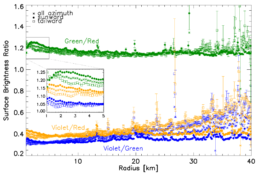
Figure 1: Azimuthally averaged radial profiles of color maps Green/Red, Violet/Red and Violet/Green for image 5006065 (E+8.5 min, FOV 83 km). Sunward (0${}^{\circ}<\Theta<180^{\circ}$) and tailward (180${}^{\circ}<\Theta<360^{\circ}$) profiles are also shown. The inset shows a zoom of the region 1-5 km to emphasize the sunward enhancement in all colors. Violet/Red and Violet/Green profiles have been shifted by 0.74 and 0.73 respectively to make them visible. Error bars represent the statistical error, i. e. the standard deviation divided by the square root of the total number of pixels used to compute the average. Very similar profiles are found for image ID 5002027 (E-11 min, FOV 83 km).

A significant difference is visible between sunward and tailward profiles in all three colors. The sunward profiles show a consistent enhancement in all three colors with respect to tailward profiles within the first 5 km from the nucleus, where the signal to noise is high and the statistical errors are small. This suggests that within 5 km from the nucleus the continuum is bluer in the sunward than in the tailward direction. A possible explanation is an enrichment in water ice. This is strongly supported by the presence of a water ice jet extending to 5 km from the nucleus, observed in the spectral map acquired with the High Resolution Imager (HRI-IR) 7 minutes after encounter (A’Hearn et al. 2011, Protopapa et al. 2014). This color variation, if associated with the water ice jet, suggests that visible colors are sensitive to the presence of water ice in the solid component of the coma.

At larger distances, beyond 20 km from the nucleus, the sunward profiles remain fairly flat, while the tailward profiles show a slight increase. At large radii the statistical errors becomes important because the S/N reduces significantly, in particular for Violet/Red and Violet/Green profiles, where the enhancement is more evident. However, these profiles may suggest a variegation of the solid coma at these distances, getting bluer in the tailward hemisphere.

Only the refractories survive long enough to reach those distances or possibly big icy particles propelled by a rocket effect from sublimation (Kelley et al. 2013). The presence of a larger density of icy particles in the tailward direction may explain the color profiles differentiation. However such variations may be also related to other physical processed happening in the dust coma such as fragmentation.

In order to compare the dust colors with other observations of Hartley 2 we computed the dust reddening maps using the formula by Turner & Smith (1999):

$$R_{1,2}=\frac{{(\frac{I}{F})}_{2}-{(\frac{I}{F})}_{1}}{\lambda_{2}-\lambda_{1}}\frac{20000}{{(\frac{I}{F})}_{1}+{(\frac{I}{F})}_{2}}$$ (1)

where $1$ and $2$ stands for the shorter and longer wavelength respectively among $V$ (Violet), $G$ (Green) and $R$ (Red). Fig. 2 shows the azimuthally averaged radial profiles of the three reddening maps for image ID 5006065. $R_{V,G}$ is about 25%/100 nm close of the nucleus, but decreases to about 12%/100 nm at 40 km. Our results are consistent with the observations by Lara et al. (2011), who showed various reddening profiles in the range 415–693 nm that indicate a decrease of the reddening with distance, as well as variations with direction in the coma. Knight & Schleicher (2013) found reddening lower than $10\%/$100 nm in the wavelength range 345–526 nm within an aperture radius of thousand km.

$R_{G,R}$ is about 9%/100 nm in the vicinity of the nucleus but it increases slightly reaching 13%/100 nm at 40 km. This profile stays much flatter than $R_{V,G}$. The profiles suggest that the spectrum of the dust in the vicinity of the nucleus is similar to the spectrum of the comet’s nucleus (Li et al. 2013) and consistent with the spectral properties of carbonaceous material, which is steeper at bluer wavelengths and flatter at visible wavelengths (Jewitt & Meech 1986). At about 40 km the spectrum of dust coma flattens, and the slopes in the blue and visible regions are consistent with the results found by Knight & Schleicher (2013) for the dust coma at larger distances from the nucleus. This could be interpreted as a change of scattering properties of the solid coma due for example to fragmentation or sublimation of one component (organics). Note that $R_{1,2}$ is a function of wavelength, and that differences in $R$ computed using two different sets of filters (e.g., V-G, G-R) should not necessarily be taken as a change in the spectral slope. We can make general comparisons between the filter sets, and to the literature, but small differences should not be considered significant.

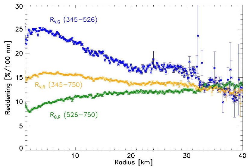
Figure 2: Azimuthally averaged radial profiles of the reddening maps $R_{V,G}$, $R_{G,R}$ and $R_{V,R}$ for image 5006065. Very similar profiles are found for image ID 5002027.

3.1 Continuum removal

To remove the continuum from the OH images IDs 5002027 and 5006065, we assumed that for each pixel in the frame the solid coma has a reflectance spectrum approximated by two straight lines respectively in the wavelenghts ranges 345-526 nm (Violet-Green) and 526-750 nm (Green-Red). We then extrapolated the slope of Violet-Green line to the effective wavelength of the OH filter (309.48 nm) for every pixel. The resulting subtracted continuum is on average 45$\%$ of the total surface brightness, but in the very vicinity of the nucleus it reaches $\sim 95\%$ of the original signal (Fig. 3).

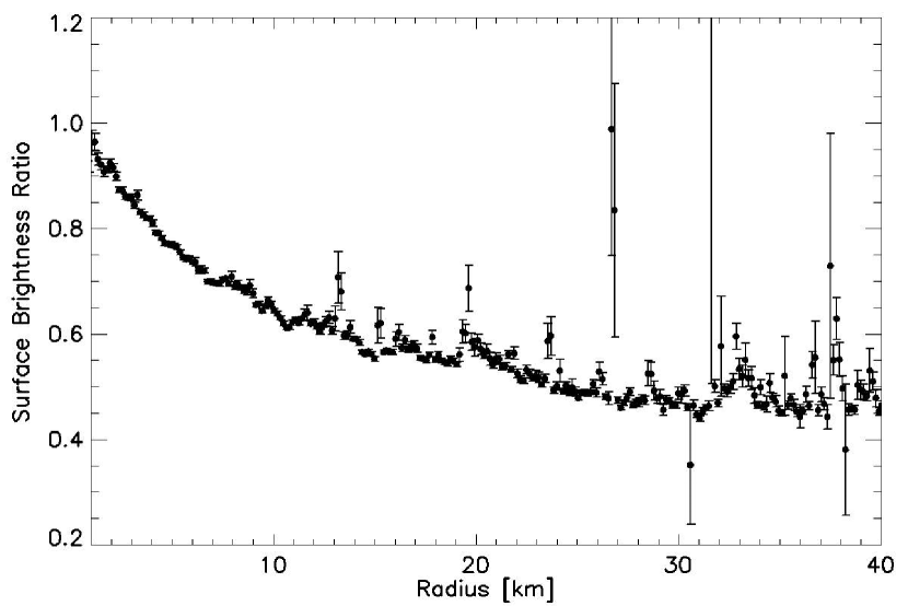
Figure 3: Ratio between the resulting subtracted continuum and the OH original signal azimuthally averaged radial profile for OH image 5006065. Very similar profile is found for image ID 5002027.

For the remaining 151 OH images, the contemporaneous continuum observations were mostly acquired with the Clear1 filter only and no colors or reddening studies can be derived for those images. We therefore used the color information acquired around CA and assumed that the solid coma spectrum remained constant in time during the whole encounter.

For this extrapolation we computed the ratio of the continuum in the OH filter and the signal in each color and Clear1 filter for the images acquired at CA. The azimuthally averaged profiles of all resulting OH/color filter ratios are fairly flat and uniform. Assuming that the dust colors did not change significantly over the considered period, we used the resistant mean of the ratio between the OH profile and each continuum filter profile as the continuum removal factor for that filter. The computed continuum removal factors are: 0.237 for Clear1 filter, 0.615 for Violet filter, 0.201 for Green filter and 0.235 for the Red filter. For comparison, the grey continuum removal factors (Klaasen et al. 2013) computed assuming that the comet has a solar-like spectrum (0.443 for Clear1, 0.668 for Violet, 0.337 for Green and 0.497 for Red) are significantly different, suggesting that the assumption of a solar spectrum, with no reddening, would have significantly overestimated the continuum contribution to the flux measured with the OH filter.

Using the Clear1 observations for the continuum removal is problematic since it is a broad filter (see Hampton et al. 2005), and the flux within its bandpass inevitably contains gas emissions such as CN, C₂, C₃, NH, NH₂. To evaluate this contamination of the Clear1 signal we generated a “synthetic” Clear1 image using the two-straight line spectrum derived from the color images at CA and the Clear1 filter bandpass. The comparison between the observed Clear1 brightness and the synthetic image provided an estimate of the gas contamination of the Clear1 filter. It ranges between 9% in the vicinity of the nucleus to about 12% at the edges of the field of view, slightly increasing with nucleocentric distance. However, using the continuum removal factors computed as described above we indirectly subtract this contribution from Clear1 filter allowing a more precise continuum subtraction with the sole assumption that the colors of the dust remained the same as at CA.

3.2 Uncertainties

MRI-Vis calibration is expected to produce errors of less than 10% (Klaasen et al. 2013) on the total surface brightness. The continuum removal represents the largest uncertainty in measuring the “pure” gas surface brightness.

The original S/N of OH images was typically $\sim$ 5 reaching $\sim$ 13 in the vicinity of the nucleus. Similar values applied to Violet images. While Green observations had generally higher S/N of about 10 with maximum of 22 in the vicinity of the nucleus. Assuming that each image had a calibration error of 10% and propagating the errors for the linear extrapolation, the resulting pure OH gas surface brightness images have an estimated error of about 50%.

4 OH FLUORESCENCE EMISSION

Once the continuum has been removed, the “pure gas” image can be retrieved and converted into OH column densities $N_{OH}$, i.e. the number of molecules along the line of sight in cm^-2, through the formula:

$$N_{OH}=\displaystyle\frac{4\pi\Delta^{2}\Omega d\lambda}{p^{2}g^{\prime}_{OH}}F_{OH}$$ (2)

where $\Delta$ is the distance spacecraft-comet; $\Omega$ is the solid angle of a pixel; $d\lambda$ is the bandwidth; $p$ is the pixel scale of MRI; $F_{OH}$ is the radiance of the pure gas measured in W m${}^{-2}\mu$m^-1 sr^-1 and $g^{\prime}_{OH}$ is the fluorescence efficiency, or $g$-factor, of the OH band as measured through the MRI-OH filter at the heliocentric distance and velocity of Hartley 2.

The $g$-factor describes the efficiency of the molecules in emitting light, and is defined (Chamberlain & Hunten 1987) in cgs units at 1 au for a generic molecule and a single emission line $\lambda$ by:

$$g(\lambda)=\frac{\pi e^{2}}{mc^{2}}\lambda^{2}f_{\lambda}\pi F_{\odot}\tilde{\omega}$$ (3)

where $e$ and $m$ are the charge and mass of the electron and $c$ is the speed of light, $f_{\lambda}$ is the absorption oscillator strength of the molecule, $\pi F_{\odot}$ is the solar flux per unit wavelength at 1 au, $\tilde{\omega}$ is the relative Einstein coefficient for the given line. This has to be scaled for the actual heliocentric distance of the comet at the observation time.

Swings (1941) pointed out that the fluorescence efficiency of some molecules also depends on the heliocentric velocity of the comet. This is because the visible region of the solar spectrum contains strong Fraunhofer absorption lines. The relative motion between the comet and the Sun causes a Doppler shift of the solar spectrum at the comet, affecting the excitation of OH as the lines move in and out of resonance. A change in heliocentric velocity leads to observable differences in the structure of the bands and is particularly important for OH, CN and NH. Schleicher & A’Hearn (1988) computed the fluorescence efficiency for the NUV band of OH for a wide range of heliocentric distances and velocities, and showed that it varies up to a factor of 5.

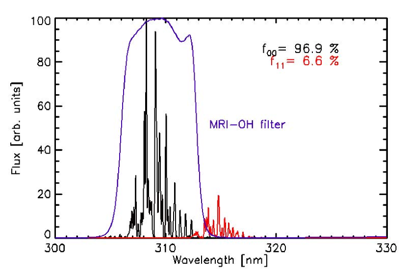
Figure 4: Spectrum of OH fluorescence (0,0) (black) and (1,1) (red) bands obtained using LIFBASE software and the fluorescence levels population distribution (D. Schleicher, priv. comm.) at the heliocentric distance and velocity of Hartley 2. Violet curve shows the MRI-OH bandpass filter weighted for the CCD QE and mirror reflectivity.

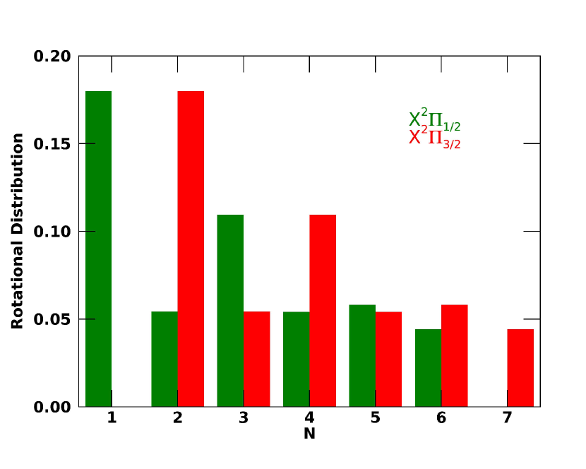
Figure 5: Rotational population distribution of the ground vibrational state for pure fluorescence calculations at the time of EPOXI encounter with Hartley 2. (Schleicher, priv. comm.)

Figure 6: OH column density maps pre-CA. Sun is on the right side.
(a) DOY 304 at 22:38 UTC; FOV 20000 km; spatial scale 39 km pix^-1; linear color scale with range $[10^{12},3\times 10^{13}]$ mol cm^-2
(b) DOY 308 at 09:22 UTC; FOV 500 km; spatial scale 2 km pix^-1; linear color scale with range $[10^{12},7\times 10^{13}]$ mol cm^-2
(c) DOY 308 at 12:16 UTC; FOV 188 km; spatial scale 0.7 km pix^-1; linear color scale with range $[10^{12},7\times 10^{13}]$ mol cm^-2

Figure 7: OH column density maps post-CA. Sun is on the right side.
(a) DOY 308 at 16:31 UTC; FOV 300 km; spatial scale 1.2 km pix^-1; linear color scale with range $[10^{12},7\times 10^{13}]$ mol cm^-2
(b) DOY 308 at 19:31 UTC; FOV 640 km; spatial scale 2.5 km pix^-1; linear color scale with range $[10^{12},7\times 10^{13}]$ mol cm^-2
(c) DOY 310 at 13:46 UTC; FOV 5500 km; spatial scale 21 km pix^-1; linear color scale with range $[10^{12},4\times 10^{13}]$ mol cm^-2

Figure 8: OH column density maps at CA. (a) image ID 5002027; DOY 308 at 13:48 UT; spacecraft distance 8303 km; spatial scale 83 m pix^-1; linear color scale with range $[10^{12},10^{14}]$ mol cm^-2 (b) image ID 5006065; DOY 308 at 14:09 UT; spacecraft distance 8256 km; spatial scale 82.6 m pix^-1. linear color scale with range $[10^{12},10^{14}]$ mol cm^-2. (c) and (d) panels show an enlargement of the (a) and (b) panels respectively in the near-nucleus region to better highlight the nucleus projection and the spatial distribution of OH.

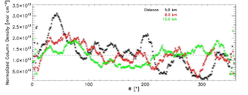
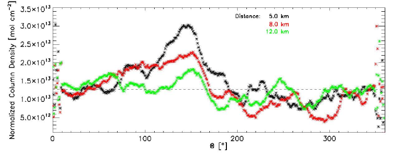
Figure 9: Azimuthal profiles of the OH column density maps in Fig.8: pre-CA image ID 5002027 (top panel) and post-CA image ID 5006065 (bottom panel). Profiles are computed as averages over 1-km width rings centered on the nucleus with radii of 5 (black), 8 (red), and 12 (green) km.

The OH molecules, excited by solar photons to the first electronic state $A^{2}\it{\Sigma}^{+}$, mainly populate the lowest rotational states in the first two vibrational levels $\nu=0$ and $\nu=1$ (Schleicher & A’Hearn 1988). Following the selection rules, OH radicals in these states decay mainly into the vibrational levels $\nu=0$ and $\nu=1$ of the ground electronic state, producing 3 bands: the (0,0) band, centered at 308.5 nm, the (1,1) band, centered at 314.3 nm, and the (1,0) band centered at 283 nm. The (1,0) band is completely outside the MRI-OH bandpass, and to evaluate how much of the (0,0) and (1,1) bands falls within the MRI filter bandpass, we generated a synthetic OH spectrum. For this we use a level population distribution calculated for fluorescence excitation only (D. Schleicher, priv. comm.) at the time of EPOXI encounter with Hartley 2, i.e. for a heliocentric distance ($r_{h}=1.064$ au) and a heliocentric velocity (2.13 km s^-1) and for gas moving 1 km s^-1 towards the Sun. This calculation predicts that the first three vibrational states are populated, with fractions of 75.4%, 23.2% and 1.4% respectively. The ground vibrational state population is in turn distributed in the first 7 rotational levels (Fig. 5).

We then used the LIFBASE software (Luque & Crosley 1999) to generate the resulting emission spectra $S_{00}$ and $S_{11}$.

We weighted this synthetic spectra $S_{00}$ and $S_{11}$ with the MRI CCD quantum efficiency $Q(\lambda)$, mirror reflectivity $R(\lambda)$, and transmission of the OH filter $T(\lambda)$ to calculate the fraction $f_{b}$ of the band flux which is measured by the filter:

$$f_{b}=\frac{\int{S_{b}Q(\lambda)R(\lambda)T(\lambda)}}{\int{Q(\lambda)R(\lambda)T(\lambda)}}$$ (4)

where $b$ can denote either (0,0) or (1,1). The MRI-OH filter has a bandpass of 6.2 nm (Hampton et al. 2005) which includes most of the (0,0) band (96.9$\%$) and a small fraction of the (1,1) band (6.6$\%$) (see Fig. 4).

We used these fractions to calculate the effective fluorescence efficiency $g^{\prime}_{OH}$ as seen through the MRI OH filter as:

$$g^{\prime}_{OH}=\frac{g_{00}(\dot{r}_{h})f_{00}+g_{11}(\dot{r}_{h})f_{11}}{r_{h}^{2}}$$ (5)

where $g_{00}(\dot{r}_{h})$ and $g_{11}(\dot{r}_{h})$ are the $g$-factors of the (0,0) and (1,1) bands respectively (Schleicher & A’Hearn 1988), at the heliocentric distance ($r_{h}$) and velocity ($\dot{r}_{h}$) of Hartley 2.

5 Results: OH in the coma of 103P/Hartley 2

5.1 The Spatial Distribution of OH

We generated OH column density maps for the 153 OH images acquired between the day of the perihelion up to 10 days afterwards using Eq. 2 and the effective $g$-factor in Eq. 5. We selected eight examples of column density maps from the full dataset to show the spatial distribution of OH gas and structures in the coma as representative for three distinct epochs. Fig. 6 shows column densities obtained before CA, Fig. 7 shows three examples acquired after CA, while Fig. 8 shows the OH column density maps of two most resolved images acquired during CA (IDs 502027 and 5006065, see Table 1). In all images the Sun is located on the right side.

We first look at the images pre-CA and post-CA and then we treat differently the two images in Fig. 8 since they have a much smaller scale. A clear anti-sunward enhancement of the OH coma is visible in most of the approach images (DOY 301 – 308). This enhancement has a very sharp fan-like shape in the anti-sunward direction (Fig. 6a). As the spatial resolution increases, a radial jet becomes visible in the sunward direction about 4 hours before CA (see arrow in Fig. 6b) and reaches its maximum brightness at DOY 308 $\sim$ 11:23 UTC. In the following observations, towards the approach to the comet, the OH column density distribution becomes more isotropic with a slight enhancement in the sunward direction (Fig. 6c). After CA, the distribution remains isotropic for very short time (Fig. 7a), after which again an enhancement in the anti-sunward direction becomes visible (Fig. 7b) slightly more toward the left top corner (Fig. 7c) with respect to the pre-CA images.

Although Hartley 2 has been studied in great detail from the ground and from space, its rotational state is not yet fully understood due to its very complex rotation. (Belton et al. 2013, Knight et al. 2015). Therefore, it is not straightforward to establish if the observed spatial variations in OH distribution are due to diurnal or long-period variations. Most likely they are the result of a combination of factors such as the single and triple peaked light-curve variations with a period near 54–55 hr and the change in observing geometry between pre-CA and post-CA.

Fig. 8 allows us to analyze the OH spatial distribution closest to the nucleus, revealing structures at much smaller scales. In both images the Sun is located on the right side while the different orientation of the nucleus is due to the movement of the spacecraft. The geometrical effect of the spacecraft motion is that images after CA are roughly upside down compared to those before the CA. A radial structure coming from the central waist of the nucleus is visible in both images, but more evident in Fig. 8b.

In order to measure reliably the opening angle and the angular extent of this feature we plot the azimuthal profiles (Fig. 9) of the OH column density averaged over rings of 1 km width, centered on the nucleus, respectively with radii of 5, 8, and 12 km. The azimuth angle $\Theta$ is measured counterclockwise from the vertical line going from the center of the nucleus perpendicularly to the bottom of the image. The profiles have been normalized such that the average value of each profile corresponds to the average of the profile at 5 km, represented by the dashed line in the plots. The original average values did not differ anyway by more than a factor 2. Before CA (Fig. 8a) the OH jet has a peak around $\Theta\sim 40^{\circ}$, while after CA (Fig. 8b) it is directed towards $\Theta\sim 140^{\circ}$–150^∘, which is compatible with the geometrical change between the two frames, indicating the persistence of the jet. The OH radial structure has an opening angle of about 30^∘ before CA which becomes broader after CA to about $40^{\circ}$ and extends up to about 12 km from the nucleus’ surface. After CA it seems to have a second component blending down to the right of the central plume giving rise to a “fountain-like” structure.

Figure 10: (a) HRI-IR water vapor spectral map acquired 7 minutes after CA scaled, rotated and shifted to be superimposed on MRI-OH ID 5006065 column density map in Fig 8b. (b) An enlargment of panel a within the near-nucleus region.

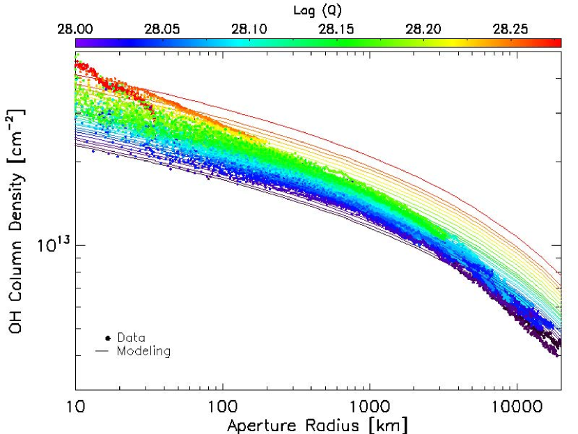
Figure 11: Radial profiles of OH column density azimuthally averaged for all 153 images acquired in the period DOY 301-311. Solid lines show the Haser-based model profiles for various production rates values according to the colorbar. The observed data points have the color of the best-fitting model profile.

Figure 12: OH column density profiles sunward side (a) and anti-sunward (b) for a total of 12 images acquired between 10 min and 14 hours after CA. The colors of the data points indicate the acquisition time according to the colorbar. For each observed profile the best-fitting model profile has been plot with the same color of the observed profile. The corresponding production rate values are not indicated since the aim of the plot is to show the deviation of the observed profiles with respect to the models in the sunward direction as opposed to the very good accordance obtained for the anti-sunward profiles.

The observed spatial distribution differs from what we would expect for fragment species. Fluorescent OH transitions have lifetime of about 4000 s at the heliocentric distance and velocity of Hartley 2 at the moment of observation. Such long lifetime would dimish the effects of potential spatial asymmetries in the distribution of the parent water molecule on the distribution of the fluorescent emission from OH. However, the observed distribution resembles more a parent-like distribution. We compared the OH structure visible in Fig. 8b with the water vapor spectral map obtained on DOY 308 14:07 UTC (about 7 minutes after CA) by the HRI Infrared instrument (HRI-IR) on board DI (A’Hearn et al. 2011, Protopapa et al. 2014, Fig. 11A). The HRI-IR map has a spatial resolution of 55 m pix^-1 and covers a region of about 5 km, much smaller than MRI FOV (70 km). It has been rescaled, rotated and shifted to the MRI image, so that the nucleus was superimposed in the two frames (Fig. 10). The HRI-IR image shows a strong water vapor plume coming from the central waist of the nucleus. The OH structures in the MRI are clearly a continuation of the water vapor plume coming from the comet’s waist seen by HRI-IR. The strong spatial correlation between non-isotropic appearances of OH and H₂O suggests that a non-RFE component contributes to the total OH flux. The excited OH* fragments, having a very short radiative lifetime of about 10^-6 s, instantly decay preserving the spatial distribution of the parent molecule.

5.2 Radial Column Density Profiles

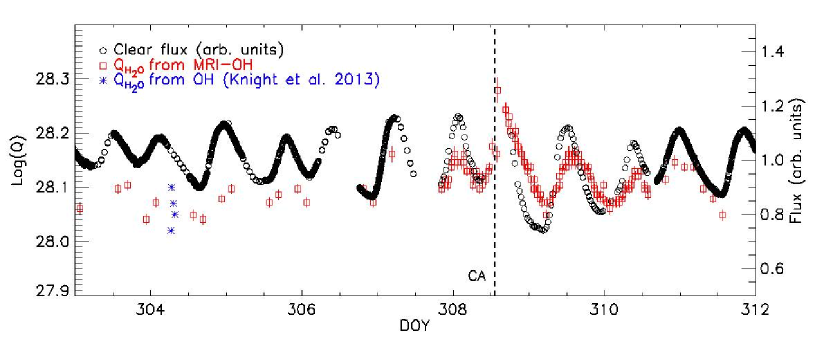
Figure 13: Temporal Variation of water production rate derived from MRI-OH observations using a two-generation Haser model (red squares), compared with Clear1 visible light curve (arb. scaled) within an aperture of 14 pixels (black circles) (Williams et al. 2012). Groundbased water production rates by Knight & Schleicher (2013) are also shown for comparison.

For each image of the dataset we extracted an azimuthally averaged radial column density profile. The full dataset provides a good coverage of the coma between 10 km and a few thousand kilometers from the surface. Given the anti-sunward enhancement observed in the OH spatial distribution pre- and post-CA (Fig. 6 and 7) and the strong sunward radial jet observed at CA (Fig. 8), we separately studied sunward and anti-sunward profiles inside 1000 km from the nucleus in 12 images acquired between 10 minutes and 14 hours after CA.

The 153 OH column density profiles are shown in Fig. 11. They are overall consistent and form a regular trend without significant discontinuity. The sunward profiles (Fig. 12a), acquired between 0 and 14 hours from CA, show a rapid change both in absolute value and in their shape. The observed profiles become increasingly steeper approaching CA and the OH column density at 10 km from the nucleus doubles in about eight hours compared to the column density before CA. The anti-sunward profiles (Fig. 12b) remain flatter than the sunward profiles.

We compare the azimuthally averaged column density profiles with modeled profiles. The Haser (1957) model describes the distribution of fragment species. It assumes a spherically symmetric source of uniformly outflowing parent molecules that photodissociate with an exponential lifetime to create fragment species. In the vectorial model (Festou 1981) the daughter molecule has an excess velocity from the photodissociation of the parent. As a consequence the daughter does not have the same outflow velocity of the parent but may have an isotropic distribution around the parent molecule.

Despite the limitations of the standard Haser model (see, e.g., Crifo et al. 2004) it is a commonly used model for a direct comparison of different observations owing to its simplicity. Moreover, in the inner coma collisions enforce a radially outward flow (Woodney et al. 2002) thus making the Haser model still useful for spatial radial profile fits in these regions. Since a more detailed and complex numerical model, such as the Monte Carlo and the updated DSMC calculations (see, e.g., Combi & Smyth 1988, Tenishev et al. 2008), is out of the scope of this paper and a simple relative comparison is sufficient here, we decided to proceed with a modified two-generation Haser model. We used the transformation equations in Combi et al. (2004) that relate a realistic spatial profile obtained with the vectorial model to the equivalent Haser scalelengths and lifetime. We adopted the typical values for gas velocity of $v=1$ km s^-1, lifetime of water $\tau_{H_{2}O}=0.96\times 10^{5}$ s and lifetime of OH $\tau_{OH}=1.5\times 10^{5}$ s (Combi et al. 2004). We ran computations for a series of production rates ranging between $10^{28}$ mol s^-1 and $2\times 10^{28}$ mol s^-1 with incremental steps of $0.02-0.05\times 10^{28}$ mol s^-1. The modeled number densities are then integrated along the line of sight and used in comparison with the observed column densities profiles. The model with the smallest residuals represents the best fit among the computed curves. The general agreement found between the observed and the modeled profiles – except for the very inner coma – justifies our approach.

The modeled column density profiles are shown as solid lines in Fig. 11 and 12. They adequately fit most of the column density profiles apart from the very innermost regions (inside 20 km) observed at close distances in the sunward direction, where the data show higher and steeper column densities with respect to the model. The measured antisunward OH profiles show an increase in the OH column density as we get close to the CA that is much more in accordance with the modeled column density profiles. A possible explanation for this dichotomy is the presence of two OH emission components: the first a tailward component, stable in time and changing with the rotation of the nucleus, and compatible with the predicted fragment species distribution of OH; and a second component, mainly sunward, deviating from the model prediction and requiring a much higher number of OH molecules, and likely correlated with the water gas plume observed in HRI-IR maps (A’Hearn et al. 2011). The OH column density in the sunward direction can be due to a different emission process in addition to fluorescence. We will discuss this further in the next section.

5.3 Production Rates

The adopted model is based on the assumption that OH is produced solely by photodissociation of H₂O, and that OH emission is driven by RFE. The best fit of each column density profile is then used, under these circumstances, to derive the water production rate.

The temporal variation of the water production rate is shown with red empty squares in Fig. 13. We compare this with the visible light curve observed through the Clear1 filter within 14 pixels aperture (black filled circles) (Williams et al. 2012) to investigate the correlation between gas and dust activity. Ground-based water production rates by Knight & Schleicher (2013) are also overplotted for comparison. The agreement between the dust and gas light curves, in particular outside the CA peak, suggests that the OH emission correlates well with the dust content of the coma and the rotation of the comet, despite the different escape speed of the two components. The latter is likely responsible for the small shift between the curves. The amplitude of the water production rate is smaller than the amplitude of dust light curve in this relative scale, except for the peak at CA, which shows a much higher water production rate with respect to all other peaks. Since no physical relevant changes are expected in the comet’s activity corresponding to the approach of the spacecraft, apart for an increased spatial resolution, the increased amplitude of the CA peak is further evidence that a mechanism other than fluorescence drives part of the OH emission.

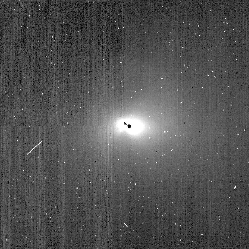
Figure 14: Resulting continuum image subtracted from OH image ID 5006065. A linear stretch of the square root histogram of the image is used for visualization.

6 Discussion

6.1 Emission Processes

There are two clear indications that OH fluorescence is not the sole mechanism producing the observed emissions through the MRI-OH filter. First, the data show a strong jet in the innermost coma of Hartley 2, extending up to 12 km from the nucleus (see Fig. 8), with a significant correlation with the water gas distribution observed through HRI-IR (see Fig. 10). Second, the column density profiles deviate from an Haser-based model only in the very vicinity of the nucleus in the sunward direction, resulting in an excess peak in the derived water production rate at CA that is not expected from an increase in spatial resolution only (see Fig. 12a).

The jet visible in OH at CA is not present in the continuum image (Fig. 14), which has a completely different morphology with a more circular distribution around the two lobes of the comet, in agreement with the dust distribution observed by HRI-IR and HRI-VIS (Protopapa et al. 2014). We therefore rule out that the OH feature can be attributed to a residual dust jet.

We investigated the possibility that this emission is produced by a species other than OH. The only feature at these wavelength which may contribute to the observed emission is the B${}^{3}\it{\Sigma}_{u}-$X${}^{3}\it{\Sigma}_{g}$ band of S₂ molecule. S₂ has a short lifetime of a few hundreds seconds at 1 au, so it is present only very close to the nucleus.

The S₂ fluorescence rates are approximately 4$\times 10^{-4}$ ph s^-1 mol^-1 (A’Hearn et al. 1983), comparable to the OH fluorescence efficiency at Hartley 2 ($2.4\times 10^{-4}$ ph s^-1 mol^-1). S₂ has been observed in a small number of comets and abundances with respect to water are of order 0.001–0.1% (A’Hearn et al. 1983, de Almeida & Singh 1986, Kim et al. 1990, Weaver et al. 1996, Laffont et al. 1998, Bockelée-Morvan et al. 2004). Because the number of OH molecules is at least 100 times larger than the number of S₂ molecules we expect its contribution to the observed emission to be very small.

Another possibility is that excess OH comes either directly from the nucleus, or from slowly moving grains in the coma, in a similar way that CN seems to have these contributions (Bockelee-Morvan & Crovisier 1985, Fray et al. 2005). If the “fountain-like” structure observed in the post-CA (Fig. 8b) is real, its presence would support the hypothesis that OH is coming from slowly moving grains that are fountaining out over a significant portion of the rotation arc. However, this scenario would not explain the very good correlation observed in the inner coma between OH and water gas (Fig. 10). The direct emission from excited OH* molecules is instead a plausible candidate to explain our observations. The two most likely processes to produce excited OH* from H₂O in the coma are dissociative electron impact excitation (DEIE) and emissive photodissociation, also called prompt emission (PE), respectively:

$$\textnormal{DEIE}: \hskip 14.22636ptH_{2}O+e\to OH^{*}+H$$ (6)

$$\textnormal{PE}: \hskip 14.22636ptH_{2}O+h\nu\to OH^{*}+H$$ (7)

The production of excited water group fragments (O*, OH*, OH*⁺) by electron impact has been observed in the inner coma of comet 67P/Churyumov-Gerasimenko by the Alice and OSIRIS instruments on board the Rosetta spacecraft (Feldman et al. 2015, Bodewits et al. 2016). Like MRI, the OSIRIS instrument was equipped with narrowband filters to image the gas and dust in the coma. Similar to the results described here, it observed an excess of emission in the OH filter (and in its OI, NH, and CN filters), and the morphology of the emission indicated a process that directly produced OH in the $A^{2}\it{\Sigma}^{+}$ state. The surface brightness in the inner 100 km of the coma was orders of magnitude larger than could be explained by photo processes. As the comet got closer to the Sun and its production rates exceeded several time 10²⁷ molecules s^-1, emission levels dropped to ’normal’ levels. Bodewits et al. (2016) attributed this to decreasing electron temperatures; below 10 eV electron impact collisions lead to ro-vibrational excitation of H₂O molecules rather than to dissociative or ionizing reactions.

Both DEIE and PE produce OH emission that falls within the passband of MRI-OH filter (next section) and the Deep Impact spacecraft was not equipped with any plasma instruments that would allow us to distinguish between the two emission processes. However, the EPOXI observations of 103P/Hartley 2 were acquired at 1.064 au, when the comet had a water production rate of 10²⁸ molecules s^-1. The physical environment in the inner coma then was comparable to that of 67P/Churyumov-Gerasimenko during perihelion when photo processes rather than electron impact drove the emission. That environment is likely also analogue to the inner coma of comet Hyakutake, for which A’Hearn et al. (2015) used high-resolution spectra to distinguish PE from DEIE and PE. We therefore find the prompt emission scenario more likely than the electron impact scenario and will quantitatively test this hypothesis in the next section.

6.2 Prompt Emission Scenario

The fluorescence mechanism mainly populates the first 5 rotational levels of OH*$(A^{2}\it{\Sigma}^{+}$). (Schleicher & A’Hearn 1988). The direct population of OH*($A^{2}\it{\Sigma}^{+}$) by photodissociation of water has been studied by many authors. Carrington (1964) found that the rotational levels from 18 to 23 are the most populated states, supported by later studies by Yamashita (1975) and Mordaunt et al. (1994). Harich et al. (2000) also found that highly rotationally excited OH(A) products are dominant. This result has been also recently confirmed by the observation of OH PE lines in the spectrum of comet Hyakutake (A’Hearn et al. 2015).

The excited OH*$(A^{2}\it{\Sigma}^{+}$) molecules directly decay emitting at slightly higher wavelengths than fluorescence and with a different intensity in the NUV. We produced synthetic OH spectra for both prompt emission and fluorescence emission using the software LIFBASE (Luque & Crosley 1999), assuming population distributions for PE from Carrington (1964) and Schleicher’s (priv. comm.) for RFE. The resulting synthetic spectra are shown in Fig. 15 together with the MRI-OH bandpass. The PE spectrum is broader and centered at higher wavelength, however a non negligible fraction, $f_{PE}$, passes through the MRI-OH filter. Using Eq. 4 we calculated this fraction by weighting the PE spectrum with the MRI-OH filter bandpass, mirror reflectivity and CCD quantum efficiency, and find that a fraction of $f_{PE}=38.75\%$ of all PE emission is sampled by the MRI and its OH narrowband filter. For comparison, the Rosetta/OSIRIS OH filter (Keller et al. 2007) has a slightly narrower bandpass (4 nm) and blocks longer wavelengths than the MRI filter, making it less sensitive to OH PE.

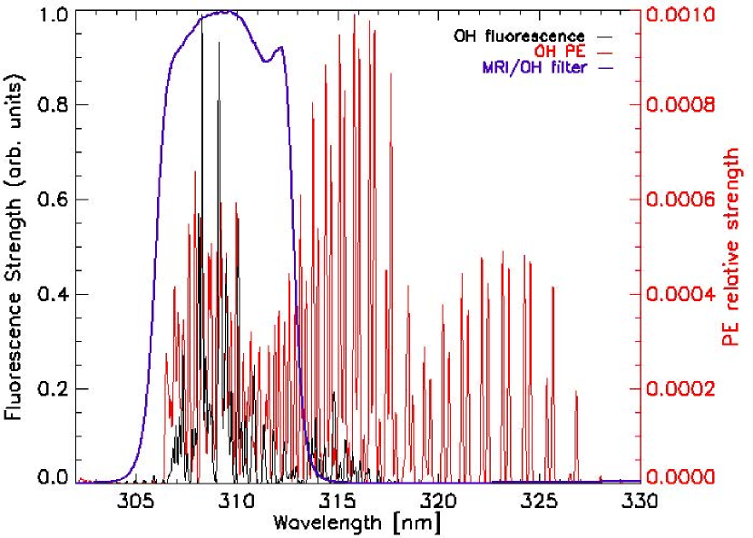
Figure 15: OH Fluorescence (black) and prompt (red) emission spectral distributions obtained with LIFBASE software and population distribution by Schleicher (priv. comm.) and Carrington (1964) respectively. Violet curve shows the MRI-OH bandpass filter weighted for the CCD QE and mirror reflectivity.

The theoretical contribution $S_{PE}/S_{FE}$ of the two mechanisms, as function of the projected distance $\rho$ from the comet’s nucleus in the sky plane, can be calculated by:

$$\frac{S_{PE}}{S_{FE}}(\rho)=\frac{N_{\text{H}_{2}\text{O}}(\rho)}{N_{\text{OH}}(\rho)}\frac{DBr(\text{OH}^{*}(A^{2}\it{\Sigma}^{+}))f_{PE}}{g^{\prime}_{\text{OH}}}$$ (8)

where $N_{\text{H}_{2}\text{O}}(\rho)$ and $N_{\text{OH}}(\rho)$ are the column densities of H₂O molecules and OH molecules at the projected distance from the nucleus $\rho$; $D$ is the photodestruction rate of water molecules, i.e. the total number of water molecules which actually photodissociate per second; $Br(\text{OH}^{*}(A^{2}\it{\Sigma}^{+}))$ is the branching ratio for the production of OH*$(A^{2}\it{\Sigma}^{+})$, i.e. the fraction of OH molecules left in the excited $A^{2}\it{\Sigma}^{+}$ electronic state relative to the total number of OH radicals produced by photodissociation; $g^{\prime}_{\text{OH}}$ is the effective fluorescence efficiency described in Sec. 4, and $f_{PE}$ is the fraction of the PE spectrum visible through the MRI-OH filter.

Table 2: Lifetime, photodestruction rate of H₂O and branching ratios for OH*($A^{2}\it{\Sigma}^{+}$) (Combi et al. 2004)

	$\tau_{\text{H}_{2}\text{O}}$	$D$	$Br(\text{OH}^{*})$
	[s]	[mol s-1]	[$\%$]
Quiet Sun	9.6E4	1.04E-5	3.6
Active Sun	7.1E4	1.41E-5	4.1

The ratio $\frac{N_{\text{H}_{2}\text{O}}}{N_{\text{OH}}}(\rho)$ in Eq. 8 has been estimated using the two-generation Haser model adopted in the previous section. Given the low activity of the Sun at the time of the encounter we used the quiet Sun values from Combi et al. (2004) summarized in Tab. 2. The ratio $\frac{N_{\text{H}_{2}\text{O}}}{N_{\text{OH}}}(\rho)$ is independent of the water production rate value and decreases exponentially with the projected distance from the nucleus. The photodestruction rate and the PE branching ratio depend mainly on the solar activity.

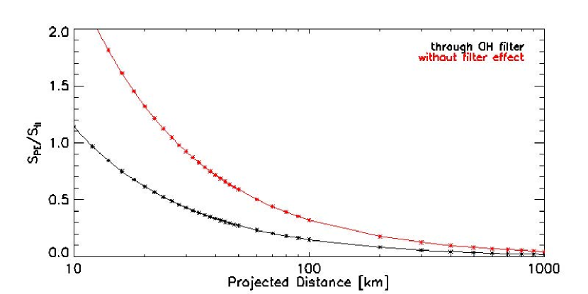
Figure 16: Relative strength of OH prompt emission to fluorescence emission as function of the projected distance from the nucleus modeled using a two-generation Haser model, as seen through MRI-OH filter (black line) and without the effect of the filter (red line).

The total theoretical ratio $S_{PE}/S_{FE}$ in Eq. 8 as seen through the MRI OH narrowband filter, and the same ratio without the effect of the filter, have been computed for $\rho$ between 10 and 1000 km and are shown in Fig. 16. Close to the nucleus the PE is as efficient as RFE but outside $\sim$20 km fluorescence becomes the dominant emission mechanism. This analysis suggests that a non negligible fraction of the OH flux in the innermost coma may be actually attributed to OH prompt emission.

If the dominant emission mechanism is indeed PE, we would overestimate the OH column densities derived assuming fluorescence efficiencies. To retrieve pure fluorescence column densities, we used the total strength ratio $S_{PE}/S_{FE}$ to subtract the expected PE fraction from the measured OH column density. The total theoretic fraction results higher than the value which is needed for the profiles to agree with the models. If we subtract 40% of the theoretical PE computed, the modified column density profiles and the models agree much better (Fig. 17), even in the innermost coma. The models are still not an adequate fit to the residual pure fluorescence column density profiles, but this can be attributed to the limitations of the Haser-based model for the inner coma.

The water production rate variation curve has been also corrected assuming the same adjusted prompt emission factor (Fig. 18). The strong CA peak is remarkably reduced if compared with Fig. 13 and is now more in line with the periodicity variation.

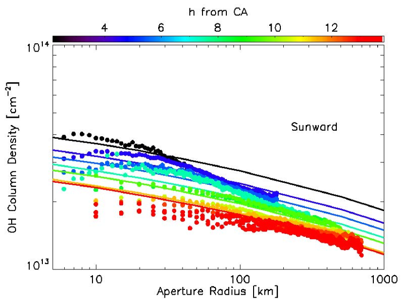
Figure 17: Sunward column densities profiles as in Fig. 12 but corrected for 40% of the theoretical estimated prompt emission.

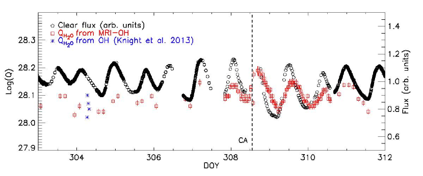
Figure 18: Water production rate (red squares) corrected for 40% of the theoretical estimated prompt emission compared with Clear filter light curve (arb. scaled) within aperture of 14 pixels (black circles) (Williams et al. 2012). Ground based water production rates by Knight & Schleicher (2013) are plotted for comparison.

This suggests that the PE mechanism is able to explain the data within a factor two, which is acceptable given the large uncertainties in the numerical parameters used in the modeling and considering the several physical processes that we did not include in the calculations. Photodestruction rates and branching ratios may vary significantly due to the solar activity and they are affected by large uncertainties in calculated reaction cross sections. The assumed velocity and lifetimes of the fragments might vary by several factors in this very complex region of the coma with respect to the typical assumed values. The fraction $f_{PE}$ strongly depends on the assumed rotational and vibrational population distribution, which has its intrinsic uncertainties (see for example A’Hearn et al. (2015)). The optical depth effect is not included in the calculations because the PE lines are optically thin but the inner coma is opaque to solar Ly_α. Moreover, collisions in the innermost coma could in principle de-excite a fraction of OH* molecules, thus reducing the effective PE observed. Given the very short lifetime (10^-6 s) of these fragments (Becker & Haaks 1973, A’Hearn et al. 2015), very high molecular densities would be required for collisions to significantly de-excite the OH* radicals. However, given the importance of electron impacts observed by Rosetta at comet 67P/Churyumov-Gerasimenko (Feldman et al. 2015, Bodewits et al. 2016), we carried out a rough estimate of the collisional rate of OH* molecules with electrons and neutrals (mainly water molecules) in the inner coma.

6.3 Collisional Quenching

The collisional rate, $R_{c}$ is given by:

$$R_{c}=\sigma_{c}n(\rho)v$$ (9)

where $\sigma_{c}$ is the collisional cross section, $n(\rho)$ is the density of the collisional partner at cometocentric distance $\rho$, and $v$ is the typical relative speed. Collisions with electrons are more efficient in de-exciting the OH radicals than collisions with neutrals because the collisional cross section of electrons and OH* is about $10^{-10}$ cm² (Schleicher & A’Hearn 1988), while the total cross section of impacts by neutrals is about $1-5\times 10^{-14}$ cm² (Bockelée-Morvan et al. 2004).

The Langmuir Probe (LAP) and Mutual Impedance Probe (MIP) on Rosetta measured the electron number density at 10 km from the comet 67P/Churyumov-Gerasimenko when it was at 2.3 AU from the Sun (Edberg et al. 2015). If we assume that the number density scales linearly with the water production rate and the photoionization rate, and thus the square of the heliocentric distance (Bodewits et al. 2016), the electron number density at Hartley 2 at about 50 km from the nucleus would be about 10⁴ cm^-3. Bhardwaj et al. (1996) developed models of electron density profiles based on observations of comet Halley, whose production rate was 5-10 times higher than Hartley 2, finding electron density of 10⁵ cm^-3 at 50 km from the nucleus. (see also Biver et al. 1999). We conservatively assumed as upper limit the electron density profile modeled by Bhardwaj et al. (1996) for higher activity conditions to calculate the collisional rate.

The number density of water molecules, certainly the most abundant species in the inner coma, is about $3.7\times 10^{8}$ cm^-3, calculated using the two-generation Haser model assuming a production rate of $1.17\times 10^{28}$ mol s^-1, the average of the water production rate derived from MRI-OH observations.

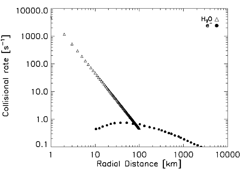
Figure 19: Collision rate of OH* molecules with electrons (filled circles) and water molecules (open triangles) as function of the projected distance from the comet based on Bhardwaj et al. (1996) electron density and water molecules density derived using an Haser-based model and a production rate of $1.17\times 10^{28}$ mol s^-1, the average of the water production rate derived from MRI-OH observations.

The collisional rates of OH radicals with both electrons, and water molecules are shown in Fig. 19 as a function of the radial distance from the comet. Even when we assume the upper limit for the electron density we find that the collisions with neutrals are dominant in the innermost regions up to about 100 km since the local ratio n${}_{\text{H}_{2}\text{O}}$/n${}_{e^{-}}$ is very large (see also Bockelée-Morvan et al. 2004).

At 10 km from the nucleus the collisional lifetime $\tau_{c}=1/R_{c}$ of OH* is thus about 0.4 s, much longer than the radiative lifetime of OH* expected to be about 10^-6 s (Becker & Haaks 1973). Therefore collisional quenching does not significantly de-excite the OH* radicals.

7 Summary

The EPOXI mission allowed us to investigate the innermost coma of 103P/Hartley 2, with high spatial resolution, revealing regions and processes usually unobservable with ground based observations.

We analyzed the dust colors using the color filters mounted on the MRI camera and found that the dust coma in the first 5 km from the nucleus is bluer in the sunward direction than in the tailward direction. We attributed this to an enrichment in water ice in the sunward coma, as supported by HRI-IR spectral maps (A’Hearn et al. 2011, Protopapa et al. 2014) and the analysis of the large particles near the nucleus (Kelley et al. 2013). The bulk dust reddening is approximately 15%/100 nm between 345 and 759 nm, in agreement with ground based observations (Knight & Schleicher 2013, Lara et al. 2011).

The analysis of 153 images acquired with the MRI-OH narrowband filters allowed us to study the OH spatial distribution from very small projected distances to 10⁴ km from the nucleus. OH has a clear anti-sunward enhancement when observed at spatial scales larger than 1.2 km pix^-1 while it shows a much more isotropic distribution at smaller scales. The images of the innermost coma, acquired at CA with spatial scale about 80 m pix^-1, show a significant radial sunward jet extending up to 12 km from the nucleus and a second fountain-like structure to the right of the central plume. This structure resembles more a parent species distribution rather than a spatial distribution typically associated with fragment species. This feature is also very well correlated with the water vapor distribution observed with HRI-IR A’Hearn et al. (2011).

The OH column density radial profiles for the full dataset between 10 and a few thousand km from the surface show a consistent behavior without significant discontinuity. A two-generation Haser model is adequate to describe the observed profiles, apart from the very innermost regions (inside 20 km), and in particular in the sunward direction, which shows a steeper behavior than expected. The derived water production rate curve, generally in good agreement with the dust light curve, shows an excess flux at closest approach that can not be explained with the sole increased resolution at CA.

The morphology and the flux excess are independent indications that OH fluorescence is not the sole emission process responsible for the OH brightness observed. Instead, prompt emission from excited OH*$(A^{2}\it{\Sigma}^{+})$ molecules produced directly by the photodissociation of water is likely responsible for the OH inner coma structure observed in MRI closest approach images. Using an appended Haser model, we were able to explain the observed flux excess within a factor 2, which is very reasonable considering the large uncertainties in the parameters assumed and the physical processes not considered in the calculations. If this scenario applies, this would be the first time that OH* NUV prompt emission is directly imaged through a narrowband filter and its distribution is a direct tracer for water distribution in the coma of Hartley 2 at larger distances than what reachable with HRI-IR spectral maps at CA.

7.1 Future applications

Given that prompt emission of OH is directly related to the distribution of water, this allows for imaging the distribution of water in optical wavelenghts, commonly accessible by CCDs on telescopes on Earth and flown on telescopes.

Table 1: Optimization of an OH-PE dedicated filter.

	$\lambda_{c}$	$\Delta\lambda$	RFE	PE
	nm	nm	%	%
MRI-filter	309.5	6.2	83.5	39.0
	310.7	6.2	82.5	41.4
	311.7	6.2	74.0	42.3
	312.7	6.2	52.9	42.9
	313.7	6.2	31.6	43.9
	314.7	6.2	21.3	45.3
	315.7	6.2	17.0	44.6
	316.7	6.2	14.6	43.5
	317.7	6.2	11.8	42.4
	318.7	6.2	9.2	39.8
	318.7	6.8	8.5	40.6
	318.7	7.4	9.4	41.7
	318.7	8.1	10.7	43.0
	318.8	8.7	12.1	46.3

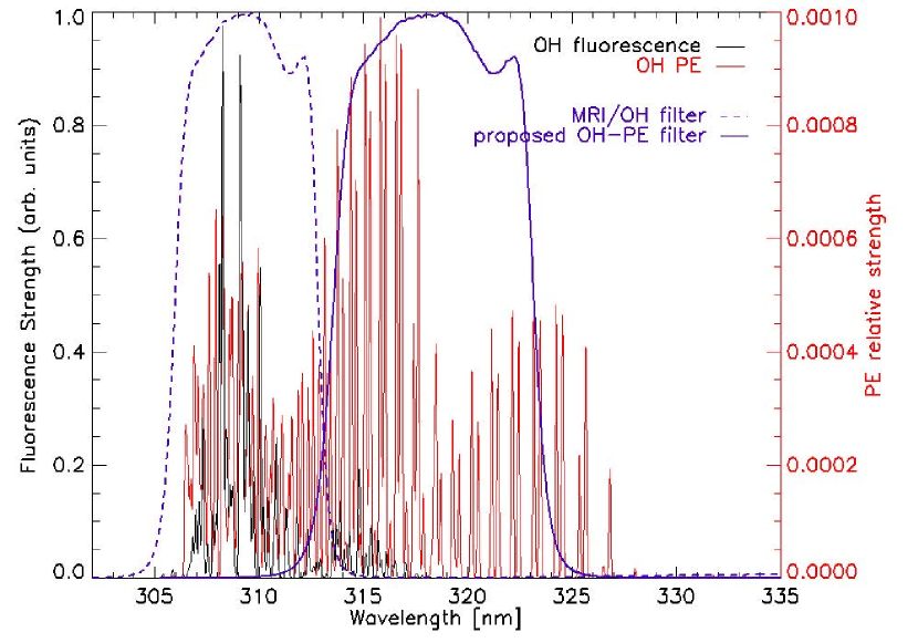
Figure 20: Bandpass of the proposed OH-PE dedicated filter (solid line) shifted and scaled with respect to MRI-OH filter (dashed line) to have $\lambda_{c}=$318.8 nm and $\Delta\lambda=$8.7 nm to maximize prompt emission (red spectrum) contribute and minimize flurescence emission (black spectrum) contribute.

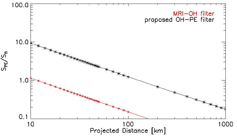
Figure 21: Relative strenght of OH-PE to RFE emission as function of the projected distance from the nucleus as seen through MRI-OH filter (red) and the proposed OH-PE dedicated filter.

We demonstrated that a dedicated OH-PE filter could be used to directly image the distribution of H₂O in the inner coma when the first 200 km of the inner coma can be resolved. OH* prompt emission traces water better than forbidden [OI] emission which is more difficult to interpret (see for example Bodewits et al. 2016) because it can have multiple parents (H₂O, CO₂, CO, and O₂), and because the long lifetime of the ¹D state leads to transport and quenching.

We tentatively performed an optimization of the design of such a filter using MRI-OH filter profile shifted and scaled to minimize the contribution of fluorescence while maximizing prompt emission. In Table 1 we listed the percentage of total fluorescence (RFE) and the percentage of total prompt emission (PE) passing through the filter for each combination of central wavelength ($\lambda_{c}$) and bandwidth ($\Delta\lambda$). The first line shows the values for MRI-OH filter. The two bands are partially superimposed, therefore a complete exclusion of fluorescence is difficult unless a sharper filter cutoff is used at low wavelenghts. The best solution for a filter profile similar to MRI-OH is given by a filter centered at 318.8 nm with bandwidth of 8.7 nm (Fig. 20) which would include 12.1% of total fluorescence emission and 46.3% of total prompt emission. This is considered the best compromise to include the PE peak and exclude as much fluorescence as possible.

We computed the relative strenght of the two bands for the conditions at Hartley 2 through such a filer (Fig. 21). For comparison the relative strenght through MRI-OH filter is also shown. Fig. 21 revelas that through such OH-PE dedicated filter the prompt emission would be ten times stronger than fluorescence in the inner coma, at about 10 km from the nucleus. This result confirms the importance of including a dedicated OH-PE filter in the payload of future missions to comets to allow a direct measurement of the distribution of water at optical waveleghts.

References

- A’Hearn et al. (2015) A’Hearn, M. F., Krishna Swamy, K. S., Wellnitz, D. D., & Meier, R. 2015, AJ, 150, 5
- A’Hearn et al. (1995) A’Hearn, M. F., Millis, R. C., Schleicher, D. O., Osip, D. J., & Birch, P. V. 1995, Icarus, 118, 223
- A’Hearn et al. (1983) A’Hearn, M. F., Schleicher, D. G., & Feldman, P. D. 1983, ApJ, 274, L99
- A’Hearn et al. (2011) A’Hearn, M. F., Belton, M. J. S., Delamere, W. A., et al. 2011, Science, 332, 1396
- Becker & Haaks (1973) Becker, K. H., & Haaks, D. 1973, Z. Naturforsch. A, 28, 149
- Belton et al. (2013) Belton, M. J. S., Thomas, P., Li, J.-Y., et al. 2013, Icarus, 222, 595
- Bertaux (1986) Bertaux, J. L. 1986, A&A, 160, L7
- Bhardwaj et al. (1996) Bhardwaj, A., Haider, S. A., & Singhal, R. P. 1996, Icarus, 120, 412
- Biver et al. (1999) Biver, N., Bockelée-Morvan, D., Crovisier, J., et al. 1999, AJ, 118, 1850
- Bockelee-Morvan & Crovisier (1985) Bockelee-Morvan, D., & Crovisier, J. 1985, A&A, 151, 90
- Bockelée-Morvan et al. (2004) Bockelée-Morvan, D., Crovisier, J., Mumma, M. J., & Weaver, H. A. 2004, The composition of cometary volatiles, ed. G. W. Kronk, 391–423
- Bodewits et al. (2016) Bodewits, D., Lara, L. M., A’Hearn, M. F., et al. 2016, AJ, 152, 130
- Bonev et al. (2004) Bonev, B. P., Mumma, M. J., Dello Russo, N., et al. 2004, ApJ, 615, 1048
- Bonev et al. (2006) Bonev, B. P., Mumma, M. J., DiSanti, M. A., et al. 2006, ApJ, 653, 774
- Brooke et al. (1996) Brooke, T. Y., Tokunaga, A. T., Weaver, H. A., et al. 1996, Nature, 383, 606
- Budzien & Feldman (1991) Budzien, S. A., & Feldman, P. D. 1991, Icarus, 90, 308
- Carrington (1964) Carrington, T. 1964, The Journal of Chemical Physics, 41
- Chamberlain & Hunten (1987) Chamberlain, J. W., & Hunten, D. M. 1987, Theory of planetary atmospheres. An introduction to their physics and chemistry.
- Combi et al. (2004) Combi, M. R., Harris, W. M., & Smyth, W. H. 2004, Gas dynamics and kinetics in the cometary coma: theory and observations, ed. G. W. Kronk, 523–552
- Combi & Smyth (1988) Combi, M. R., & Smyth, W. H. 1988, ApJ, 327, 1026
- Crifo et al. (2004) Crifo, J. F., Fulle, M., Kömle, N. I., & Szego, K. 2004, Nucleus-coma structural relationships: lessons from physical models, ed. M. C. Festou, H. U. Keller, & H. A. Weaver, 471–503
- de Almeida & Singh (1986) de Almeida, A. A., & Singh, P. D. 1986, Earth Moon and Planets, 36, 117
- Edberg et al. (2015) Edberg, N. J. T., Eriksson, A. I., Odelstad, E., et al. 2015, Geophys. Res. Lett., 42, 4263
- Farnham (2009) Farnham, T. L. 2009, Planet. Space Sci., 57, 1192
- Farnham et al. (2000) Farnham, T. L., Schleicher, D. G., & A’Hearn, M. F. 2000, Icarus, 147, 180
- Feldman et al. (2015) Feldman, P. D., A’Hearn, M. F., Bertaux, J.-L., et al. 2015, A&A, 583, A8
- Festou (1981) Festou, M. C. 1981, A&A, 96, 52
- Fray et al. (2005) Fray, N., Bénilan, Y., Cottin, H., Gazeau, M.-C., & Crovisier, J. 2005, Planet. Space Sci., 53, 1243
- Gibb et al. (2003) Gibb, E. L., Mumma, M. J., Dello Russo, N., DiSanti, M. A., & Magee-Sauer, K. 2003, Icarus, 165, 391
- Hampton et al. (2005) Hampton, D. L., Baer, J. W., Huisjen, M. A., et al. 2005, Space Sci. Rev., 117, 43
- Harich et al. (2000) Harich, S. A., Hwang, D. W. H., Yang, X., et al. 2000, The Journal of Chemical Physics, 113
- Haser (1957) Haser, L. 1957, Bull. Acad. R. de Belgique, Classe de Sci., 43
- Jewitt & Meech (1986) Jewitt, D., & Meech, K. J. 1986, ApJ, 310, 937
- Keller et al. (2007) Keller, H. U., Barbieri, C., Lamy, P., et al. 2007, Space Sci. Rev., 128, 433
- Kelley et al. (2013) Kelley, M. S., Lindler, D. J., Bodewits, D., et al. 2013, Icarus, 222, 634
- Kim et al. (1990) Kim, S. J., A’Hearn, M. F., & Larson, S. M. 1990, Icarus, 87, 440
- Klaasen et al. (2008) Klaasen, K., A’Hearn, M. F., Baca, M., et al. 2008, Review of Scientific Instruments, 79, 77
- Klaasen et al. (2013) Klaasen, K. P., A’Hearn, M., Besse, S., et al. 2013, Icarus, 225, 643
- Knight et al. (2015) Knight, M. M., Mueller, B. E. A., Samarasinha, N. H., & Schleicher, D. G. 2015, AJ, 150, 22
- Knight & Schleicher (2013) Knight, M. M., & Schleicher, D. G. 2013, Icarus, 222, 691
- Laffont et al. (1998) Laffont, C., Boice, D. C., Moreels, G., et al. 1998, Geophys. Res. Lett., 25, 2749
- Lara et al. (2011) Lara, L. M., Lin, Z.-Y., & Meech, K. 2011, A&A, 532, A87
- Li et al. (2013) Li, J.-Y., Besse, S., A’Hearn, M. F., et al. 2013, Icarus, 222, 559
- Luque & Crosley (1999) Luque, J., & Crosley, D. R. 1999, SRI International Report, MP 99
- McLaughlin et al. (2011) McLaughlin, S. A., Carcich, B., Sackett, S. E., & Klaasen, K. P. 2011, EPOXI 103P/Hartley 2 Encounter - MRI Calibrated Images v1.0,DIF-C-MRI-3/4-EPOXI-HARTLEY2-v1.0, NASA Planetary Data System
- Mordaunt et al. (1994) Mordaunt, D. H., Ashfold, M. N. R., & Dixon, R. N. 1994, J. Chem. Phys., 100, 7360
- Mumma et al. (2001) Mumma, M. J., McLean, I. S., DiSanti, M. A., et al. 2001, ApJ, 546, 1183
- Protopapa et al. (2014) Protopapa, S., Sunshine, J. M., Feaga, L. M., et al. 2014, Icarus, 238, 191
- Samarasinha & Larson (2011) Samarasinha, N. H., & Larson, S. M. 2011, in EPSC-DPS Joint Meeting 2011, 1400
- Schleicher & A’Hearn (1982) Schleicher, D. G., & A’Hearn, M. F. 1982, ApJ, 258, 864
- Schleicher & A’Hearn (1988) —. 1988, ApJ, 331, 1058
- Schleicher & Farnham (2004) Schleicher, D. G., & Farnham, T. L. 2004, Photometry and imaging of the coma with narrowband filters, ed. M. C. Festou, H. U. Keller, & H. A. Weaver, 449–469
- Swings (1941) Swings, P. 1941, Lick Observatory Bulletin, 19, 131
- Tenishev et al. (2008) Tenishev, V., Combi, M., & Davidsson, B. 2008, ApJ, 685, 659
- Thomas et al. (2013) Thomas, P. C., A’Hearn, M. F., Veverka, J., et al. 2013, Icarus, 222, 550
- Turner & Smith (1999) Turner, N. J., & Smith, G. H. 1999, AJ, 118, 3039
- Weaver et al. (1996) Weaver, H. A., Feldman, P. D., A’Hearn, M. F., et al. 1996, in Bulletin of the American Astronomical Society, Vol. 28, American Astronomical Society Meeting Abstracts #188, 925
- Williams et al. (2012) Williams, J. L., Li, J.-Y., Bodewits, D., & McLaughlin, S. A. 2012, NASA Planetary Data System
- Woodney et al. (2002) Woodney, L. M., A’Hearn, M. F., Schleicher, D. G., et al. 2002, Icarus, 157, 193
- Yamashita (1975) Yamashita, I. 1975, J. Phys. Soc. Jpn., 39, 205