Probing photospheric magnetic fields with new spectral line pairs

Abstract

Context. The magnetic line ratio (MLR) method has been extensively used in the measurement of photospheric magnetic field strength. It was devised for the neutral iron line pair at 5247.1 Å and 5250.2 Å (5250 Å pair). Other line pairs as well-suited as this pair been have not been reported in the literature.

Aims. The aim of the present work is to identify new line pairs useful for the MLR technique and to test their reliability.

Methods. We use a three dimensional magnetohydrodynamic (MHD) simulation representing the quiet Sun atmosphere to synthesize the Stokes profiles. Then, we apply the MLR technique to the Stokes $V$ profiles to recover the fields in the MHD cube both, at original resolution and after degrading with a point spread function. In both these cases, we aim to empirically represent the field strengths returned by the MLR method in terms of the field strengths in the MHD cube.

Results. We have identified two new line pairs that are very well adapted to be used for MLR measurements. The first pair is in the visible, Fe i 6820 Å–6842 Å (whose intensity profiles have earlier been used to measure stellar magnetic fields), and the other is in the infrared (IR), Fe i 15534 Å–15542 Å. The lines in these pairs reproduce the magnetic fields in the MHD cube rather well, partially better than the original 5250 Å pair.

Conclusions. The newly identified line pairs complement the old pairs. The lines in the new IR pair, due to their higher Zeeman sensitivity, are ideal for the measurement of weak fields. The new visible pair works best above $300$ G. The new IR pair, due to its large Stokes $V$ signal samples more fields in the MHD cube than the old IR pair at $1.56\,\mu$m, even in the presence of noise, and hence likely also on the real Sun. Owing to their low formation heights (100–200 km above $\tau_{5000}=1$), both the new line pairs are well suited for probing magnetic fields in the lower photosphere.

1 Introduction

Spectral lines offer diagnostics to measure magnetic fields on the Sun. Accurate magnetic field measurement relies on an optimal combination of spectral lines and the method employed to extract the information on the field. Unfortunately, the Stokes profiles $(I,Q,U,V)$ are affected by many other atmospheric parameters besides the field, making the extraction of the field complex and time consuming. To bypass this, at least for the field strength, Stenflo (1973) proposed the magnetic line ratio (MLR) method which involves determining the intrinsic magnetic field strength ($B$) from the ratio of Stokes $V$ of two lines. The two spectral lines must form under the same atmospheric conditions but differ in their magnetic sensitivities, given by the effective Landé g-factors (g_eff). For weak, height-independent fields, the Stokes $V$ ratio is simply equal to the ratio of their g_eff. In the presence of strong height-independent fields, the ratio saturates and becomes independent of $B$. This method works best for intermediate field strengths where the Stokes $V$ ratio is proportional to $B$, due to the differential Zeeman saturation. Stenflo (1973) applied MLR to the line pair Fe i 5247.1 Å–5250.2 Å (5250 Å pair) in the photospheric network which lead to the discovery of the presence of kilo-Gauss (kG) fields. Since then the MLR has been widely used to measure photospheric magnetic fields (Stenflo & Harvey 1985; Solanki et al. 1987; Schüssler & Solanki 1988; Solanki et al. 1992; Keller et al. 1994; Grossmann-Doerth et al. 1998; Lozitsky et al. 1999; Stenflo 2010, 2011). For reviews on MLR see Solanki (1993, 2009); de Wijn et al. (2009); Stenflo (2013).

In addition to the MLR, line pairs formed at similar heights in the atmosphere but with different g_eff are used in multi-line inversions to measure magnetic field. Two other spectral line pairs, used for inversions as well as MLR, are the 6301.5 Å–6302.5 Å (6300 Å pair) in the visible (Domínguez Cerdeña et al. 2003a, b; Stenflo 2010; Ishikawa & Tsuneta 2011; Steiner & Rezaei 2012), and the 15648.5 Å–15652.8 Å ($1.56\,\mu$m pair) in the infrared (IR, e.g., Solanki et al. 1996). The $1.56\,\mu$m pair was identified by Solanki et al. (1992) and has been used in the measurement of internetwork fields (Lin 1995; Solanki et al. 1996; Khomenko et al. 2003; Martínez González et al. 2007; Lagg et al. 2016). The 6300 Å pair is used to study both quiet and active regions on the Sun (for e.g., Domínguez Cerdeña et al. 2003a, b; Socas-Navarro & Sánchez Almeida 2002, 2003; Socas-Navarro et al. 2004; Martínez González et al. 2006; Centeno et al. 2007; Lites et al. 2008), based on the observations from both ground based telescopes and the Hinode satellite. The distribution of the quiet Sun photospheric magnetic field revealed by these two line pairs is quite different, particularly in the internetwork, first observed by Sánchez Almeida et al. (2003). The $1.56\,\mu$m pair indicates the presence of mostly sub-kG fields while the 6300 Å pair indicates kG fields. Combined analyses of the two line pairs have been carried out by Socas-Navarro & Sánchez Almeida (2003); Khomenko et al. (2005); Domínguez Cerdeña et al. (2006), although with contradictory results.

Table 1: Atomic parameters of the new and the old line pairs.

New pairs
	Wavelength (Å)	Element	$J_{l}$	$J_{u}$	log($gf$)	$\chi_{e}$ (e.v.)	gl	gu	geff
I	6820.3715	Fe i	1.0	2.0	-1.32	4.63	2.5	1.83	1.5
	6842.6854	Fe i	1.0	1.0	-1.32	4.63	2.5	2.5	2.5
II	6213.4291	Fe i	1.0	1.0	-2.48	2.22	2.5	1.5	2.0
	6219.2802	Fe i	2.0	2.0	-2.43	2.19	1.83	1.5	1.67
III	15534.257	Fe i	1.0	2.0	-0.382	5.64	1.5	1.83	2.0
	15542.089	Fe i	1.0	0.0	-0.337	5.64	1.5	0.0	1.50
Old pairs
	Wavelength (Å)	Element	$J_{l}$	$J_{u}$	log($gf$)	$\chi_{e}$ (e.v.)	gl	gu	geff
I	5247.0504	Fe i	2.0	3.0	-4.946	0.087	1.5	1.75	2.0
	5250.2080	Fe i	0.0	1.0	-4.938	0.121	0.0	3.0	3.0
II	6301.5012	Fe i	2.0	2.0	-0.718	3.654	1.83	1.5	1.67
	6302.4936	Fe i	1.0	0.0	-1.236	3.686	2.5	0.0	2.5
III	15648.518	Fe i	1.0	1.0	-0.675	5.426	3.0	3.0	3.0
	15652.874	Fe i	5.0	4.0	-0.043	6.246	1.51	1.49	1.53
IV	4122.8020	Fe i	2.0	3.0	-1.300	2.832	1.50	1.16	0.820
	8999.5600	Fe i	2.0	2.0	-1.300	2.832	1.50	1.49	1.496

Khomenko & Collados (2007) applied MLR to the above three line pairs synthesized from a three dimensional magnetohydrodynamic (3D MHD) snapshot. They concluded in favour of the $1.56\,\mu$m and the 5250 Å pairs, although they could not recover kG from the 5250 Å pair. The 6300 Å pair does not reproduce the fields in the MHD cube, due to the difference in height of formation (HOF) of the two lines (Shchukina & Trujillo Bueno 2001; Khomenko & Collados 2007; Grec et al. 2010). Discrepancies in the results from the 6300 Å pair observations have been reported in Domínguez Cerdeña et al. (2003b); Martínez González et al. (2006). In a contrasting study, Socas-Navarro et al. (2008), concluded that the 6300 Å pair is better than the 5250 Å pair, as they could not recover kG fields in the network observations from the 5250 Å pair. In Section 5 of the present paper, we try to provide an explanation for this discrepancy. In order to compensate for the difference in HOF of the 6300 Å pair, Stenflo (2010); Stenflo et al. (2013) devised a renormalization to the MLR of 6300 Å pair in terms of the 5250 Å pair.

Any differences in the HOF of the lines in a pair increase the difficulties in interpreting the results from the MLR. The formation heights of the lines in 6300 Å pair are separated by more than 100 km and those in the $1.56\,\mu$m pair by $\approx 30$km. These issues leave us with a single “ideal” line pair (Stenflo et al. 2013) for the MLR. Socas-Navarro et al. (2007, 2008) proposed that the pair 4122 Å–9000 Å works better than all the above pairs (i.e., pairs I, II and III in the lower part of Table 1). However these lines are 5000 Å apart and need to be observed simultaneously. Also, the Landé g-factor of the 4122 Å is quite low (see Table 1) and hence this line is less sensitive to magnetic fields. A survey of the Fe i lines with different magnetic sensitivities was carried out by Vasilyeva & Shchukina (2009). They present a list of 28 line pairs which are suitable for MLR. However most of them are quite weak and the authors do not discuss the reliability of these pairs in detail.

After a detailed search in the visible and IR range of the solar spectrum, we have identified three new line pairs. Two pairs are in the visible at 6820 Å–6842 Å (6842 Å pair) and 6213 Å-6219 Å (6219 Å pair). The third pair is in the IR at 15534 Å–15542 Å ($1.55\,\mu$m pair). The lines in each pair have identical/similar atomic parameters but different g_eff. We find that the 6842 Å and the $1.55\,\mu$m pairs are more suitable for MLR than the 6219 Å pair. The lines in these two pairs are formed deep in the photosphere. We compare the performance of the new and the old line pairs by applying the MLR method to the Stokes profiles in a 3D MHD cube, and by comparing the results with the fields in the cube. This is done at both original resolution of the cube and after applying a degradation. In the first case, we show that the magnetic field strengths given by MLR are best represented when the field strengths in the MHD cube are weighted by the response functions of Stokes $V$ profiles and then integrated over the optical depth. In the presence of instrumental degradation, this is quite challenging. In this paper, we have made the first attempt to empirically represent the magnetic field strengths returned by the MLR method in a realistic atmosphere with realistic degradation.

In Section 2, we discuss the atomic parameters of the new lines. In Section 3, we compute their HOF from the response functions. A detailed comparison between the $B$ from the MLR and the MHD cube is presented in Section 4. In Section 5, we repeat the analyses by spatially and spectrally degrading the Stokes profiles and present the conclusions in Section 6.

2 Atomic parameters

The new and the old line pairs are listed in Table 1. The atomic parameters are taken from Kurucz, NIST and VALD atomic databases.

The newly identified pairs have been listed in Solanki & Stenflo (1985); Solanki et al. (1992); Ramsauer et al. (1995). The intensity profiles of the 6842 Å line pair has earlier been used by Rüedi et al. (1997) to measure the magnetic fields on cool dwarfs using inversions. Due to its large g_eff, the 6842 Å line is used by Balthasar & Schmidt (1993); Wiehr (2000) to study sunspots and filaments. Furthermore, the 6842 Å line in combination with Fe i 6843 Å line was used by Saar et al. (1994) to measure magnetic fields in late-type stars. The two lines in the 6842 Å are separated by 22 Å and are unblended. They have identical oscillator strengths (log$(gf)$) and excitation potentials ($\chi_{e}$) with very different g_eff. In the absence of a magnetic field, the lines are formed at the same height in the atmosphere and further details will be discussed in Section 3.2. Due to their high excitation potential, these lines are less sensitive to fluctuations in $T$ than the 5250 Å pair.

The lines in the 6219 Å pair, have the same log($gf$) and nearly same $\chi_{e}$. Though they are formed at the same height in the atmosphere for $B=0$, their g_eff differ by only 20%, rendering them non-ideal for MLR. The third new pair is in the IR, separated by 8 Å at 15534 Å–15542 Å. They belong to different multiplets but have the same $\chi_{e}$ and similar log($gf$). The red wing of the 15534 Å line is affected by a minor unidentified blend which, may not significantly affect the Stokes $V$ profiles. The blue wing is clean without any blends. The 15542 Å line has no visible blends in the solar spectrum, however, Solanki et al. (1990) indicate the presence of three Mg i blends. These three Mg i lines have not been listed in the Kurucz, NIST or VALD atomic databases and appear to have been present only in older databases, so that they may be spurious. According to Ramsauer et al. (1995) this line is only lightly blended by a Si i line at 15542.016 Å.

The new line pairs in the visible and IR are separated by 22 Å and 8 Å, respectively. The IR pair can be observed with the GREGOR Infrared Spectrograph (GRIS; Collados et al. 2012) as spectral range as wide as 20 Å has been observed with this instrument (Lagg et al. 2016). It is possible to cover the 22 Å range of the visible line pair using 2k x 2k detector at a spectral resolving power of 270000 or better. The new line pairs can be observed with the spectro-polarimeters at the upcoming Daniel K. Inouye Solar Telescope (DKIST) such as the Visible Spectro-Polarimeter (ViSP; Elmore et al. 2014) and the Diffraction Limited Near Infrared Spectro-Polarimter (DL-NIRSP; Elmore et al. 2014).

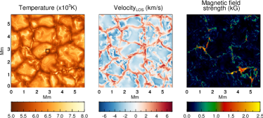
Figure 1: The temperature, line-of-sight (LOS) velocity and magnetic field maps of the MURaM MHD cube at log($\tau_{5000})=0$. The cube has an average unsigned LOS magnetic field of 50 G. The black box near the center of the first panel represents the area over which the Stokes profiles in Figure 2 are averaged. The size of the box is $0.4^{\prime\prime}\times 0.4^{\prime\prime}$.

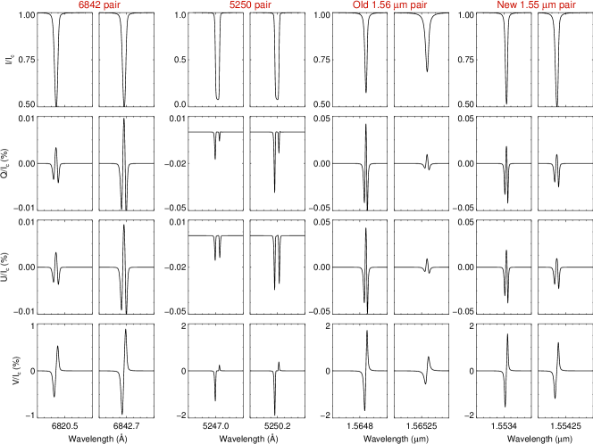
Figure 2: Stokes profiles of the four line pairs from the MHD cube, averaged over a box of size $0.4^{\prime\prime}\times 0.4^{\prime\prime}$. The location of the box is shown in the first panel of Figure 1.

3 Height of formation

3.1 3D MHD cube and profile synthesis

We use a snapshot of a 3D MHD simulation computed from the MURaM code (Vögler et al. 2005). We have selected a cube from the set used by Riethmüller et al. (2014) but with a different resolution. The size of the cube is (6 $\times$ 6 $\times$ 1.4) Mm with a resolution of (20.83 $\times$ 20.83 $\times$ 14) km. The cube has an unsigned average line-of-sight (LOS) magnetic field of 50 G. The properties of the cube, such as the temperature ($T$), LOS velocity ($\varv_{\rm LOS}$), and $B$ at log($\tau_{5000}$)=0 are shown in Figure 1. The cube represents the quiet Sun atmosphere, dominated by weak and intermediate fields. However there are a few patches of strong magnetic fields in the lower right corner and in the mid-left, as seen from Figure 1. The Stokes profiles are synthesized using the Stokes-Profiles-INversion-O-Routines (SPINOR) of Frutiger et al. (2000); Frutiger (2000), run in its forward mode along each vertical column of the MHD cube (1.5D) at a heliocentric angle of $\mu=1$.

In Figure 2, we present the Stokes profiles of all the four line pairs spatially averaged over a small region of $0.4^{\prime\prime}\times 0.4^{\prime\prime}$ close to the center of the analyzed MHD snapshot, indicated by the black box in the first panel of Figure 1. The size of the averaged area is chosen to match the resolution of recent observations at the GREGOR telescope (Schmidt et al. 2012) with the GREGOR Infrared Spectrograph (GRIS) instrument (Collados et al. 2012) such as those presented in Lagg et al. (2016).

In the visible range, the new 6842 Å pair is weaker than the 5250 Å pair in both intensity and polarization (note the different vertical scales). However, in the IR, though the 15648 Å line of the old IR pair is strong and has large Stokes amplitudes ($Q,U,V$), the 15652 Å line has much weaker amplitudes, especially in $Q$ and $U$ (see also Martínez González et al. 2008; Lagg et al. 2016) than the lines of the new pair. This makes it harder to use the lines of the old IR pair together, in MLR as well as in inversions when the profiles are affected by noise. In this respect, the new $1.55\,\mu$m pair offers great advantage as both the lines have large Stokes amplitudes. The strong linear polarization signals can be particularly favourable for measuring vector magnetic fields using inversions.

3.2 Response functions

To compare the HOF of the line pairs, we use Response Functions (RFs, Beckers & Milkey 1975). These functions measure the responses of the line profiles to variations in atmospheric properties such as $T$, $\varv_{\rm LOS}$ and $B$. Using the SPINOR code, we compute the RFs of the Stokes $I$ and $V$ profiles of all the lines to these three atmospheric properties. For the Stokes $I$ profiles, we use the RF at the line center wavelength and for Stokes $V$, we use the RF at the wavelength corresponding to the largest peak in the $V$ profile. This is because later, in section 4, we compute the MLR from this largest peak, also referred to as the prominent peak. The HOF is then assumed to be at the centroid of the RFs. The distribution of the HOF across the cube, for different spectral lines, from RFs of Stokes $I$ and $V$ profiles to $T$ are shown in the first two rows of Figures 3 and 5, respectively. The third row is the unsigned difference in the HOF ($\delta$HOF) between the lines in the pair. The histograms of the distribution of HOF and $\delta$HOF are shown in the last two rows. The reference height $z=0$ km corresponds to the geometrical layer where log$(\tau_{5000})$, on average, is zero. This HOF represents the atmospheric height that is most sampled by the spectral line. In other words, the Stokes profiles are strongly influenced by the physical conditions at the HOF of the line.

Though $T$ has a dominant influence on the spectral lines and their formation, the RFs from $\varv_{\rm LOS}$, $B$ and magnetic field inclination ($\gamma$) also provide valuable information, especially for the MLR. Gradients in the $\varv_{\rm LOS}$, $B$ and $\gamma$ affect the shapes of the Stokes $V$ profiles, resulting in asymmetries (Khomenko et al. 2005). Hence, the MLR works best if the two lines sample the same $\varv_{\rm LOS}$, $B$ and $\gamma$, in addition to $T$. To confirm this, we have computed the $\delta$HOF for each line pair from the RFs of Stokes $I$ and $V$ profiles to $\varv_{\rm LOS}$, $B$, and $\gamma$ RFs, in the same way as we did for the $T$ RFs. The variations in $\delta$HOF and the histograms are shown in Figures 4 and 6.

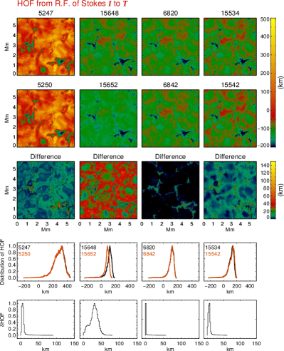
Figure 3: Maps of height of formation (HOF) for different line pairs deduced from the centroid of the response function (RF) of Stokes $I$ profiles to temperature, at the central wavelength. First and second rows: distribution of HOF referring to individual spatial pixels of the MHD cubes. Third row: difference (absolute) in the HOF. Forth row: histogram of the HOF of the two lines in each pair. Fifth row: histogram of the absolute differences in the HOF.

3.2.1 Old pairs

From the $T$ RFs of Stokes $I$ (Figure 3), the 5247 Å and 5250 Å lines are formed at similar heights in the atmosphere for $B=0$ and for weak fields. The histograms of the distribution of HOFs obtained for vertical rays passing through each horizontal pixel of the MHD snapshot for both the lines almost entirely overlap and peak around 300 km and the $\delta$HOF has a narrow spread with a peak at 20 km. They start to differ for intermediate and strong fields where the $\delta$HOF can be as high as 100 km. These pixels correspond mostly to the edges of granules to intergranular lanes. In regions of strong magnetic field concentrations (seen at bottom right and mid-left of the atmosphere), not only the HOF of both lines decrease due to plasma evacuation leading to a drop in the gas pressure, the $\delta$HOF also increases due to the difference in Landé factor. The histograms of the $\delta$HOF deduced from $\varv_{\rm LOS}$, $B$ and $\gamma$ RFs of Stokes $I$ profiles at the line center (Figure 4), peak close to zero and at a few pixels reach values as high as 150 km in the strong magnetic regions. Differences in HOF are also seen in the regions surrounding the strong field concentrations because of the magnetic canopies, leading to the measurement of stronger $B$ from MLR (Section 4, see also Khomenko & Collados 2007).

The $T$ RFs of Stokes $I$ profiles (Figure 3) of the 1.56 $\mu$m pair indicate that the two lines are most commonly formed around 30 km apart. However this difference decreases for the $\varv_{\rm LOS}$, $B$ and $\gamma$ RFs (Figure 4). In particular, the two lines sample similar $B$, despite the difference in their HOFs from the $T$ RFs of Stokes $I$ profiles.

From the Stokes $V$ profiles, since the RFs are considered at the wavelengths of the prominent peak which is away from the line center, the HOFs are slightly lower in the atmosphere, especially for the 5250 Å pair (Figure 5). For the $1.56\,\mu$m pair, the distribution of the HOFs from Stokes $V$ profiles in Figure 5 nearly overlap, unlike from the Stokes $I$ profiles (Figure 3). Other than these difference, the overall distribution of the HOFs and the $\delta$HOF from $T,\varv_{\rm LOS},B$ and $\gamma$ RFs are similar to the case of RFs for Stokes $I$, although in general the difference in the HOFs is now smaller, implying that the MLR should work better than suggested by Figures 3 and 4 alone.

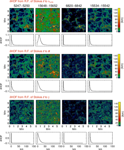
Figure 4: Maps of difference in heights of formation and their histograms. They are similar to the third and fifth rows of Figure 3, but computed from the RFs of Stokes $I$ profiles to perturbations in velocity, magnetic field strength, and inclination.

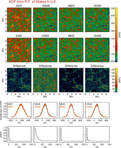
Figure 5: Maps of height of formation for different spectral lines deduced from the centroid of the response function of Stokes $V$ profiles to temperature at the wavelength corresponding to the largest peak in $V$. Different rows represent the same quantities as in Figure 3.

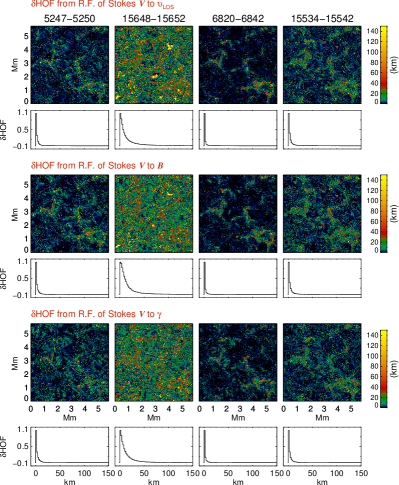
Figure 6: Maps of difference in heights of formation and their histograms, similar to Figure 4, but computed from the response functions of Stokes $V$ profiles to perturbations in velocity, magnetic field strength, and inclination.

3.2.2 New pairs

Lines in the newly identified 6842 Å pair sample the same heights over most of the atmosphere , evident from the maps of HOFs deduced from the RFs of both Stokes $I$ and $V$ profiles to different atmospheric properties. Like the other pairs, this changes in the strong magnetic regions, with differences in HOF $>50$ km at some pixels, unavoidably caused by the different Landé factors of the two lines. However, unlike the other line pairs, the $\delta$HOF for the new pair always peaks at zero, with a narrow spread in all the different cases shown in Figures 3 – 6. This makes the line pair most suitable for the MLR method, of all the considered pairs, at least in this respect. Also, the pair is formed around 100 km above log$(\tau_{\rm 5000})=0$ and samples deep photospheric layers similar to the old 1.56 $\mu$m pair. Thus we now have a line pair in the visible, which can be used complementarily with the IR pair to probe the deep photospheric layers. In addition, the spread in the HOF of the 6842 Å pair is small and their individual RFs are quite narrow implying that they see a narrow range of atmospheric layers due to their higher excitation potentials, unlike the 5250 Å pair. This makes them less sensitive to magnetic field gradients, which is an advantage for the line ratio, but a disadvantage for their use in height-dependent inversions. Similar is the case with the new 1.55 $\mu$m pair. The two lines are formed at the same height, deep in the photosphere, as seen in the maps of HOFs from the RFs of both Stokes $I$ and $V$ profiles (Figures 3 – 6). Particularly in the granules, their $\delta$HOF is close to zero. Due to the increased Zeeman sensitivity of the IR lines, this pair is well suited for the measurement of weak granular fields, as will be discussed in Section 4. Also, notice the similarity in HOF of the new IR pair and the 15648 Å (g_eff=3) line from the old IR pair. If two wavelength ranges can be covered simultaneously, then the two IR pairs, with their very different magnetic sensitivities, can be used together.

4 Comparison with the 3D MHD simulations

We define the MLR of a line pair as the ratio of Stokes $V$ amplitude from the magnetically weaker line (smaller g_eff) to the stronger line (higher g_eff), similar to Khomenko & Collados (2007). To extract $B$ from this ratio, we need a calibration curve. Though neither micro- nor macro-turbulent velocities ($\varv_{\rm mic,mac}$) are used in the computation of the Stokes profiles, they are still broadened by the often strong vertical gradients in $\varv_{\rm LOS}$. Hence we must account for the widths of the spectral lines in the construction of the calibration curves. In Figure 7, we show the distribution of the line widths, defined in this case as the full width at half maximum (FWHM), for lines in the four pairs. Except for the old $1.56\,\mu$m pair, the lines in each pair have practically the same line widths. The difference in line widths is a product of the difference in HOF between the lines in the $1.56\,\mu$m pair.

Ideally, before applying the MLR, one must construct calibration curves at every pixel by fitting the intensity profiles using both micro and macro-turbulence, for the four line pairs. This increases the number of calibration curves and they are not unique, as different combinations of micro- and macro-turbulence are possible. In order to simplify this, we first set $\varv_{\rm mac}=0$ and match the line widths using $\varv_{\rm mic}$. We then divide the range of line widths into ten bins, of size 3 mÅ for the visible pairs and 10 mÅ for the IR pairs. We vary a height-independent $\varv_{\rm mic}$ from 0.0 to 3.5 km/s to get the required line width and construct a calibration curve for each width bin and each line pair. Figure 8 shows the resulting calibration curves for each line pair. The curves are computed using the HSRA (Gingerich et al. 1971) model atmosphere. Fitting both line width and depth by varying $\varv_{\rm mac}$ and $\varv_{\rm mic}$ will increase the number of calibration curves. Setting $\varv_{\rm mac}=0$ is a choice made to minimize the number of calibration curves. Despite this simplification, we recover the magnetic field strengths in the MHD cube relatively well, as discussed below.

The calibration curves for the 6842 Å pair, in Figure 8, starts to decrease below the saturation level once the field strength exceeds a certain threshold value ($B_{\rm th}$). The greater the turbulent velocity or the wider the spectral line, the higher is the value of $B_{\rm th}$. In the absence of any turbulent velocity (first calibration curve for the 6842 Å pair), $B_{\rm th}\approx 1200$ G. Similarly, the calibration curves for the new $1.55\,\mu$m pair continues to increase beyond unity when the field strength exceeds $B_{\rm th}$ for that pair. This is because of the anomalous Zeeman splitting of the spectral lines. We discuss this in greater detail in the appendix.

The ambiguities involved in the comparison of $B$ from MLR with the 3D MHD cube are more severe than those involved while comparing the inversion results with the MHD simulations. The later case has been discussed in detail in Borrero et al. (2014). For the MLR, a similar comparison is made by Khomenko & Collados (2007). In this paper, the authors compare the results from MLR with $B$ at log($\tau_{5000})$=-1 layer in the MHD cube. For only a slice of the cube, they also discuss the comparison with the fields weighted by the response function of Stokes $I$ to $T$. As the lines sample different depths across the cube (Figures 3 – 6), comparing the results of MLR with the fields at constant $\tau$ will not properly indicate the reliability of the line pair. Hence, we discuss below a different way of comparing $B$ from MLR and the MHD cube.

Traditionally, the MLR is computed by either taking the ratio of the blue Stokes $V$ peak, as done in, e.g. Khomenko & Collados (2007); Stenflo (2010); Stenflo et al. (2013), or by taking the sum or the average of the blue and the red lobes (e.g., Stenflo & Harvey 1985; Solanki et al. 1987). The rationale behind the former is that the blue peak is less affected by magnetic and velocity gradients, and that they have larger amplitudes (Stenflo 2010). Taking the sum or the average of the blue and the red lobes improves the signal to noise ratio. However, while comparing with the magnetic field strength in the MHD cube, we find that the ratio of the most prominent peak (the lobe with higher amplitude) in the Stokes $V$ profile performs better than the other two ratios. A similar approach has also been followed by Lagg et al. (2016).

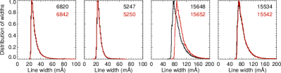
Figure 7: Distribution of line widths in the four line pairs across the cube.

Figure 8: Ten calibration curves for each line pair, one for each of the ten bins into which the line widths are divided. The curves are computed for the HSRA model by varying height-independent micro-turbulent velocity from 0.0 km/s to 3.5 km/s.

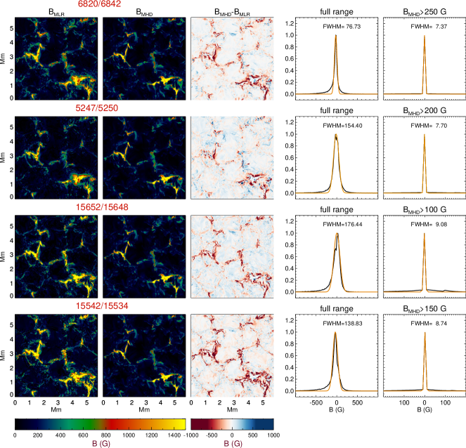
Figure 9: Comparison between the magnetic field strengths from the MLR ($B_{\rm MLR}$) and the MHD cube ($B_{\rm MHD}$). The fields in the MHD cube are computed using Equations (1) and (2). The third column is the difference, $B_{\rm MHD}-B_{\rm MLR}$. The fourth column is the histogram of the difference (black curve) which is fit with a Gaussian (brown curve) and the width of the Gaussian is indicated in each case. Fifth column is same as the fourth but only over the field range where the MLR is most effective.

If $B$ from MLR is $B_{\rm MLR}(x,y)$ and $B$ in the MHD cube is $B_{\rm MHD}(x,y)$, then

$$B_{\rm MHD}(x,y)=\frac{\int{{\rm{RF\_tot}}^{V}_{B}(x,y,\tau)}\ B(x,y,\tau)\ d\tau}{\int{{\rm{RF\_tot}}^{V}_{B}(x,y,\tau)}\ d\tau},$$ (1)

where ${\rm RF\_tot}^{V}_{B}(x,y,\tau)$ is the total RF for the two lines defined as

$${\rm RF\_tot}^{V}_{B}(x,y,\tau)={{\rm RF}^{V}_{B}(x,y,\tau,\lambda_{p1})+{\rm RF}^{V}_{B}(x,y,\tau,\lambda_{p2})}.$$ (2)

In Equation (2), ${\rm{RF}}^{V}_{B}(x,y,\tau,\lambda_{p1,p2})$ are the RFs at wavelengths, $\lambda_{p1,p2}$, corresponding to the peak value of the Stokes $V$ profile from the MHD cube. It is this peak value which is then used to compute the MLR.

In Figure 9, we show the comparison between $B_{\rm MLR}$ (first column) and $B_{\rm MHD}$ (second column) computed using Equations (1) and (2). The third column is the difference, $B_{\rm MHD}-B_{\rm MLR}$. The last two columns depict the histograms of the differences over the full range of $B_{\rm MHD}$ (fourth column) and over the range where the MLR method is most effective (fifth column). The latter is plotted starting from the field strengths for which the more Zeeman sensitive line of each pair enters the non-linear Zeeman regime, or in other words, from where the calibration curves start to have a steep gradient. We then apply a Gaussian fit to the histogram and the FWHM of the Gaussian curve is indicated for each pair.

The fields in the MHD cube are well reproduced by all the four line pairs. The differences between the $B_{\rm MLR}$ and $B_{\rm MHD}$ seen in the third column resemble the $\delta$HOF images in Figures 3 and 4. When the full range of field strengths are considered, the scatter is the smallest from the 6842 Å pair and largest from the old $1.56\,\mu$m pair. When the reliability of the pairs are tested over the field strength range where they are most efficient, all the line pairs perform equally well and the scatter is very small.

The difference image in the third column which covers the full range of field strengths, has contributions from three factors: First is from those pixels where the fields are weak and the lines are still in the weak field regime, i.e., the Zeeman splitting is much smaller than the Doppler width. Hence in the fifth column, we show the histogram of the difference by excluding these weak fields. The 6842 Å pair and the 5250 Å pair are in this regime up to $\approx 250\,$G. This is seen from the calibration curves in Figure 8. Here, the Stokes $V$ ratio is equal to the ratio of g_eff of the two lines. However, the IR pairs are in the weak field regime for field only up to $\approx 100-150$ G. Hence, they can measure weak granular fields better than the visible pairs. Among the two IR pairs, the new $1.55\,\mu$ pair performs even better in the granules because of the same HOF of the two lines. This is indicated by the white patches seen in the difference image at the granules.

The second factor contributing to the difference is the increase in $\delta$HOF in the regions surrounding strong magnetic field concentrations, due to the canopies (Section 3.2.2). From Figures 3 – 6, this increase is seen in all the four line pairs. In these regions, the $B_{\rm MLR}>B_{\rm MHD}$ and such locations are seen as brown patches surrounding strong field regions in the difference images of Figure 9, noted also by Khomenko & Collados (2007). Contributions from these pixels to the histogram of the difference (fourth column in Figure 9) appear in the left wing of the Gaussian which extends up to 1000 G. These pixels do not contribute to the histogram in the fifth column because they are constructed by imposing criteria on $B_{\rm MHD}$. The $B_{\rm MHD}$ in these pixels are below the imposed criteria. Differences in $B_{\rm MLR}$ and $B_{\rm MHD}$ are also seen along the edges of the granules, i.e along the granular-intergranular boundaries. Once again, this is due to the increase in $\delta$HOF caused by strong $T,\varv_{\rm LOS}$, and $B$ gradients, seen from Figures 3 – 6.

The third factor is the saturation (or near saturation) of the calibration curves for stronger field strengths. The calibration curves for the visible line pairs, for larger line widths, do not saturate even at 2000 G (Figure 8). For the IR pair, the calibration curves saturate around 1200 G.

5 MLR with degraded profiles

In the previous section, we discussed the line pairs and MLR under ideal conditions but in reality, the observations from any instrument are affected by noise and atmospheric seeing. In this section we discuss the influence of these effects on the line profiles and the results from MLR.

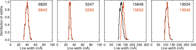
Figure 10: Distribution of line widths in the four line pairs across the cube after the Stokes profiles are spectrally and spatially degraded.

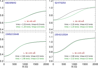
Figure 11: Calibration curves for the four line pairs shown for sample line widths indicated by L.W. The black and the green curves are with and without a macro-turbulent velocity of 2 km/s. In the green curves, the micro-turbulent velocity is reduced, to get the same line width.

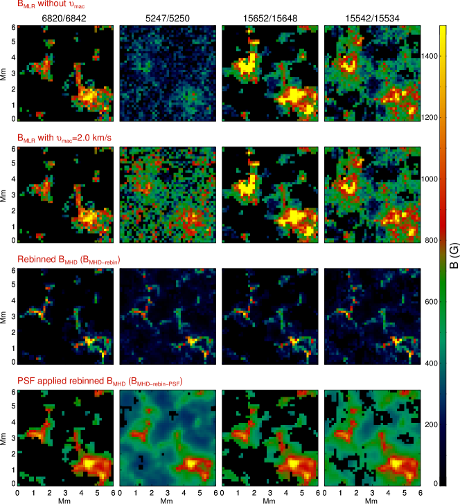
Figure 12: $B_{\rm MLR}$ determined from spatially and spectrally degraded Stokes $V$ profiles affected by noise, using calibration curves without macro-turbulent velocity (top row), and with a macro-turbulent velocity of 2.0 km/s (second row). This is compared with the magnetic field strength $B_{\rm MHD}$ re-binned according to Equation 3 ($B_{\rm MHD-rebin}$, third row). We show an empirical approximation of the result of MLR, based on $B_{\rm MHD-rebin}$ and including the influence of the PSF in the fourth row Note that all profiles have been broadened with a micro-turbulence to match the widths of the profiles emerging from the MHD snapshot.

To simulate the solar observations, we apply both spatial and spectral degradation to the Stokes profiles from the MHD cube and then estimate the $B_{\rm MLR}$. For this, the synthesized Stokes profiles are convolved with the theoretical point spread function (PSF) of the GREGOR telescope which includes the effects of spatial stray light. The profiles are then spectrally degraded by convolving them with a Gaussian with FWHM=30 mÅ and 100 mÅ respectively for the visible and IR line pairs. Later, they are re-binned to a detector pixel resolution of $0\arcsec.2$. For further details on the PSF used, see Lagg et al. (2016).

In addition to the degradation, we add a random noise of $\sigma=1\times 10^{-3}$ in the units of continuum intensity of the respective pair. We then consider all profiles with an amplitude larger than $3\sigma$ and apply a median filter over three wavelength pixels to smoothen the Stokes profiles. This threshold is applied to the magnetically weaker of the two lines in the pair. After spectral degradation and filtering, the Stokes profiles are further broadened. Hence we must construct new set of calibration curves for the four pairs. Repeating the same procedure as before, we plot the histograms of the line widths over the whole cube, in Figure 10. The line widths of the profiles are grouped into bins of 3 mÅ and 10 mÅ for the visible and IR pairs, respectively. At first, only $\varv_{\rm mic}$ is varied to match the line widths while keeping $\varv_{\rm mac}=0$, and the calibration curves are constructed. The effects of $\varv_{\rm mac}$ will be discussed later in the section.

The MLR estimates $B$ within the resolution element irrespective of the filling factor. In other words, in a resolution element containing a mix of magnetic and nonmagnetic components or strong and weak magnetic components, the MLR measures $B$ mainly from the strong magnetic component in the element and not the spatially averaged $B$ (Stenflo 1973). Hence, to compare with the fields in the MHD cube, we weight $B$ with the $V$ amplitude. By doing so, we give more weight to the magnetic field at locations where the Stokes V profile is stronger. In general these are the stronger magnetic fields (aligned along the line of sight), while the weaker (or more transverse) fields provide a proportionally smaller contribution to the line ratio. When such a weighted magnetic field strength is averaged to match the degraded pixel resolution, the resulting field strength has contributions mainly from the stronger magnetic component and resemble the field strength measured by MLR. Below we give an empirical relation aiming to provide a magnetic parameter that approximates the field strength sampled by the line ratio technique in the presence of finite spatial resolution. We call the magnetic field computed using this relation as $B_{\rm MHD-rebin}$. It is given by

$${B_{\rm MHD-rebin}(x^{\prime}_{p},y^{\prime}_{q})}\ {=}\ {\frac{\sum\limits_{j=aq}^{a(j+1)-1}\sum\limits_{i=ap}^{a(i+1)-1}[B_{\rm MHD}(x_{i},y_{j})V(x_{i},y_{j})]}{\sum\limits_{j=aq}^{a(j+1)-1}\sum\limits_{i=ap}^{a(i+1)-1}[V(x_{i},y_{j})]}},$$ (3)

where $p=0,1,..,m-1$; $q=0,1,..,n-1$, and the summations rebin the quantities in the square brackets. For the present purposes, the rebinning is done over 7 pixels, i.e. $a=7$, to match a detector pixel resolution of $0\arcsec.2$. The dimensions of $B_{\rm MHD-rebin}(x^{\prime},y^{\prime})$ is $(m,n)$. In the above equation, $B_{\rm MHD}(x,y)$ is computed from Equations (1) and (2) . $V(x,y)$ is the amplitude of the Stokes $V$ profile at pixel $(x,y)$ from the MHD cube at full resolution. When the fields are weak, $V\propto B$ and from Equation 3, $B_{\rm MHD-rebin}$ is $B_{\rm MHD}$ averaged over the resolution element.

Figure 12 shows a comparison between the $B_{\rm MLR}$ from the spatially and spectrally degraded profiles with $B_{\rm MHD-rebin}$ defined in Equation 3. In the first row the $B_{\rm MLR}$ is computed from the calibration curves which are constructed by varying only $\varv_{\rm mic}$ to match the line widths. The maps in the second row will be discussed later. The third row shows the magnetic field maps resulting from Equation 3. The shapes of the magnetic field structures from the MLR method in the first row do not resemble those in the third row. This is because the magnetic field structures in the first row, which are obtained by applying the MLR method on the PSF convolved Stokes $V$ profiles, are smeared out. This effect has not been accounted for, in Equation 3. In order to reproduce this effect, we apply the PSF to $B_{\rm MHD-rebin}$, to get $B_{\rm MHD-rebin-PSF}$. We stress that there is no clearcut physically consistent manner in which $B_{\rm MHD-rebin}$ can be convolved with the PSF. Our aim here is to empirically get a better idea of what quantity the MLR actually returns in a realistic atmosphere in the presence of spatial smearing. To that end we tried different things and compared the resulting maps with the first row of Figure 12. We found that the best agreement (in the shape of the features) was obtained by

$$B_{\rm MHD-rebin-PSF}(x^{\prime},y^{\prime}) = {\rm PSF}(x^{\prime},y^{\prime})\ \ast\ B_{\rm MHD-rebin}(x^{\prime},y^{\prime}),$$ (4)

where $B_{\rm MHD-rebin}(x^{\prime},y^{\prime})$ is defined in Equation 3 and $\ast$ represents convolution. After applying the PSF, however, the magnetic field is smeared and diluted (Lagg et al. 2016). Thus $B_{\rm MHD-rebin-PSF}$ is much smaller than $B_{\rm MHD-rebin}$ (third row of Figure 12). In the presence of spatial smearing, though result from MLR is spatially smeared, the strength of the field is maintained (i.e. still the intrinsic field strength is reached at the centers of magnetic features) and thus the $B_{\rm MHD-rebin-PSF}$ from Equation 4 is smaller also than the MLR results shown in the top row of Figure 12. Hence we normalize $B_{\rm MHD-rebin-PSF}$, such that its maximum field strength matches with the maximum of $B_{\rm MHD-rebin}$. In the fourth row we show maps of the normalized $B_{\rm MHD-rebin-PSF}$ and the pixels where the degraded Stokes $V$ is smaller than 3$\sigma$ are filtered out. Now the field structures in the first row resemble those in the fourth row.

The $B_{\rm MHD}$ in Equation 3 is obtained after weighting the original field in the MHD cube with the response function and integrating over tau, from Equations 1 and 2. Therefore, the original intrinsic field strength in the MHD cube is maintained. With Equations 3 and 4, we are trying to empirically represent the quantity that MLR method provides in a realistic atmosphere and for realistic instrumental degradation. This is not straightforward and has not been reported in the literature. By comparing the maps in the first and the fourth rows in Figure 12, we see that this empirical representation provides a reasonably close match with $B_{\rm MLR}$.

Due to smaller $V$ amplitudes in the 6842 Å line pair and the $1.56\,\mu$m line pair, about 30–45% of the profiles are above the $3\sigma$ threshold. As the lines in the 5250 Å pair and the $1.55\,\mu$m pair are stronger, more than 80% of the profiles remain above the $3\sigma$ level. The 6842 Å pair and the two IR pairs clearly show the presence of kG fields in the cube. But they are spread over larger areas because of the convolution with the PSF. The green patches surrounding the strong field yellow patches are due to redistribution of the photons caused by the PSF. This is also discussed in detail by Lagg et al. (2016).

The 5250 Å line pair, however, does not measure kG fields in the cube (first row in Figure 12). From this line pair, kG fields were not recovered also by Khomenko & Collados (2007) in an MHD cube and by Socas-Navarro et al. (2008) in solar network observations. In the former paper, the authors explained this to be due to the larger formation heights of the lines in the 5250 Å pair and that they sample weaker magnetic fields in the MHD cube. As kG fields could not be recovered in the network observations by Socas-Navarro et al. (2008), they concluded this line pair to be unreliable and that it is no better than the 6300 Å pair in which the two lines are formed at very different heights in the atmosphere. This is surprising because, the presence of kG fields in the solar network regions was discovered by applying MLR to the 5250 Å line pair by Stenflo (1973).

To investigate this, we included a constant height-independent $\varv_{\rm mac}$ of 2 km/s in addition to $v_{\rm mic}$ and recomputed the calibration curves. The $\varv_{\rm mic}$ was varied to get the required line widths. Examples comparing the calibration curves with and without $\varv_{\rm mac}$ for fixed line widths is shown in Figure 11. The 5250 Å line pair is the most affected by the addition of $\varv_{\rm mac}$. This pair is highly sensitive to both $\varv_{\rm mic}$ and $\varv_{\rm mac}$, as pointed out in Solanki et al. (1987); Khomenko & Collados (2007). The magnetic field strengths recovered from the new calibration curves are shown in the second row of Figure 12. The 5250 Å pair now shows the presence of kG fields in the cube. However, the magnetic field map from this line pair does not match well with those in the fourth row. This could be because of the approximations in the construction of the calibration curves. If the curves are constructed at every pixel by fitting the full spectral line then the 5250 Å pair may provide a better comparison with the magnetic field maps in the fourth row. The results from the other three line pairs are not much affected by the addition of $\varv_{\rm mac}$, as also seen from Figure 11. What we have presented is only a simplified approach, so that, if the 5250 Å line pair is to be used for MLR, both $\varv_{\rm mic}$ and $\varv_{\rm mac}$ should be varied to match the line width and depth at every pixel in the cube. In any case, the 5250 line pair is less robust than the others.

6 Conclusions

The magnetic line ratio (MLR) method has been widely used to measure magnetic field strengths on the Sun. Until recently, three line pairs (5250 Å, 6300 Å and $1.56\,\mu$m pairs) were used for this method, only two of which (5250 Å and $1.56\,\mu$m pairs) give reliable results. In this paper, we have identified two new line pairs, the 6842 Å pair in the visible and the $1.55\,\mu$m pair in the IR. Lines in the 6842 Å pair are separated by 22 Å and those in the new $1.55\,\mu$m pair by 8 Å. Lines in each of these pairs are formed at roughly the same height in the atmosphere. The new pairs have one line with high g_eff and with large difference in g_eff between the lines, making them well suited for MLR. We have presented a detailed comparison of the new and the old line pairs.

The Stokes profiles are synthesized in a three dimensional MHD cube having a field strength $B_{\rm MHD}$ (which differs from one pixel to the next). The MLR method is applied to the synthesized profiles to recover the field strengths, called $B_{\rm MLR}$. The $B_{\rm MLR}$ compares well when the $B_{\rm MHD}$ is weighted with the Stokes $V$ response function and then integrated over the optical depth grid. All the four line pairs reproduce $B_{\rm MHD}$, but the scatter in histogram of the difference between $B_{\rm MHD}$ and $B_{\rm MLR}$ is smaller for the new visible and IR pairs. The two lines in the new IR pair are stronger than the lines in the old $1.56\,\mu$m pair. Though the lines in new IR pair have Stokes $V$ signals that are typically smaller than the 15648 Å line (g${}_{\rm eff}=3$ line), they are much stronger than those of the g_eff= 1.53 line at 15652 Å line, used together with $\lambda$ 15648 Å. Thus, in the presence of noise, the Stokes profiles of both lines in the new $1.55\,\mu$m pair will remain above noise more often than the $1.56\,\mu$m pair, making them favourable also for the inversions.

We have further tested the line pairs by applying spatial and spectral degradation, and by adding random noise ($\sigma=1\times 10^{-3}I_{c}$) to the Stokes profiles. We find that the new 6842 Å pair and the old $1.56\,\mu$m pair are most affected by noise. However, more than 80% of the Stokes $V$ profiles from the new IR pair, remain above the $3\sigma$ cutoff.

Using the 5250 Å line pair, Khomenko & Collados (2007) and Socas-Navarro et al. (2008) could not recover kG fields from the profiles synthesized in a 3D MHD cube and in the solar network observations, respectively. While Khomenko & Collados (2007) attributed this to the larger formation heights of the lines in the 5250 Å pair, Socas-Navarro et al. (2008) concluded this line pair to be unreliable. We find that the 5250 Å pair is more sensitive to the nature of the velocity field, e.g. the exact mixture of micro and macro-turbulent velocities, than the other line pairs. Also, since the lines in this pair are strong and temperature sensitive, it is necessary to match the full line shape (line width and line depth) in the construction of calibration curves. From the calibration curves with the right combination of micro and macro-turbulent velocities, it is possible to measure kG fields from the 5250 Å pair. For the other three line pairs (6842 Å, old $1.56\,\mu$m and new $1.55\,\mu$m pairs), calibration curves constructed by matching the line widths is sufficient for measuring reliable magnetic field strengths.

The interpretation of the MLR has in the past been generally given in terms of an idealized 2-component atmosphere, a field free and a homogeneous magnetic component (Stenflo 1973). In this representation the field strength returned by the MLR is an approximation of the intrinsic field strength in the magnetic component. What happens in a more realistic, complex atmosphere with a distribution of field strengths and the influence of a PSF? Here it turns out that the MLR still gives an approximation of the intrinsic field strength at the average formation height of the Stokes $V$ lobes, but weighted by the amplitude of the Stokes $V$ profile (regions with small Stokes $V$ provide a smaller contribution). Also the influence of spatial smearing turns out to be complex. Ours is the first attempt to empirically determine what exactly the MLR returns in a realistic atmosphere. It can likely be improved.

Sophisticated inversion codes are currently the preferred choice for magnetic field measurements. We expect the new line pairs to be attractive pairs also for the application of inversion codes. In addition, it may be possible to combine the MLR with the inversions. One way would be to use the magnetic field strength measured from MLR as an initial guess in the inversions. Another is to employ the MLR as an additional constraint on the inversion. This will be investigated in a forthcoming paper.

Appendix A Anomalous Zeeman splitting and MLR

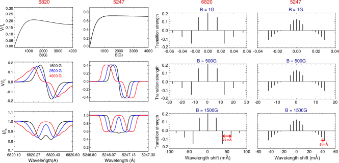
Figure 13: Variation in Stokes $V$ amplitude for the 6820 Å and 5247 Å lines as a function of magnetic field strength ($B$). Full line profiles are shown for 1.5, 2.5 and 4 kG. A comparison between the Zeeman splitting pattern for the two lines for $B$= 1, 500 and 1500 G is shown in the last two columns. Note the change in the wavelength scale of these plots with $B$.

In the presence of strong magnetic fields, the Zeeman saturation suppresses the amplitude of a Stokes $V$ profile and broadens its lobes. In normal Zeeman triplets, as $B$ increases, the amplitude of Stokes $V$ increases until it saturates. For field strengths beyond that, it remains constant. When the Zeeman splitting is anomalous, Stokes $V$ continues to change with $B$ (Solanki 1993). In the new line pairs, the 6820 Å and 15534 Å lines undergo anomalous Zeeman splitting. For stronger fields, their Stokes $V$ amplitudes decrease when $B$ exceeds a certain threshold value, $B_{\rm th}$.

The 5247 Å line is also not a normal Zeeman triplet, but its Stokes $V$ begins to decrease significantly only when $B$ exceeds 5 kG. A comparison between the 6820 Å and the 5247 Å lines is shown in Figure 13. The behaviour of the Stokes $V$ amplitude is governed by the splitting of the individual transitions forming a given $\sigma$-component. For $B=1.5$ kG, the separation between the various transitions in a $\sigma$-component ($\Delta\lambda_{B}$) in the 6820 Å line is as high as 22 mÅ, whereas in the 5247 Å line it is only 5 mÅ (indicated with red arrows in Figure 13). As $B$ increases, $\Delta\lambda_{B}$ becomes comparable to the line widths of the individual transitions, resulting in broadening of the $\sigma$-component and a corresponding decrease of the $V$ amplitude. This is clear when $B$ is increased to 4  kG, we see peaks of the line profiles from each transition in the 6820 Å line (first column in Figure 13) but not in the 5247 Å line (second column in Figure 13).

The $\Delta\lambda_{B}$ for a Zeeman component ($\pi$ or $\sigma$) is proportional to ($m_{l}$ g${}_{l}\,-\,m_{u}$ g_u) where $m_{l,u}$ are the magnetic quantum numbers of the lower and upper levels of the transition, respectively. The Landé g-factors of the upper and lower atomic levels are denoted as g_u and g_l, respectively. For the $\sigma$ components, $\delta m=(m_{u}\,-\,m_{l})$ is $\pm 1$ and hence $\Delta\lambda_{B}\propto m_{u}($g${}_{l}\,-\,$g${}_{u})\ \pm\$g_l (del Toro Iniesta 2007). For the 6820 Å line, $\Delta\lambda_{B}$ is much larger with $\delta$g =—g${}_{l}\,-\,$g_u—= 0.67 and g_l=2.5 compared to the 5247 Å line, with $\delta$g = 0.25 and g_l=0.5. The $\Delta\lambda_{B}$ is large also for the 15534 Å line with $\delta$g = 0.33 and g_l=1.5. If g_l = 0 or g_u = 0 or $\delta$g = 0 then it is a normal Zeeman triplet and there is no change in $V$ amplitude after Zeeman saturation. The calibration curves for MLR for line pairs having at least one line which undergoes anomalous Zeeman splitting do not saturate, that is, reach a constant value for stronger fields. Depending on whether the line with anomalous splitting is the magnetically weaker or the stronger in the pair, the calibration curve, when computed as the ratio of magnetically weaker to the stronger line, either decreases (6842 Å pair) or increases (1.55 $\mu$m pair) with $B$ as seen from Figure 8.

The profiles in Figure 13 are computed without $\varv_{\rm mac}$ and $\varv_{\rm mic}$. Velocity broadening increases the value of $B_{\rm th}$ at which Stokes $V$ starts to decrease (see Figure 8). This behaviour, however, does not affect the diagnostic potential of the new line pairs as long as the line broadening is properly taken into account (which can easily be done by fitting the observed line profile).