Delay-time distribution in the scattering of time-narrow wave packets (II) - Quantum Graphs

Abstract

We apply the framework developed in the preceding paper in this series [1] to compute the time-delay distribution in the scattering of ultra short RF pulses on complex networks of transmission lines which are modeled by metric (quantum) graphs. We consider wave packets which are centered at high quantum number and comprise many energy levels. In the limit of pulses of very short duration we compute upper and lower bounds to the actual time delay distribution of the radiation emerging from the network using a simplified problem where time is replaced by the discrete count of vertex-scattering events. The classical limit of the time-delay distribution is also discussed and we show that for finite networks it decays exponentially, with a decay constant which depends on the graph connectivity and the distribution of its edge lengths. We illustrate and apply our theory to a simple model graph where an algebraic decay of the quantum time delay distribution is established.

1 Introduction

1.1 Motivations

When an ultra-short pulse of radiation is scattered on a complex medium, the emerging radiation pulse is broadened in time and the pulse shape reflects the distribution of time-delays induced in the scattering process. This distribution can be intuitively explained as due to the existence of a large number of paths of varying lengths through which the radiation can traverse the scatterer. Recently, novel methods to produce ultra-short light pulses were introduced. They opened a new horizon for experiments where the distribution of delay-times induced by scattering from complex targets can be measured, with interesting and surprising results, see e.g., [2, 3, 4]. The ultra-short pulses are realized as broad-band coherent wave packets, which are presently available only for electromagnetic radiation, but not yet for sub-atomic particles such as e.g., electrons. However, work towards this end has already begun [5]. These developments emphasize the need for theoretical tools to aid planning of new experiments and interpret the measured results.

The preceding paper in this series [1] presented a general theoretical framework for the computation of the delay-time distribution in scattering of short radiation pulses on complex targets. The ingredients which are needed in this theory are the scattering matrix $S(k)$ where $k$ is the wave-number, the pulse (wave-packet) envelope $\omega(k)$ and the dispersion relation $E(k)$. For scattering of electromagnetic radiation the latter is $E(k)=ck$ where $c$ denotes the velocity of light. In this case it is convenient to express the time by the optical path-length $s=tc$. The general expression for the delay-time distribution is then given by

$$P_{{f},{i}}(s)=\frac{1}{2\pi}\ \left|\int_{0}^{\infty}{\rm d}k\ \omega(k)S_{f,i}(k)e^{-iks}\right|^{2}$$ (1)

if the delay is measured for pulses impinging in channel $i$ and detected in channel $f$.

In the present paper, we apply this general formalism to scattering on quanum graphs [6, 7, 8, 9, 10]. We do so for two reasons: First, quantum graphs are known as a successful paradigm for scattering from complex targets while at same time they are analytically and numerically much more tractable. For example we will present in this paper a full analytic solution of a model which contains some essential ingredients for complex targets such as an exponetially increasing number of scattering trajectories and relevant quantum interferences between them. Thus, studying quantum graphs in the present context might reveal typical features which are difficult to decipher in more realistic systems. Second, quantum graphs are very good models for the scattering of radio frequency (RF) signals in networks of wave-guides. As a matter of fact, experiments on the delay-time distribution in such systems are presently performed in Maryland and Warsaw [11, 12].

1.2 Outline

In the following Section 1.3 the necessary definitions and tools from the theory of quantum graphs will be provided. Then in Section 1.4 this theory will be extended to scattering on graphs and an explicit formula for the scattering matrix $S_{f,i}$ will be discussed. In Section 2 we apply this formula to Eq. (1) and derive on this basis approximate expressions for the delay time distribution in the case of broad envelope functions $\omega(k)$ corresponding to wave packets narrow in time.

Section 3 is devoted to the clasical analogue of the delay time distribution. In particular we show that for finite and connected graphs the classical delay distribution decays exponentially for long times and calculate the decay exponent. The classical delay distribution provides both, a simple short-time approximation to the fully coherent expression (1) and a reference result which allows to highlight quantum interference contributions to (1) for longer times. Moreover, as in the above mentioned experiments with RF radiation some decoherence cannot be avoided, a satisfactory theory might involve a crossover between our results for coherent and incoherent time delay.

In the final Section 4 we apply all our results to a simple model system which consists of two edges and a single scattering channel. For this model we can also confirm the results of Section 2 by an independent calculation based on the distribution of narrow scattering resonances.

1.3 Quantum graphs in a nut-shell

A graph $\mathcal{G}(\mathcal{V,E})$ consists of a finite set of vertices $\mathcal{V},\ |\mathcal{V}|=V$ and edges $\mathcal{E},\ |\mathcal{E}|=E$. It will be assumed that $\mathcal{G}$ is connected and simple (no parallel edges and no self connecting loops). The connectivity of $\mathcal{G}$ is encoded in the $V\times V$ adjacency matrix $A$: $A_{u,v}=1$ if the vertices $u,v\in\mathcal{V}$ are connected and $A_{u,v}=0$ otherwise. The set of edges connected to the vertex $v$ is denoted by $\mathcal{S}(v)$. The degree of the vertex $v$ is $d_{v}=|\mathcal{S}(v)|$. When $A_{u,v}=1$, the connecting edge $e=(u,v)$ will be endowed with two directions $\varpi=\pm$, the positive direction is chosen to point from the lower indexed vertex to the higher. A pair $d=(e,\varpi)$ is a directed edge. The set of all directed edges will be denoted by $\mathcal{D}$ and $D=|\mathcal{D}|=2E$ is its size. The reverse of $d$ is denoted by ${\hat{d}}=(e,-\varpi)$. When $d$ is a directed edge pointing from vertex $u$ (the origin of $d$) to $v$ (the terminus of $d$) we write $u=o(d)$ and $v=t(d)$, respectively.

An alternative way to describe the connectivity of $\mathcal{G}$ is in terms of the edge adjacency matrix of dimension $D\times D$ :

$$B_{d,d^{\prime}}=\delta_{o(d),t(d^{\prime})}\ ,\ \ d,d^{\prime}\in\mathcal{D}\ .$$ (2)

The metric endowed to the graph is the natural one-dimensional Euclidian metric on every edge. The length of an edge $e$ is denoted by $L_{e}$ and $\mathcal{L}=[L_{e}]_{e=1}^{E}$ is the set of these edge lengths. The edge lengths $L_{e}$ are assumed to be rationally independent. A graph is compact when all the edge lengths $L_{e}$ are finite. The lengths of the directed edges $d$ and its reverse $\hat{d}$ are equal. Denote by $x_{e}$ the coordinate of a point on the edge $e$, measured from the vertex with the smaller index and $0\leq x_{e}\leq L_{e}$. A function $F:x\in\mathcal{G}\rightarrow\mathbb{R}$ is given in terms the functions $[f_{e}(x_{e})]_{e=1}^{E}$ so that if $x\in e,\ F(x)=f_{e}(x)$. The action of the Laplacian on $F(x)$ for $x\in e$ is $\Delta_{\mathcal{G}}F=-\frac{\partial^{2}f_{e}}{\partial x_{e}^{2}}$ and the domain of the Laplacian is $f_{e}({x_{e}})\in\mathcal{C}^{2}(0,L_{e}),\ \forall e$. Assume $\mathcal{G}$ is compact. Then, the Laplacian is self-adjoint if it acts on a restricted space of functions $F(x)$ which satisfy appropriate boundary conditions. Frequently used boundary conditions are the Neumann conditions which require the function $F$ to be continuous at all the vertices, and for every vertex, $\sum_{e\in\mathcal{S}(v)}\frac{\partial f_{e}(x_{e})}{\partial x_{e}}|_{v}=0$, where the derivatives at $v$ are taken in the direction which points away from $v$. The most general prescriptions for boundary conditions were first introduced and discussed in [13]. The time dependent wave equation (with time $s/c$) is

$$\frac{\partial^{2}\ }{\partial s^{2}}F(x,s)=\Delta_{\mathcal{G}}F(x,s)$$ (3)

with the boundary conditions specified above which must be satisfied for all $s$. The stationary equation

$$\Delta_{\mathcal{G}}F(x,k)=k^{2}F(x,k)\ ,$$ (4)

can be solved only for a discrete, yet infinite set of wave numbers $[k_{n}]_{n\in\mathbb{Z}}$ which is the spectrum of the stationary wave equation.

A useful method of computing the spectrum of the graph Laplacian is based on the following decomposition of the wave function. Consider the functions $f_{e}(x_{e})=a_{d}e^{i\varpi kx_{e}}+a_{\hat{d}}e^{i\varpi k(L_{e}-x_{e})}$, where $d=(e,\varpi)$ and $a_{d},a_{\hat{d}}$ are arbitrary complex numbers. These functions are the general solutions of $-\frac{\partial^{2}f_{e}}{\partial x_{e}^{2}}=k^{2}f_{e}(x_{e})$ on all the edges. The constants should be computed so that $F(x)$ satisfies the boundary conditions at all the vertices. Consider all the edges which are connected to a vertex $v:\ e\in\mathcal{S}(v)$. For Neumann boundary conditions the continuity of the graph wave function at the vertex $v$ imposes $d_{v}-1$ independent requirements on the coefficients $a_{d}$. Namely, $f_{e}|_{v}=f_{e^{\prime}}|_{v}\forall e\neq e^{\prime}\in{\mathcal{S}(v)}$, where $f_{e}|_{v}$ denotes the value of $f_{e}$ at the vertex $v$, where $x_{e}=0$ or $x_{e}=L_{e}$ depending on the orientation of $d$. Again for Neumann boundary conditions, another relation among the $a_{d}$ is imposed by the requirement that the sum of the outgoing derivatives of the $f_{e}$ at the vertex vanishes. Therefore there are $d_{v}$ linear equations which the $2d_{v}$ coefficients must satisfy. Hence, if one denotes the set of directed edges which point towards $v$ by $\mathcal{S}^{-}(v)$ and the complementary set of outgoing directed edges by $\mathcal{S}^{+}(v)$, then the boundary conditions at $v$ provide a linear relation between the two subsets of coefficients:

$$a_{d}=\sum_{d^{\prime}\in\mathcal{S}^{-}(v)}\sigma^{(v)}_{d,d^{\prime}}a_{d^{\prime}},\ \ \ \forall d\in\mathcal{S}^{+}(v)\ ,\ \ \ {\rm with}\ \ \sigma^{(v)}_{d,d^{\prime}}=\frac{2}{d_{v}}-\delta_{d,{\hat{d}}^{\prime}}\ .$$ (5)

The symmetric and unitary matrix $\sigma^{(v)}$ of dimension $d_{v}$ is the vertex scattering matrix corresponding to Neumann boundary condition at the vertex. Other boundary conditions yield different vertex scattering matrices, and their unitarity is due to the fact that the underlying graph Laplacian is self adjoint. Using the vertex scattering matrices for all the vertices on the graph, one can construct a $D\times D$ unitary matrix

$$U_{d,d^{\prime}}(k)=\delta_{o(d),t(d^{\prime})}e^{ikL_{d}}\sigma^{(o(d))}_{d,d^{\prime}}\ ,\ d,d^{\prime}\in\mathcal{D}\ ,$$ (6)

which acts on the $D$ dimensional space of complex coefficients $a_{d}$. It then follows [6, 7] that the spectrum of the graph Laplacian is obtained for values of $k$ which satisfy the secular equation

$$\det[I^{(D)}-U(k)]\ =\ 0\ ,$$ (7)

where $I^{(D)}$ is the unit matrix in dimension $D$. The unitarity of $U(k)$ for real $k$ implies that all the eigenvalues of $U(k)$ are on the unit circle. As $k$ varies, eigenvalues cross the real axis, where the secular equation is satisfied. Therefore the $k$ spectrum is real.

$U(k)$ is referred to as the graph evolution operator in the quantum chaos literature. Its matrix elements provide the amplitudes for scattering from an edge $d$ directed to a vertex $v$, to an edge $d^{\prime}$ directed away from $v$. Their absolute squares can be interpreted as the probabilities that a classical particle confined to the graph and moving on the edge $d$ toward the vertex $v$ is scattered to the edge $d^{\prime}$ and moves away from it. Due to the unitarity of $U$ the $D\times D$ matrix $M$

$$M_{d,d^{\prime}}=|U_{d,d^{\prime}}|^{2}\ ,\ \ d,d^{\prime}\in\mathcal{D}\ ,$$ (8)

does not depend on $k$ and is double Markovian: $\sum_{d}M_{d,d^{\prime}}=\sum_{d^{\prime}}M_{d,d^{\prime}}=1$. The transition probability matrix $M$ allows to define a random walk on the graph. For the graphs considered here, $M$ satisfies the conditions of the Frobenius-Perron theorem and therefore the largest eigenvalue of $M$ is $1$ and it is single. Suppose that at time $0$ the probability distribution to find the walker on the directed edge $d$ is given by the vector $p_{d}(t=0),\ \forall d\in\mathcal{D}$. Then, at integer time $t>0$ the distribution will be $p(t)=M^{t}p(0)$ and converges to equidistribution for large $t$ independently of the initial probability distribution. In other words, the classical evolution on the graph is ergodic. (Note that we will use the symbol $t$ for a discretized topological time while the continuous physical time is measured in terms of the path length $s$ as in Eq. (1).)

1.4 Scattering on quantum graphs

So far we discussed the wave equation and its classical limit on a compact graph. To turn this graph into a scattering system, we choose a subset of vertices $\mathcal{H}\in\mathcal{V}$, and at every vertex $h\in\mathcal{H}$ we add a semi-infinite edge (lead). $H=|\mathcal{H}|$ is the number of leads. The directed edges on the lead attached to vertex $h$ are denoted by $h^{(+)}$ which points away from the vertex $h$ and $h^{(-)}$ which points towards it. The Laplacian is extended to the leads in a natural way, and the boundary conditions at the vertices $h\in\mathcal{H}$ are modified by replacing $d_{v}$ by $d_{h}=d_{v}+1$. Measuring distances from the vertex $h$ outwards, the functions which are allowed on the lead take the form $f_{h}(x)=a_{h^{(-)}}e^{-ikx}+a_{h^{(+)}}e^{ikx}$. The spectrum of the Laplacian for a scattering graph is continuous and covers the entire real line, possibly with a discrete set of embedded eigenvalues (See e.g., [10]).

Consider the matrix

$$W_{d,d^{\prime}}=\delta_{o(d),t(d^{\prime})}e^{ikL_{d}}{\tilde{\sigma}}^{(o(d))}_{d,d^{\prime}}\ ,\ \ d,d^{\prime}\in\mathcal{D}\ ,$$ (9)

where ${\tilde{\sigma}}^{(u)}$ for $u\in\mathcal{H}$ are the vertex scattering matrices which are modified as explained above, and for $u$ in the complement of $\mathcal{H}$, they take the values of the vertex scattering matrices for the compact graph. Note that $W(k)$ is a $D\times D$ matrix, and its entries are indexed by the labels of the directed edges in the compact part of the graph, in the same way as the original matrix $U(k)$ of Eq. (6). However, unlike $U(k)$, $W(k)$ is not unitary, because some of its building blocks, namely the vertex scattering matrices ${\tilde{\sigma}}^{(h)},h\in\mathcal{H}$ are not unitary when they are restricted to the directed edges in the compact part of the graph.

The analogue of $M$ defined in (8) for the non-compact graph is

$${\tilde{M}}_{d,d^{\prime}}=|W_{d,d^{\prime}}|^{2}=\delta_{o(d),t(d^{\prime})}\left|{\tilde{\sigma}}^{(o(d))}_{d,d^{\prime}}\right|^{2}\ .$$ (10)

It is independent of $k$ and sub-Markovian since for $o(d)\in\mathcal{H}$ the sums $\sum_{d^{\prime}}{\tilde{M}}_{d,d^{\prime}}$ and $\sum_{d^{\prime}}{\tilde{M}}_{d^{\prime},d}$ are strictly less than $1$. The Perron-Frobenius theorem guarantees that the spectrum of $\tilde{M}$ is confined to the interior of the unit circle. For a random walker whose evolution is dictated by $\tilde{M}$, the probability to stay inside the compact part of the graph approaches zero after sufficiently long time. This is due to the walks which escape to the leads and never return.

Consider now a solution of the stationary wave equation for a given $k$ subject to the condition that the wave function on the leads has the form $f_{h}(x_{h})=a_{h^{(-)}}e^{-ikx_{h}}+a_{h^{(+)}}e^{+ikx_{h}}$. The scattering matrix for a non compact graph is a unitary matrix of dimension $H$ which provides the vector of ”outgoing amplitudes” ${\bf a}^{(+)}=\{a_{h^{(+)}}\}_{h\in H}$ in terms of the vector of ”incoming amplitudes” ${\bf a}^{(-)}=\{a_{h^{(-)}}\}_{h\in H}$. It follows from the linearity of the wave equation that

$${\bf a}^{(+)}=S(k){\bf a}^{(-)}\ .$$ (11)

The explicit expression for $S(k)$ was derived in [14, 10] and will be quoted here without proof:

$$S_{h,h^{\prime}}(k) =\delta_{h,\hat{h}^{\prime}}\rho_{h^{\prime}}+\sum_{d,d^{\prime}}\tau_{h,d}\left\{\sum_{n=0}^{\infty}[W^{n}(k)]_{d,d^{\prime}}\right\}\ e^{ikL_{d^{\prime}}}\tau_{d^{\prime},h^{\prime}}$$

$$=\delta_{h,\hat{h}^{\prime}}\rho_{h^{\prime}}+\sum_{d,d^{\prime}}\tau_{h,d}\left[I^{(D)}-W(k)\right]^{-1}_{d,d^{\prime}}\ e^{ikL_{d^{\prime}}}\tau_{d^{\prime},h^{\prime}}\ .$$ (12)

Here, $\rho_{h}={\tilde{\sigma}}^{(h)}_{{\hat{h}},h}$ is the back reflection amplitude, $\tau_{d^{\prime},h^{\prime}}={\tilde{\sigma}}^{(h^{\prime})}_{d^{\prime},h^{\prime}}$ is the transmission amplitude from the lead $h^{\prime}$ to the edge $d^{\prime}$ in the compact part of the graph, and $\tau_{h,d}$ is the transmission amplitude from an edge $d$ in the compact graph to a lead $h$. The first line in (1.4) expresses the fact that scattering proceeds by either reflecting from the incoming lead back to itself (the term outside the sum), or by penetrating to the compact part and scattering inside it several times before emerging outside. The contribution of the scattering process in the compact graph is provided by the expression in curly brackets. It can be rewritten as

$$\sum_{d,d^{\prime}}\tau_{h,d}\left\{\sum_{n=0}^{\infty}[W^{n}(k)]_{d,d^{\prime}}\right\}\ e^{ikL_{d^{\prime}}}\tau_{d^{\prime},h^{\prime}}=\sum_{n=0}^{\infty}\sum_{\alpha\in{\mathcal{A}}_{h,h^{\prime}}^{(n)}}A^{(n)}_{\alpha}e^{ikl_{\alpha}}.$$ (13)

Here, $n$ counts the number of vertices on a path $\alpha$ connecting the entrance and exit vertices $h^{\prime}$ and $h$. ${\mathcal{A}}^{(n)}_{h,h^{\prime}}$ is the set of all the paths crossing $n$ vertices which start on $h^{\prime}$ and end at $h$ after traversing $n+1$ directed edges $(d_{0},d_{1},\cdots,d_{n}),d_{j}\in\mathcal{D}$ with $o(d_{0})=h^{\prime},t(d_{n})=h$. Each path is of length $l_{\alpha}=\sum_{j=0}^{n}L_{d_{j}}$. The term $n=0$ occurs only when $h^{\prime}$ and $h$ are neighbors on $\mathcal{G}$. Then $\alpha$ is the directed edge $d$ connecting $h^{\prime}$ to $h$, $\mathcal{A}_{h,h^{\prime}}^{(0)}$ consists of the single bond $d$, $A^{(0)}=\delta_{d,d^{\prime}}\tau_{h,d}\tau_{d,h^{\prime}}$ and $l_{\alpha}=L_{d}$. For $n\geq 1$ the amplitudes $A_{\alpha}^{(n)}$ can be written as

$$A_{\alpha}^{(n)}=\tau_{h,d_{n}}\left[\prod_{j=1}^{n}\sigma^{(o(d_{j}))}_{d_{j},d_{j-1}}\right]\tau_{d^{\prime},h^{\prime}}\ .$$ (14)

The series in the first line of (1.4) converges to the expression in the second line for any real $k$ because $W(k)$ is sub-unitary. The explicit form of the $S(k)$ matrix provided in Eq. (1.4) will be used in the next sections. An alternative expression for $S(k)$ which will not be used here can be found in [7].

2 Scattering of wave-packets and the delay-time distribution

Given a graph with leads to infinity as defined above, we consider a particular solution of the stationary wave equation with wave number $k$, where the wave function consists of an incoming wave with unit amplitude in a single lead $h^{\prime}$ but outgoing waves in all the leads. Limiting our attention to a specific lead $h$ the wave function has the form

$$f_{h}(x_{h})=\delta_{h,h^{\prime}}e^{-ikx_{h}}+a_{h{{}^{(+)}}}e^{ikx_{h}}=\delta_{h,h^{\prime}}e^{-ikx_{h}}+S_{h,h^{\prime}}(k)e^{ikx_{h}}$$ (15)

The last equality follows from the definition of the scattering matrix. A time-dependent solution describing the propagation of a wave packet is obtained by a superposition of functions $f_{h}(x_{h})$ with an envelope function $\omega(k)$. As in [1] $\omega(k)$ is positive and normalized by $\int_{0}^{\infty}\omega^{2}(k){\rm d}k=1$. Assuming a linear dispersion relation (such as e.g. for electromagnetic waves in transmission lines), the intensity of the outgoing wave function in the position $x_{h}=0$ at time $s/c$ is

$$P_{h,h^{\prime}}(s)=\frac{1}{2\pi}\left|\int_{0}^{\infty}\omega(k)S_{h,h^{\prime}}(k)e^{-iks}{\rm d}k\ \right|^{2}\ ,$$ (16)

which is the analogue of equation (11) in [1]. The unitarity of $S$ guarantees the conservation of probability.

$$\sum_{h}\int_{-\infty}^{\infty}P_{h,h^{\prime}}(s){\rm d}s=1\ .$$

For a Gaussian envelope,

$$\omega(k)=\left(\frac{2}{\pi\sigma^{2}}\right)^{\frac{1}{4}}e^{-\frac{(k-k_{0})^{2}}{\sigma^{2}}}$$ (17)

and under the condition $k_{0}>2\sigma$, one can approximate the delay-time distribution by (see (17) in [1])

$$P_{h,h^{\prime}}(s) \approx \frac{1}{2\pi}\int_{-\infty}^{\infty}{\rm d}\eta\ e^{-i\eta s}e^{-\frac{\eta^{2}}{2\sigma^{2}}}\times$$ (18)

$$\left\{\sqrt{\frac{2}{\pi\sigma^{2}}}\int_{-\infty}^{\infty}{\rm d}\xi\ e^{-\frac{2(\xi-k_{0})^{2}}{\sigma^{2}}}S_{h,h^{\prime}}\left(\xi+\frac{\eta}{2}\right)\ \overline{S_{h,h^{\prime}}}\left(\xi-\frac{\eta}{2}\right)\right\}.$$

Using Eq. (13) one can write an explicit expression for $P_{h,h^{\prime}}(s)$ for any values of $\sigma$ and $k_{0}$ which satisfy the conditions underlying (18),

$$P_{h,h^{\prime}}(s) = \sum_{n=0}^{\infty}\sum_{\alpha,\beta\in\mathcal{A}^{(n)}_{h,h^{\prime}}}\left[e^{ik_{0}(l_{\alpha}-l_{\beta})}e^{-(l_{\alpha}-l_{\beta})^{2}\sigma^{2}/8}\right]A^{(n)}_{\alpha}\overline{A^{(n)}_{\beta}}\times$$ (19)

$$\left[\frac{\sigma}{\sqrt{2\pi}}e^{-\left(\frac{l_{\alpha}+l_{\beta}}{2}-s\right)^{2}\sigma^{2}/2}\right].$$

In the above result, we did not include the reflections from the vertex $h^{\prime}$ (which correspond to zero delay). To render the discussion more transparent, we shall proceed in the limit where $\sigma$ is very large, which allows to write the first square bracket above as a Kronecker $\delta$ and the last square bracket as a Dirac $\delta$ functions, resulting in

$$P_{h,h^{\prime}}(s)=\sum_{n=0}^{\infty}\sum_{\alpha,\beta\in\mathcal{A}^{(n)}_{h,h^{\prime}}}\delta_{l_{\alpha},l_{\beta}}A^{(n)}_{\alpha}\overline{A^{(n)}_{\beta}}\delta(l_{\alpha}-s)\ .$$ (20)

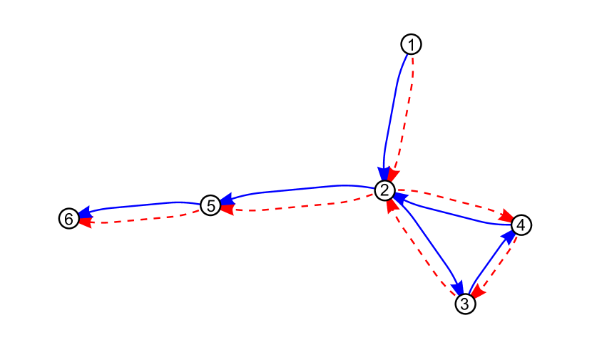
Figure 1: Isometric but topologically distinct paths differing in the orientation in which a loop of three vertices is traversed.

This expression can be simplified by recalling that the length of any path $\alpha\in\mathcal{A}_{h,h^{\prime}}^{(n)}$ can be written as $l_{\alpha}=\sum_{e\in\mathcal{E}}q_{e}(\alpha)L_{e}$ where $q_{e}$ are non negative integers whose sum is $n+1$. Note that $l_{\alpha}$ does not depend on the direction in which the edges are traversed. Because of the rational independence of the edge lengths, paths which share the same length must share also the same sequences $\{q_{e}\}_{e\in\mathcal{E}}$, and they are distinct if they cross the same edges the same number of times but in different order. Figure 1 shows an example for such isometric but topologically distinct paths. Denote ${\bf q}^{(n)}=\{q_{e}\}_{e\in\mathcal{E}}$ with $\sum q_{e\in\mathcal{E}}=n+1$. The set of isometric paths which share the code ${\bf q}^{(n)}$ will be denoted by $\Gamma_{h,h^{\prime}}({\bf q}^{(n)})$. Then

$$P_{h,h^{\prime}}(s) = \sum_{n=0}^{\infty}\sum_{{\bf q}^{(n)}}\left|\sum_{\gamma\in\Gamma_{h,h^{\prime}}({\bf q}^{(n)})}A^{(n)}_{\gamma}\right|^{2}\delta(l_{{\bf q}^{(n)}}-s)$$ (21)

$$= \sum_{n=0}^{\infty}\sum_{{\bf q}^{(n)}}p_{{\bf q}^{(n)}}\delta(l_{{\bf q}^{(n)}}-s)\ .$$ (22)

where the probabilities $p_{{\bf q}^{(n)}}$ contain all interference effects between the isometric paths belonging to $\Gamma_{h,h^{\prime}}({\bf q}^{(n)})$. The result of these interferences is determined by the phases of the individual amplitudes $A^{(n)}_{\gamma}$. These in turn depend on the phases of the elements of the vertex-scattering matrices $\sigma^{(v)}_{d_{j+1},d_{j}}$ encountered along the path $\gamma$ but they are independent of the precise values of the edge lengths. Thus, the only information about the actual lengths of the graph edges in the delay time distribution comes from the Dirac delta functions concentrating at the path lengths $l_{{\bf q}^{(n)}}=\sum_{e\in\mathcal{E}}q_{e}L_{e}$.

It is convenient to define the cumulative probability

$$C_{h,h^{\prime}}(s)=\int_{0}^{s}P_{h,h^{\prime}}(t){\rm d}t=\sum_{n=0}^{\infty}\sum_{{\bf q}^{(n)}}p_{{\bf q}^{(n)}}\Theta(s-l_{{\bf q}^{(n)}})\ ,$$ (23)

where $\Theta(x)$ is the Heavyside function. Clearly, $C_{h,h^{\prime}}(s)$ is a non-decreasing function of s. On the other hand it depends parametrically on the edge lengths $\mathcal{L}$ and is a non-increasing function of any $L_{e}\ (e\in\mathcal{E})$, because these lengths appear only in the arguments of the Heavyside step functions. We can use this fact to bound $C_{h,h^{\prime}}(s)$ from below and above by similar expressions with modified edge lengths. To this end define the function

$$C_{h,h^{\prime}}(s,\ell)=\sum_{n=0}^{\infty}\sum_{{\bf q}^{(n)}}p_{{\bf q}^{(n)}}\Theta(s-(n+1)\ell)\,,$$ (24)

where all edge lengths have been replaced by one and the same value $\ell$. Note that this is a formal definition and not related to the delay distribution of a graph with equal edge lengths, because Eq. (23) was derived under the assumption of rationally independent lengths. Take now $\ell=\max(L_{e})=\overline{L}$ being the maximum of the edge lengths of the graph under consideration. For the same value of $s$ the arguments of the Heavyside functions in Eq. (24) are smaller (or equal) in comparison to Eq. (23) and thus in Eq. (24) less terms contribute. Repeating this argument for $\min(L_{e})=\underline{L}$ we see that the cumulative delay distribution can be bound from below and above by

$$C_{h,h^{\prime}}(s;\overline{{L}})\leq C_{h,h^{\prime}}(s)\leq C_{h,h^{\prime}}(s;\underline{{L}})\ .$$ (25)

Note that $C_{h,h^{\prime}}(s;\ell)=C_{h,h^{\prime}}(s/\ell;1)$. Thus it suffices to calculate $C_{h,h^{\prime}}(t;1)$ for integer values of $t$. We refer to this quantity as the cumulative probability for the topological delay time $t$, i.e. the number of edges along the walk. Since there is no metric information to consider, $C_{h,h^{\prime}}(t;1)$ is typically easier to calculate than the full expression in Eq. (23).

To proceed, write $P_{h,h^{\prime}}(s)=P^{(D)}_{h,h^{\prime}}(s)+P^{(ND)}_{h,h^{\prime}}(s)$, where

$$P^{(D)}_{h,h^{\prime}}(s)=\sum_{n=0}^{\infty}\sum_{{\bf q}_{n}}\left[\sum_{\gamma\in\Gamma_{h,h^{\prime}}({\bf q}^{(n)})}|A^{(n)}_{\gamma}|^{2}\right]\delta(l_{{\bf q}^{(n)}}-s)$$ (26)

$$P^{(ND)}_{h,h^{\prime}}(s)=\sum_{n=0}^{\infty}\sum_{{\bf q}_{n}}\left[\sum_{\gamma\neq\gamma^{\prime}\in\Gamma_{h,h^{\prime}}({\bf q}^{(n)})}A^{(n)}_{\gamma}\overline{A^{(n)}_{\gamma^{\prime}}}\right]\delta(l_{{\bf q}^{(n)}}-s)\ .$$ (27)

The partition of the delay-time distribution into the Diagonal part $P^{(D)}_{h,h^{\prime}}(s)$ and the Non-Diagonal part $P^{(ND)}_{h,h^{\prime}}(s)$ separates the purely ”classical” contribution from the contribution from the interference of waves which propagate on isometric paths. The former will be studied in the next section. Sometimes, (when e.g., $h\neq h^{\prime}$ and the graph is not invariant under geometrical symmetries) the contribution of $P^{(ND)}_{h,h^{\prime}}(s)$ can be ignored upon further averaging. However this is not always the case, especially since the number of isometric trajectories $|\Gamma_{h,h^{\prime}}({\bf q}^{(n)})|$ may increase indefinitely with $n$ [15, 16, 17], and the sums do not necessarily vanish in spite of the fact that the individual contributions have complicated, seemingly random phases.

While some general properties of the classical time-delay distribution (26) can be derived as presented in the next section, there are no analogous results pertaining to the complete expression in Eq. (22). However, in section 4 we shall apply all results of the present and the following section to a simple graph and derive analytical results for both, the classical and the quantum delay distribution.

3 The classical delay-time distribution

In the present section we provide a classical description of the delay-time distribution. It is a valid approximation when quantum interference effects are negligible, either because of decoherence mechanisms in the scattering process or for short times, when the contributing trajectories do not have isometric partners. For long times and coherent dynamics a comparison to the reference provided by the classical description can highlight the features of the delay distribution which are due to genuine quantum (wave) properties of the scattering process, e.g. an enhancement of long delay times (algebraic vs. exponential decay) in Section 4.

In the classical analogue of the scattering process described above, one considers a classical particle which moves with a constant speed on the incoming lead $h^{\prime}$, and its probability to enter the graph through an edge $d_{0}$ is $|\tau_{d_{0},h^{\prime}}|^{2}$. Reaching the next vertex after traversing a distance $L_{d_{0}}$, it scatters into any of the connected edges $d_{1}$ with probability $\tilde{M}_{d_{1},d_{0}}$ (10) and so on until it leaves the graph from the edge $d_{n}$ to the lead $h$ after being scattered on $n$ intermediate vertices. The length of the traversed trajectory between the entrance and exit vertices is $l_{d_{0},\cdots,d_{n}}=\sum_{j=0}^{n}L_{{d_{j}}}$. Thus, the delay-time distribution is

$$P_{h,h^{\prime}}^{(cl)}(s)=\sum_{n=0}^{\infty}\sum_{d_{0},\cdots,d_{n}\in\mathcal{D}}|\tau_{h,d_{n}}|^{2}\left\{\prod_{i=1}^{n}\tilde{M}_{d_{i},d_{i-1}}\right\}|\tau_{d_{0},h^{\prime}}|^{2}\delta(s-l_{d_{0},\cdots,d_{n}})\ .$$ (28)

This expression could be further reduced by grouping together trajectories which share the same lengths, and the result reproduces the expression for $P_{h,h^{\prime}}^{(D)}(s)$ given in Eq. (26).

Again, it is convenient to define the cumulative probability,

$$C_{h,h^{\prime}}^{(cl)}(s) =\int_{0}^{t}P_{h,h^{\prime}}^{(cl)}(t)\,{\rm d}t$$

$$=\sum_{n=0}^{\infty}\sum_{d_{0},\cdots,d_{n}\in\mathcal{D}}|\tau_{h,d_{n}}|^{2}\left\{\prod_{i=1}^{n}\tilde{M}_{d_{i},d_{i-1}}\right\}|\tau_{d_{0},h^{\prime}}|^{2}\ \Theta(s-l_{d_{0},\cdots,d_{n}})\ ,$$ (29)

in complete analogy to Eq. (23). Again the cumulative probability is monotonically decreasing as a function of the edge lengths since all the factors multiplying the Heavyside function in (29) are positive. Hence one can bound $C_{h,h^{\prime}}^{(cl)}(s)$ in a similar way as in (25).

We will now derive the leading asymptotic behavior of $P_{h,h^{\prime}}^{(cl)}(s)$ for large time. To this end we consider the Laplace transform of Eq. (28)

$$\mathfrak{L}P_{h,h^{\prime}}^{(cl)}(z) =\int_{0}^{\infty}P_{h,h^{\prime}}^{(cl)}(s)\,e^{-sz}\mathrm{d}s$$ (30)

$$=\sum_{d,d^{\prime}}|\tau_{h,d}|^{2}\sum_{n=0}^{\infty}(\tilde{M}^{n}(z))_{d,d^{\prime}}\,e^{-zL_{d^{\prime}}}|\tau_{d^{\prime},h^{\prime}}|^{2}$$

$$=\sum_{d,d^{\prime}}|\tau_{h,d}|^{2}\left[I-\tilde{M}(z)\right]^{-1}_{d,d^{\prime}}e^{-zL_{d^{\prime}}}|\tau_{d^{\prime},h^{\prime}}|^{2}\ ,$$ (31)

where

$$\tilde{M}(z)=e^{-zL}\tilde{M}\ ,$$ (32)

and $L$ is a diagonal matrix with entries $L_{d}$. Note that according to Eq. (31) the poles of $\mathfrak{L}P_{h,h^{\prime}}^{(cl)}(z)$ are related to the zeroes of $\det(I-\tilde{M}(z))$ and the residues at these poles can be computed with Jacobi’s formula (adj = adjugate):

$$\frac{\rm d}{{\rm d}z}\det\left(I^{(D)}-\tilde{M}(z)\right) =-{\rm{tr}}\left[{\rm{adj}}\left(I^{(D)}-\tilde{M}(z)\right)\frac{{\rm d}}{{\rm d}z}\tilde{M}(z)\right]$$ (33)

$$={\rm{tr}}\left[{\rm{adj}}\left(I^{(D)}-\tilde{M}(z)\right)L\,{\tilde{M}(z)}\right]\,.$$ (34)

The idea is now to use this information about the the analytic properties of $\mathfrak{L}P_{h,h^{\prime}}^{(cl)}(z)$ in order to invert the Laplace transform by a complex contour integral. This procedure can be put on a solid basis by applying the Wiener-Ikehara theorem to Eq. (31). Using the results of [18] one gets

$$P_{h,h^{\prime}}^{(cl)}(s)\approx e^{-s\xi}\ \sum_{d,d^{\prime}}|\tau_{h,d}|^{2}\frac{\left[{\rm adj}\left(I^{(D)}-\tilde{M}(-\xi)\right)\right]_{d,d^{\prime}}e^{\xi L_{d^{\prime}}}}{{\rm tr}\left[{\rm adj}\left(I^{(D)}-\tilde{M}(-\xi)\right)L{\tilde{M}(-\xi)}\right]}|\tau_{d^{\prime},h^{\prime}}|^{2}\quad(s\to\infty)$$ (35)

where $\xi$ is the largest real zero of ${\rm{det}}\left(I^{(D)}-\tilde{M}(z)\right)$. It depends on both the graph connectivity and the set of edge lengths $L$. Eq. (35) is the main result of the present section.

4 Example

4.1 The T-junction model.

As an example we choose a graph which is simple enough to allow for an analytical treatment and still rich enough to exhibit all aspects of the theory outlined above. In particular the model demonstrates the influence of quantum interferences on the delay distribution, $P^{(ND)}(s)$ from Eq. (27). The graph consists of two edges ($E=2$, $D=4$) which are connected at a central vertex. Moreover, at this vertex a single scattering lead is attached. Thus the central vertex has the total degree three. Both internal edges end in vertices of degree one with Neumann b.c. The graph can be depicted as shown in Fig. 2 and we refer to it as a T-junction. In order to specify the model completely we need to define the lengths of the two edges and the 3$\times$3 scattering matrix of the central vertex. For the lengths we choose two rationally independent values such that the total length is $L=L_{1}+L_{2}=1$. This is no restriction of generality as the delay time scales proportionally to this quantity. Our choice for $\sigma^{(0)}$ is motivated by analytical simplicity,

$$\sigma^{(0)} = \frac{1}{2}\begin{pmatrix}0&+\sqrt{2}&-\sqrt{2}\\ -\sqrt{2}&1&1\\ +\sqrt{2}&1&1\end{pmatrix}\,.$$ (36)

Here the lower right 2$\times$2 block describes the scattering within the interior of the graph. Our calculations are simplified by the fact that in this block no phases must be considered. The first column and the first row contain the transition amplitudes $\tau$ from the scattering lead into the graph and back. The amplitude at the central vertex for a direct back scattering into the lead is zero, $\rho_{00}=\sigma^{(0)}_{0,0}=0$.

Note that according to [20] any choice of a unitary scattering matrix $\sigma^{(0)}(k_{0})$ at some fixed wave number $k_{0}$ is compatible with a self-adjoint Laplacian. However, this choice also fixes the variation of $\sigma^{(0)}(k)$ with wave number which depends on the parameter $(k-k_{0})/(k+k_{0})$ [20]. As we consider here an envelope function with a width $\sigma\ll k_{0}$ we can approximate $\sigma^{(0)}(k)\approx\sigma^{(0)}(k_{0})$ and ignore the energy dependence of the vertex scattering matrix.

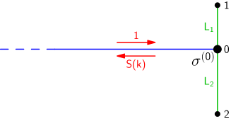
Figure 2: A simple model graph consisting of two edges (green) and one scattering lead attached to the central vertex 0 (blue). In numerical calculations we use $L_{1}=(1+\sqrt{5})/8\approx 0.4045$ and $L_{2}=1-L_{1}\approx 0.5955$.

4.2 The S-matrix.

Using Eq. (1.4) we can now derive an expression for $S(k)$. The indices $h,h^{\prime}$ from Eq. (1.4) can be omitted, since there is just a single scattering channel. Defining $\phi_{1,2}(k)=e^{2ikL_{1,2}}$ we obtain

$$S(k) =\frac{\phi_{1}\phi_{2}-\frac{\phi_{1}+\phi_{2}}{2}}{1-\frac{\phi_{1}+\phi_{2}}{2}}$$ (37)

$$=\sum_{t_{1},t_{2}=1}^{\infty}\frac{(t_{1}+t_{2})-(t_{1}-t_{2})^{2}}{2^{t_{1}+t_{2}}\,t_{1}t_{2}}\binom{t_{1}+t_{2}-2}{t_{1}-1}\,\phi_{1}^{t_{1}}\phi_{2}^{t_{2}}-\sum_{t=1}^{\infty}\frac{\phi_{1}^{t}+\phi_{2}^{t}}{2^{t}}$$ (38)

(see A for details). The first line of is a compact representation which is suitable for numerical calculations and clearly highlights the resonance structure of the scattering matrix. The second line is an expansion of $S(k)$ in terms of families of isometric trajectories starting and ending on the scattering lead. These families are labelled by pairs $\alpha=(t_{1},t_{2})$ counting the number of reflections from the the first and second outer vertex, respectively. Trajectories which are restricted to a single edge are accounted for by the second sum. In the notation of Eq. (21) the numbers q defining a family count the traversals of directed bonds. However, in our simple model, an edge is always traversed outward and inward successively, thus $q_{0\to 1}=q_{1\to 0}=t_{1}$ and $q_{0\to 2}=q_{2\to 0}=t_{2}$. We will refer to the integer value $t=t_{1}+t_{2}$ as the topological time of a path on the T-junction graph. As in Eq. (13) the oscillating phase factors $\phi_{1}^{t_{1}}\phi_{2}^{t_{2}}=\exp(ikl_{t_{1},t_{2}})$ in Eq. (38) depend on the total length of the trajectories within a family,

$$l_{t_{1},t_{2}}=2(t_{1}L_{1}+t_{2}L_{2})\,,$$ (39)

while the rational prefactors represent the sum of amplitudes from all trajectories within a family, as in Eq. (21).

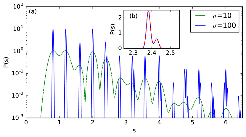
Figure 3: (a) The probability density $P(s)$ for a T-junction with $L_{1}=(1+\sqrt{5})/8\approx 0.4045$ and $L_{2}=1-L_{1}\approx 0.5955$. is shown for $\sigma=100$ (blue) and $\sigma=10$ (green broken line) on a logarithmic scale. (b) The inset enlarges a region where two peaks with almost degenerate trajectory lengths interfere ($\sigma=100$). The dashed red line in the inset is the interference pattern predicted by Eq. (19).

Fig. 3 shows the time delay density computed with Eqs. (16), (17), (37) by a Fourier transform of the scattering matrix $S(k)$. The two curves correspond to two different envelope widths $\sigma$. As predicted above in Eqs. (19), (20) a series of sharp peaks centered at the lengths of scattering trajectories develops as $\sigma$ grows. For example, the first two peaks at $s=2L_{1}\approx 0.81$ and $s=2L_{2}\approx 1.19$ each correspond to a single scattering trajectory which enters the graph, visits one of the outer vertices 1 or 2 and returns to the lead. However, to most of the peaks more than one trajectory contributes and their interference, expressed by the rational prefactors in Eq. (38), determines the height of the peak. For growing time $s$, an increasing fraction of peaks have a separation of the order of $\sim\sigma^{-1}$ or smaller and overlap. This is a limitation to Eq. (20) and the subsequent theory. An example at $3L_{1}\approx 2L_{2}\approx 2.4$ is magnified and compared to the prediction of Eq. (19) in the inset Fig. 3(b).

4.3 The topological delay time distribution.

Within the asymptotic approximation for broad envelope functions (short pulses), Eq. (20), we can evaluate the (cumulative) distribution of delay times (23) for the T-junction. According to Eqs. (21)-(23) the squared coefficients from Eq. (38) provide the weigth of a family and we obtain

$$C(s)= \sum_{t_{1},t_{2}=1}^{\infty}\left(\frac{(t_{1}+t_{2})-(t_{1}-t_{2})^{2}}{2^{t_{1}+t_{2}}\,t_{1}t_{2}}\binom{t_{1}+t_{2}-2}{t_{1}-1}\right)^{2}\,\Theta(s-l_{t_{1},t_{2}})$$

$$\qquad+\sum_{t=1}^{\infty}2^{-2t}\,[\Theta(s-l_{t,0})+\Theta(s-l_{0,t})]\,.$$ (40)

As in Eq. (25), this function can be bound from below and above by a variation of the edge lengths. Define $C(s,\ell)$ to denote the r.h.s of Eq. (40) with both edge lengths $L_{1}$, $L_{2}$ replaced by some value $\ell$ such that $l_{t_{1},t_{2}}$ is $2(t_{1}+t_{2})\ell$. Then the Heavyside functions in Eq. (40) are $\Theta(s-2t\ell)$ and select all terms with topological times $t=t_{1}+t_{2}$ up to $\lfloor{s/2\ell}\rfloor$ (the largest integer below $s/2\ell$). Thus, if $p_{t}$ denotes the sum of coefficients of all terms with some fixed topological time $t$, $C(s,\ell)$ is the cumulant sum

$$C(s,\ell)=\sum_{t=0}^{\lfloor{s/2\ell}\rfloor}p_{t}$$ (41)

Starting with the substitution $t_{2}=t-t_{1}$ we can evaluate $p_{t}$ as

$$p_{t} =2^{1-2t}+\sum_{t_{1}=1}^{t-1}\left(2^{-t}\frac{t-(t-2t_{1})^{2}}{t_{1}(t-t_{1})}\binom{t-2}{t_{1}-1}\right)^{2}$$ (42)

$$=\frac{3}{4}\frac{4^{2-t}}{t(t-1)}\binom{2t-4}{t-2}\qquad(t>1)$$ (43)

$$\approx\frac{3}{4}\frac{t^{-5/2}}{\sqrt{\pi}}\hskip 68.2866pt(t\to\infty)$$ (44)

while $p_{0}=0$ and $p_{1}=1/2$. Eq. (43) can be found with the help of standard computer algebra, and a formal proof can be based on the methods outlined in [21]. $p_{t}$ is a normalized discrete probability distribution (the distribution of topological time delays) and its cumulant sum is

$$c_{t} =\sum_{t^{\prime}=0}^{t}p_{t^{\prime}}$$ (45)

$$=1-\frac{2}{4^{t}t}\binom{2t-2}{t-1}$$ (46)

$$\approx 1-t^{-3/2}/\sqrt{4\pi}\qquad(t\to\infty)\,.$$ (47)

Now consider $C(s,L_{1})$ and $C(s,L_{2})$. Assuming without loss of generality $L_{1}<L_{2}$ we have $2(t_{1}+t_{2})L_{1}\leq l_{t_{1},t_{2}}\leq 2(t_{1}+t_{2})L_{2}$, i.e. in comparison with $C(s)$ the Heaviside steps occur in $C(s,L_{1})$ for smaller and in $C(s,L_{2})$ for larger values of $s$ while the coefficients remain unchanged. Hence

$$C(s,L_{2})\leq C(s)\leq C(s,L_{1})$$ (48)

Asymptotically for large delay $s\to\infty$ these bounds on $C(s)$ are explicitly given by substitution of $s/2L_{1,2}$ into Eq. (47),

$$1-\frac{(s/2L_{2})^{-3/2}}{\sqrt{4\pi}}\leq C(s)\leq 1-\frac{(s/2L_{1})^{-3/2}}{\sqrt{4\pi}}\qquad(s\to\infty)\,.$$ (49)

We conclude that the probability $1-C(s)$ to measure a delay larger than $s$ falls off as a power law with exponent $-3/2$ and that for $2L_{1}\lesssim 1\lesssim 2L_{2}$ a prefactor $1/\sqrt{4\pi}$ should be expected.

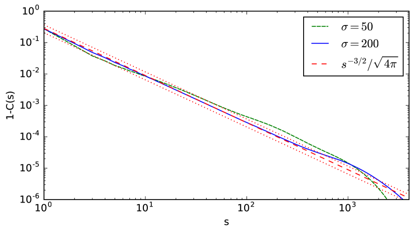
Figure 4: The long-time tail of the integrated delay-time distribution is shown on a double logarithmic scale for $\sigma=50$ (broken green line) and $\sigma=200$ (blue). The dashed red line is the theoretical result (52) based upon the distribution of narrow resonances. The upper and the lower dotted lines are the bounds (49) derived from the topological delay time distribution. For the calculations we used $k_{0}=1.000$ and a discrete Fourier transform of the S-matrix (37) on a grid with a spacing $\delta k\sim 10^{-4}$ which ensures convergence of the distribution in the displayed region $s\leq 4.000$.

4.4 The long-time delay distribution.

For $s\to\infty$ the factor $e^{-iks}$ in the Fourier integral of Eq. (16) has very fast oscillations which cancel out unless $S(k)$ is rapidly changing too. Therefore the asymptotic time delay for large $s$ is related to narrow resonances of the scattering matrix. On this basis we can develop an alternative approach to the delay time distribution, similar to [22, 23]. In B we show that $C(s)$ for large $s$ can be approximated by the sum

$$C(s) =1-4\pi\sum_{n}\omega^{2}(\kappa_{n})\gamma_{n}e^{-2\gamma_{n}s}\,,$$ (50)

where $\kappa_{n}-i\gamma_{n}$ are the poles of the scattering matrix (37) in the complex $k$-plane. For broad envelope functions $\omega(k)$ many resonances contribute and we can approximate Eq. (50) by an integral over the resonant wave number $\kappa$ and the resonance width $\gamma$,

$$C(s) =1-4\pi\int_{0}^{\infty}d\kappa\int_{0}^{\infty}d\gamma\,\rho(\kappa,\gamma)\,\omega^{2}(\kappa)\gamma\,e^{-2\gamma s}$$ (51)

$$=1-\frac{1}{\sqrt{4\pi}}\left(\frac{s}{L}\right)^{-3/2}\,,$$ (52)

where $L=L_{1}+L_{2}$ is the total length of the graph,

$$\rho(\kappa,\gamma)=\frac{1}{\pi^{2}}\sqrt{\frac{L^{3}}{2\gamma}}$$ (53)

is the average density of resonances in the complex plane and the normalization of $\omega(k)$ was used to integrate over $\kappa$ (see B for details). Clearly, Eq. (52) is compatible with Eq. (49) and even refines this prediction from the previous subsection. Moreover it becomes clear, that a condition for this result is that the envelope function covers many resonances with a relevant contribution in Eq. (50), i.e. with a width up to $\gamma(s)\sim s^{-1}$. Since $\rho(k,\gamma)\sim\gamma^{-1/2}$ the number of contributing resonances scales as $\sigma\sqrt{\gamma(s)}$ and we infer that Eq. (51) is valid up to a maximum time $s\sim\sigma^{2}$. Beyond that value $C(s)$ will have a non-universal behaviour dictated by the resonances with the smallest widths which are covered by the envelope function.

Fig. 4 illustrates the results from the previous and the present subsections. In order to highlight the power-law tail of the delay time distribution we show the quantity $1-C(s)=\int_{s}^{\infty}ds^{\prime}P(s^{\prime})$, i.e. the probability to measure a delay exceeding $s$. We compare numerical results for $\sigma=50$ and $\sigma=200$ to the bounds derived from the topological delay time in Section 4.3 and to Eq. (52) above. For $\sigma=200$ there is a very good agreement up to $s\sim 300$. Beyond $s=3.000$ $P(s)$ falls off very fast because the region covered by the envelope function contains no resonances which are narrow enough to contribute. For smaller $\sigma$ the deviations set in earlier and are generally larger, as expected.

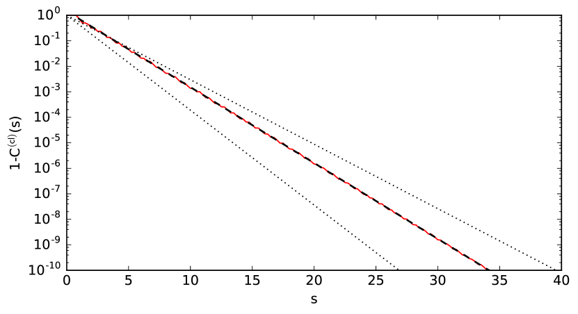
Figure 5: The classical delay-time distribution is shown on a logarithmic scale with a red line. The dashed line is the theoretical result (59) for $\xi\approx 0.6846$ (the numerical root of Eq. (57)). The dotted lines are the upper and the lower bounds on $C^{(cl)}(s)$ derived from the topological delay distribution.

4.5 The clasical delay distribution.

According to Eq. (29), for the clasical delay distribution we have to sum over all paths leading from the scattering channel into the graph and back to the channel. For the T-junction these paths consist of $t_{1}$ excursions from the central vertex 0 to vertex 1 and $t_{2}$ excursions to vertex 2, in arbitrary order. The total length of such a path was given in Eq. (39). The product of matrix elements of $\tilde{M}$ along the path is $4^{-(t-1)}$, corresponding to $t-1$ inner crossings of vertex 0 (see C for details). Again $t=t_{1}+t_{2}$ denotes the topological time. Together with the probabilities $|\tau_{h,d_{0}}|^{2}=|\tau_{h,d_{n}}|^{2}=1/2$ for entering and leaving the interior graph from/to the scattering channel the weight of each path is $4^{-t}$. The number of paths with given $t_{1}$ and $t_{2}$ is easily counted and thus from Eq. (29) we find for the T-junction

$$C^{(cl)}(s)=\sum_{t_{1},t_{2}}^{\infty}4^{-(t_{1}+t_{2})}\binom{t_{1}+t_{2}}{t_{1}}\Theta(s-l_{t_{1},t_{2}})\,.$$ (54)

Similar to Eq. (48) we can estimate this quantity by substitution of a common value $\ell$ for the edge lengths. As there are $2^{t}$ paths with topological time $t$ we have

$$C^{(cl)}(s,\ell) =\sum_{t=1}^{\infty}2^{-t}\Theta(s-2t\ell)$$ (55)

$$=1-2^{-\lfloor s/2\ell\rfloor}\,.$$ (56)

With $\ell=L_{1}$ ($\ell=L_{2}$) this expression is an upper (lower) bound for $C^{(cl)}(s)$. However, a much more precise estimate can be obtained from Eq. (35). For the T-junction we find

$$\det(1-\tilde{M}(-\xi))=1-\frac{1}{4}e^{2L_{1}\xi}-\frac{1}{4}e^{2L_{2}\xi}=0$$ (57)

and can solve for $\xi$. Then, integrating Eq. (35) with respect to $s$ we have

$$C^{(cl)}(s) =1-\int_{s}^{\infty}ds^{\prime}\,P^{(cl)}(s^{\prime})$$ (58)

$$\approx 1-\frac{A(\xi)}{\xi}e^{-\xi s}\qquad(s\to\infty)$$ (59)

where

$$A(\xi) =\frac{2}{L_{1}\,e^{2\xi L_{1}}+L_{2}\,e^{2\xi L_{2}}}$$ (60)

dentotes the sum in Eq. (35) for a T-junction. See C for more details on the derivation of these results.

Note that Eq. (57) requires a numerical solution in general. A full analytical soltion can be given, e.g., for a T-junction with two edges of equal length, $L_{1}=L_{2}=1/2$. Expanding around this trivial case to leading order in the difference of the edge lengths $\delta L=L_{2}-L_{1}$ for fixed $L_{1}+L_{2}=1$ one finds $\xi\approx\ln 2\cdot(1-\frac{\ln 2}{2}[\delta L]^{2})$ and $A(\xi)=1-\ln 2\cdot[\delta L]^{2}$.

Fig. 5 illustrates our results for the classical delay distribution and shows a very accurate agreement between Eq. (60) and numerical data generated from Eq. (54).

5 Conclusions

In the preceding sections we have provided a theory for the computation of the delay time distribution in scattering from quantum (wave-guide) networks. A main result was the reduction of the distribution to a purely combinatorial expression, the topological delay time distribution of Eq. (24). It provides bounds for the actual distribution which do not depend on the precise lengths of the edges of the network as long as they are not rationally related.

In the last chapter we have given a complete solution for a simple graph, which reveals remarkable features. The coherent delay time distribution decays as a power-law while the classical distribution shows the expected exponential decay, emphasizing the importance of interferences effects when the scattering region supports a complex internal dynamics. From another perspective the algebraic decay is related to a particular distribution of the widths of long-lived scattering resonances which in this simple model was analytically accessible.

The methods developed in the present paper and tested in the toy model of Section 4 can now be applied to quantum graphs with a physically more interesting and challenging structure. To name an example, scattering from random non compact graphs is now under study, showing the effects of Anderson localization in the time domain. The results will be reported shortly.

6 Acknowledgements

Professor Steve Anlage is acknowledged for directing us to the subject, by sharing his preliminary experimental results. US acknowledges support from the Humboldt foundation.

Appendix A

Here we evaluate the scattering matrix for the T-junction-model of Section 4 starting from Eq. (1.4) and Eq. (36). There is only a single scattering channel $h=h^{\prime}=0$. The amplitude for direct reflection

$$\rho_{0}=0$$

is given by the first element of the matrix $\sigma^{(0)}$ in Eq. (36).

The transition amplitudes $\tau_{d0}$ from the scattering channel into the graph are non-zero only if the directed bond $d$ points outward from the central vertex ($0\to 1$, $0\to 2$). Vice versa the transition amplitudes $\tau_{0d}$ are non-zero for inward pointing bonds ($1\to 0$, $2\to 0$). According to Eq. (36) each non-zero transition amplitude is $\pm\sqrt{2}/2$, and their product has negative/positive sign if the first and the last edge traversed inside the graph are equal/distinct.

The matrix $W$ has dimension 4 and is explicitly given by

$$W(k)=\begin{pmatrix}0&0&\frac{1}{2}e^{ikL_{1}}&\frac{1}{2}e^{ikL_{1}}\\[2.84526pt] 0&0&\frac{1}{2}e^{ikL_{2}}&\frac{1}{2}e^{ikL_{2}}\\[2.84526pt] e^{ikL_{1}}&0&0&0\\[2.84526pt] 0&e^{ikL_{2}}&0&0\end{pmatrix}$$ (61)

where we have ordered the four directed bonds of the graph such, that the first two entries correspond to bonds from the central vertex outward and the last two entries to bonds directed inward. For compact notation we define

$$\phi_{1,2}(k)=e^{2ikL_{1,2}}$$ (62)

and find $\det(I-W)=1-(\phi_{1}+\phi_{2})/2$. Now it is possible to calculate $(I-W)^{-1}$ using the adjugate of $I-W$. In fact, it suffices to calculate the lower left 2$\times$2 block of the adjugate (outward to inward)

$$\frac{1}{2}\begin{pmatrix}e^{ikL_{1}}(2-e^{2ikL_{2}})&e^{ik(2L_{1}+L_{2})}\\ e^{ik(L_{1}+2L_{2})}&e^{ikL_{2}}(2-e^{2ikL_{1}})\\ \end{pmatrix}$$

because only for this combination the product $\tau_{h,d}\tau_{d^{\prime},h}$ in Eq. (1.4) is non-zero and equal to $\pm 1/2$ (minus on the diagonal of the block). According to Eq. (1.4), the first and second column are also multiplied by $e^{ikL_{1}}$ and $e^{ikL_{2}}$, respectively. Summation of all four matrix elements finally yields Eq. (37). In order to arrive at Eq. (38) we can expand the denominator as a geometric series and regroup all terms according to the powers in $\phi_{1}$ and $\phi_{2}$.

As an alternative, Eq. (38) can also be obtained directly from a summation of all paths on the graph as in Eq. (13). A path consists of several excursions from the central vertex 0 to either vertex 1 or vertex 2 and back to zero. Each such excursion contributes a phase $\phi_{1}$ or $\phi_{2}$, respectively. Moreover, there is a transion amplitude $1/2$ for every internal transition across vertex 0 and an amplitude $\pm 1/\sqrt{2}$ for a transition from the scattering channel into the graph and back. Therefore each path with $t_{1}+t_{2}$ excursions has an amplitude $\pm 2^{-(t_{1}+t_{2})}$. Paths of the form 1…2 or 2…1 have a positive sign and are counted by choosing the positions of the $n_{1}-1$ remaining excursions to vertex 1 from the $t_{1}+t_{2}-2$ available inner time steps. Paths of the form 1…1 or 2…2 have negative sign and are counted in an analogous way. We obtain

$$S=\sum_{t_{1},t_{2}=0}^{\infty}\left[2\binom{t_{1}+t_{2}-2}{t_{1}-1}-\binom{t_{1}+t_{2}-2}{t_{1}-2}-\binom{t_{1}+t_{2}-2}{t_{2}-2}\right]\,\frac{\phi_{1}^{t_{1}}\phi_{2}^{t_{2}}}{2^{t_{1}+t_{2}}}\,.$$ (63)

After applying binomial recursion (Pascal’s triangle) to the second and the third binomial, the first binomial can be factored out and the equivalence to Eq. (38) is easily established.

Appendix B

As obvious from Eq. (37), the scattering matrix has a singularity if $\phi_{1}(k)+\phi_{2}(k)=2$. For real $k>0$ this equation has no solution since it would imply $\phi_{1}(k)=\phi_{2}(k)=1$, i.e. $kL_{1,2}=2m_{1,2}\pi$ and $L_{1}/L_{2}=m_{1}/m_{2}$ for integer $m_{1}$ and $m_{2}$. This is excluded by the incommensurability of the bond lengths. However it is possible that the two phases pass through a multiple of $2\pi$,

$$e^{2ik_{1}L_{1}}=e^{2ik_{2}L_{2}}=1\,.$$ (64)

at two different wave numbers $k_{1}$ and $k_{2}$ which have a very small spacing

$$\delta k=|k_{1}-k_{2}|\,.$$ (65)

We define

$$L =L_{1}+L_{2}$$ (66)

$$\lambda =\frac{L_{1}L_{2}}{L}$$ (67)

$$\gamma =\frac{\lambda^{2}}{L}\delta k^{2}$$ (68)

and a weighted average of $k_{1}$ and $k_{2}$,

$${\kappa} =\frac{k_{1}L_{1}+k_{2}L_{2}}{L}$$ (69)

It is easy to verify that $S(k_{1})=S(k_{2})=-1$ and $S(\kappa)=+1$, i.e. the phase of the S-matrix completes a full cycle in the small interval between $k_{1}$ and $k_{2}$. In the immediate vicinity of $\kappa$ the functional form of the phase is universal when $k-\kappa\sim\delta k^{2}$. Namely, using Eq. (64) we have

$$\phi_{1}(k) =e^{2ikL_{1}}\approx 1+2i\lambda\delta k+2iL_{1}\delta k-2\lambda^{2}\delta k^{2}$$ (70)

$$\phi_{2}(k) =e^{2ikL_{2}}\approx 1-2i\lambda\delta k+2iL_{2}\delta k-2\lambda^{2}\delta k^{2}$$ (71)

$$S(k) \approx-\frac{k-(\kappa+i\gamma)}{k-(\kappa-i\gamma)}$$ (72)

$$=e^{2i\arctan([k-\kappa]/\gamma)}\,.$$ (73)

Note that due to cancellations Eq. (72) is valid to leading order in $\delta k$ only, although $\phi_{1,2}(k)$ were expanded to second order. From this result it is obvious that the scattering matrix has a pole close to the real axis at $\kappa-i\gamma$. For a resonance of width $\gamma$ the maximal derivative of the phase in Eq. (73) is $2/\gamma$. Up to this value of $s$ the Fourier integral in Eq. (16) has a point of stationary phase and thus a relevant contribution to $P(s)$ results. In the vicinity of $\kappa$ we can approximate the envelope function by the constant $\omega(\kappa)$. The resulting contribution is then found from the residue $2i\gamma\,e^{-i\kappa s-\gamma s}$ of the remaining integrand at the pole. Summation over all resonances gives

$$P(s) =\frac{1}{2\pi}\left|4\pi\sum_{n}\gamma_{n}\omega(\kappa_{n})\,e^{-i\kappa_{n}s-\gamma_{n}s}\right|^{2}\,.$$ (74)

In this expression the contributions from different resonances $n$ to $P(s)$ will interfere. However, in $C(s)$ the integration with respect to $s$ will destroy these interferences. To see this, expand $|\dots|^{2}$ as a double sum over $n,n^{\prime}$. Then nondiagonal terms have oscillating phase factors $e^{i(\kappa_{n}-\kappa_{n^{\prime}})s}$ and are suppressed in comparison to the diagonal terms $n=n^{\prime}$. We are left with

$$C(s) =1-8\pi\int_{s}^{\infty}ds^{\prime}\sum_{n}\omega^{2}(\kappa_{n})\gamma_{n}^{2}e^{-2\gamma_{n}s}$$ (75)

which finally yields Eq. (50). Further the sum over resonances can be replaced by the integral Eq. (51) if the envelope function is broad and a large number of resonances contribute. In this way the delay distribution for long times is related to the density of narrow resonances in the complex plane. In order to estimate this density $\rho(\kappa,\gamma)$ we first note that points $k_{1}$ with $e^{2ik_{1}L_{1}}$ have a density $L_{1}/\pi$. At these points the second phase $\varphi_{2}(k_{1})=2k_{1}L_{2}$ can be treated as a random number with uniform distribution between $\pm\pi$. If $|\varphi_{2}|$ is small, a small change $\delta k=-\varphi_{2}/2L_{2}$ is sufficient to bring it to zero. Thus a spacing between 0 and $\delta k$ results with probability $2\delta kL_{2}/\pi$. Then $2L_{1}L_{2}\delta k/\pi^{2}=\sqrt{2\gamma L^{3}}/\pi^{2}$ is the probability to find a resonance with width smaller than $\gamma$ per unit $k$-interval. This is equivalent to Eq. (53).

Appendix C

For the T-junction, the matrix elements of $\tilde{M}$ in Eq. (29) are the absolute squares of the elements of $\tilde{W}$ in Eq. (61),

$$\tilde{M}=\begin{pmatrix}0&0&\frac{1}{4}&\frac{1}{4}\\[2.84526pt] 0&0&\frac{1}{4}&\frac{1}{4}\\ 1&0&0&0\\ 0&1&0&0\end{pmatrix}\,.$$ (76)

The upper right block contains the probabilities to scatter from a bond directed inward ($1\to 0$ or $2\to 0$) into an outward bond ($0\to 1$ or $0\to 2$). The lower left block represents the probabilities for the opposite process. This block is a 2$\times$2 unit matrix because along a path on the graph the bond $0\to 1$ is always followed by $1\to 0$ and the same holds for $0\to 2$, $2\to 0$. Thus each path contains an even number $2t$ of directed bonds, where the topological time $t=t_{1}+t_{2}$ counts the number of excursions to vertex $1$ or vertex $2$. A path with topological time $t$ pics up $t$ matrix elements 1 from the lower left and $t-1$ elements $1/4$ from the upper right block, i.e. it has a weight $4^{1-t}$ (excluding the probabilities to enter (leave) the interior graph at the start (end) of the path.

For $\tilde{M}(z)$ in Eq. (32) we find from Eq. (76) and with the substitution $x_{1,2}(z)=e^{-zL_{1,2}}$

$$\tilde{M}(z)=\frac{1}{4}\begin{pmatrix}0&0&x_{1}&x_{1}\\[2.84526pt] 0&0&x_{2}&x_{2}\\ 4x_{1}&0&0&0\\ 0&4x_{2}&0&0\end{pmatrix}\,.$$ (77)

and a straightforward calculation yields

$$\det(1-\tilde{M}(z)) =1-\frac{x_{1}^{2}}{4}-\frac{x_{2}^{2}}{4}$$ (78)

$$=1-\frac{1}{4}e^{-2L_{1}z}-\frac{1}{4}e^{-2L_{2}z}$$ (79)

$$\frac{d}{dz}\det(1-\tilde{M}(z)) =\frac{L_{1}}{2}e^{-2L_{1}z}+\frac{L_{2}}{2}e^{-2L_{2}z}$$ (80)

To complete the information required in Eq. (35) we need the adjugate of $I-\tilde{M}(z)$. As in the calculation of $S$ in A it suffices to calculate the lower left block (outward to inward)

$$\frac{1}{4}\begin{pmatrix}4x_{1}-x_{1}x_{2}^{2}&x_{1}^{2}x_{2}\\ x_{1}x_{2}^{2}&4x_{2}-x_{1}^{2}x_{2}\end{pmatrix}\,.$$

Only for these matrix elements one the factor $|\tau_{d,0}\tau_{d^{\prime},0}|^{2}$ is non-zero and has the value 1/4. Finally the sum over $d,d^{\prime}$ in Eq. (35) yields $(x_{1}(z)^{2}+x_{2}(z)^{2})/4=1-\det(I-\tilde{M}(z))$. In particular, at a zero of the determinat this is just 1.

References

References

- [1] Smilansky U 2017 Journal of Physics A: Mathematical and Theoretical 50 215301
- [2] Eckle P et al. 2008 Science 1525–1529
- [3] Landsman A S et al. 2014 Optica 1 343–349
- [4] Hassan M T et al. 2016 Nature 530 66–70
- [5] Max Planck Institute of Quantum Optics and Ludwig Maximilians University Munich 2015 Attosecond physics: Film in 4-d with ultrashort electron pulses phys.org/news/2015-10-attosecond-physics-d-ultrashort-electron.html
- [6] Kottos T and Smilansky U 1997 Phys. Rev. Lett. 79 4794–4797
- [7] Kottos T and Smilansky U 1999 Ann. Phys. 274 76–124
- [8] Gnutzmann S and Smilansky U 2006 Advances in Physics 55 527–625
- [9] Berkolaiko G and Kuchment P 2013 Introduction to Quantum Graphs (American Mathematical Society)
- [10] Band R, Berkolaiko G and Smilansky U 2012 Annales Henri Poincaré 13 145–184
- [11] Anlage S 2016 (private communication)
- [12] Sirko L 2017 (private communication)
- [13] Kostrykin V and Schrader R 1999 J. Phys. A 32 595–630
- [14] Kottos T and Smilansky U 2003 J. Phys. A 36 3501–3524
- [15] Schanz H and Smilansky U 2000 Phys. Rev. Lett. 84 1427–1430
- [16] Schanz H and Smilansky U 2000 Phil. Mag. B 80 1999–2021
- [17] Gavish U and Smilansky U 2007 Journal of Physics A: Mathematical and Theoretical 40 10009
- [18] Kiro A, Smilansky Y and Smilansky U 2016 e-print ArXiv.org/abs/1608.00150
- [19] Parry W 1983 Israel Journal of Mathematics 45 41–52
- [20] Kostrykin V and Schrader R 2000 Fortschritte der Physik 48 703–716
- [21] Petkovšek M, Wilf H S and Zeilberger D 1996 A=B (Wellesley, Massachusetts: AK Peters)
- [22] Dittes F M, Harney H L and Müller A 1992 Phys. Rev. A 45 701–705
- [23] Hart J A, Antonsen T M and Ott E 2009 Phys. Rev. E 79 016208