Interaction between two point-like charges in nonlinear electrostatics

Abstract

We consider two point-like charges in electrostatic interaction between them within the framework of a nonlinear model, associated with QED, that provides finiteness of their field energy. We find the common field of the two charges in a dipole-like approximation, where the separation between them $R$ is much smaller than the observation distance $r:$ with the linear accuracy with respect to the ratio $R/r$, and in the opposite approximation, where $R\gg r,$ up to the the term quadratic in the ratio $r/R$. The consideration fulfilled proposes the law $a+bR^{1/3}$ for the energy, when the charges are close to one another, $R\rightarrow 0$. This leads to the singularity of the force between them to be $R^{-2/3}$, which is weaker than Coulomb law $R^{-2}$.

I Introduction

Recently a class of nonlinear electrodynamic models was studied CosGitSha2013a wherein the electrostatic field of a point charge is, as usual, infinite in the point, where the charge is located, but this singularity is weaker than that of the Coulomb field, so that the space integral for the energy stored in the field converges (and also the scalar potential is finite in the position of the charge AdoGitShaShi2016 ). This class unites Lagrangians AdoGitShaShi2016 - Ependiev that grow with the field invariant $\mathfrak{F=}\left(B^{2}-E^{2}\right)/2$ faster than $(-\mathfrak{F)}^{w},w>$ $3/2$ (see Ref. AdoGitShaShi2016 also for a subtler estimate of the boundary of the necessary growth). Thus, the simple quadratic effective Lagrangian first considered in a different aspect in Kruglov2008 is also included into the class under consideration.

The infiniteness of the field near the charge distinguishes the class under consideration from many other models (see the papers Kruglov and references therein) with finite self-energy of the point charge, allied to their famous prototype, the Born-Infeld model Born-Infeld , where the finiteness of the field is achieved at the cost of square-root nonanalyticity of the Lagrangian that supplies an infinity to the Maxwell equation. The most popular application Kruglov , Hendi of these models is to combine them with the General Relativity in order to study their effect on the initial singularity and on the evolution of the Universe. In contrast to the Born-Infeld model, the models from the class of Ref. CosGitSha2013a refer to nonsingular Lagrangians that follow for instance from the Euler-Heisenberg (E-H) effective Lagrangian Heisenberg of QED truncated at any finite power of its Taylor expansion in the field. This allows us to identify the self-coupling constant of the electromagnetic field with a definite combination of the electron mass and charge and to propose that such models may be used to extend QED to the extreme distances smaller than those for which QED may be thought of as a perfectly adequate theory.

More advanced approaches based on the Euler-Heisenberg Lagrangian that do not depend upon any assumption of smallness of its field argument (the background field) and do not hence appeal to expansion of the Lagrangian in powers of the background fields received attention, as well, under the restriction, however, that not-too-fast-varying in space and time fields are studied as solutions of the nonlinear Maxwell equations. Among the nonlinear effects studied, there are the linear and quadratic electric and magnetic responses of the vacuum with a strong constant field in it to an applied electric field AdoGitSha2016 , with the emphasis on the magneto-electric effect GitSha2012 ; AdoGitSha2013 and magnetic monopole formation AdoGitSha2015 . Also self-interaction of electric and magnetic dipoles was considered with the indication that the electric and magnetic moments of elementary particles are subjected to a certain electromagnetic renormalization CosGitSha2013 after being calculated following a strong-interaction theory, say, QCD or lattice simulations. Interaction of two laser beams against the background of a slow electromagnetic wave was studied along these lines, too King . The finiteness of the field energy allows one to develop a soliton view on a moving point charge movingPreprint , Shishmarev .

In the present paper we are extending the consideration to cover the electrostatic problem of a system of two point charges that interact following nonlinear Maxwell equations stemming from the Lagrangian quadratic in the the field invariant $\mathfrak{F}$. Their common field is not, of course, just a linear combination of the individual fields of the two charges. The nonlinear problem is outlined in the next Section II, where we present the nonlinear Maxwell equations and give them the form in Subsection II.2 apt for finding the approximate solutions of Section III. Once the field energy is finite it is possible in principle to define the attraction or repulsion force between charges as the derivative of the field energy with respect to the distance $\mathbf{R}$ between them. Contrary to the standard linear electrodynamics, this is evidently not the same as the product of one charge by the field strength produced by the other! This rule holds true only if one of the charges is much smaller in value than the other.

In Section III we develop the procedure of finding the solution to the static two-body problem in two opposite approximations determined by the ratio of the distance $R,$ to the coordinate of the observation point $r$. Where this ratio is small, $R/r\ll 1$, we find in Subsection III.1 the leading expression for the common field, which makes the nonlinear correction to electric dipole, and the corresponding potential. In Subsection (III.2)) the opposite case $r/R\ll 1$ is considered, first, also in the leading approximation (Subsubsection III.2.1). The simplifying circumstance that makes these approximations easy to handle is that it so happens that one needs, as a matter of fact, to solve only the second (following the classification of Ref. Landau ) Maxwell equation, the one following from the least action principle, while the first one, the Bianchi identity, $\left[\mathbf{\nabla\times E}\right]=0,$ is trivially satisfied. The situation becomes far more complicated in the next-to-leading approximation $\left({r}/{R}\right)^{2}$ developed in Subsubsection III.2.2. In developing the above approximations no assumption was made on whether the nonlinear scale determined by the self-coupling of the electromagnetic field is large or small as compared to $r$ or $R.$ Their use in the expression for the energy of the two charges as a function of the separation $R$ in the limit $R\rightarrow 0,$ i.e. when the charges are so close to one another that $R$ is much less than the nonlinearity scale, allows to make a preliminary estimation confirmed by another approach to be reported in a separate publication that for small separation, the energy of the system of two point charges can be presented as $a+bR^{1/3},$ where $a$ and $b$ are finite constants depending only on the two charges (in QED they include the electron mass and charge). Hence the force between two point-like charges turns to infinity following the law $R^{-2/3}.$ This formula replaces, in the given nonlinear model, the Coulomb law $R^{-2}$ for the force between two point charges.

II Nonlinear Maxwell equations

II.1 Nonlinear Maxwell equations as they originate from QED

It is known that QED is a nonlinear theory due to virtual electron-positron pair creation by a photon. The nonlinear Maxwell equation of QED for the electromagnetic field tensor $F_{\nu\mu}\left(x\right)=\partial^{\mu}A^{\nu}(x)-\partial^{\nu}A^{\mu}(x)$ $(\tilde{F}_{\tau\mu}\left(x\right)$ designates its dual tensor $\tilde{F}^{\mu\nu}=\left(1/2\right)\varepsilon^{\mu\nu\rho\sigma}F_{\rho\sigma}$ ) produced by the classical source  $J_{\mu}\left(x\right)$ may be written as, see e.g. AdoGitSha2016 .

$$\partial^{\nu}F_{\nu\mu}\left(x\right)-\partial^{\tau}\left[\frac{\delta\mathcal{L}\left(\mathfrak{F,G}\right)}{\delta\mathfrak{F}\left(x\right)}F_{\tau\mu}\left(x\right)+\frac{\delta\mathcal{L}\left(\mathfrak{F,G}\right)}{\delta\mathfrak{G}\left(x\right)}\tilde{F}_{\tau\mu}\left(x\right)\right]=J_{\mu}\left(x\right)\,$$ (1)

Here $\mathcal{L}\left(\mathfrak{F,G}\right)$ is the effective Lagrangian (a function of the two field invariants $\mathfrak{F}=(1/4)F^{\mu\nu}F_{\mu\nu}$ and $\mathfrak{G}=\left(1/4\right)\tilde{F}^{\mu\nu}F_{\mu\nu}),$ of which the generating functional of one-particle-irreducible vertex functions, called effective action weinberg , is obtained by the space-time integration as $\textstyle\Gamma\left[A\right]=\int\mathcal{L}\left(x\right)d^{4}x.$ Eq. (1) is the realization of the least action principle

$$\frac{\delta S\left[A\right]}{\delta A^{\mu}\left(x\right)}=\partial^{\nu}F_{\nu\mu}\left(x\right)+\frac{\delta\Gamma\left[A\right]}{\delta A^{\mu}\left(x\right)}=J_{\mu}(x),$$

where the full action $S\left[A\right]=S_{\mathrm{Maxw}}\left[A\right]+\Gamma\left[A\right]$ includes the standard classical, Maxwellian, electromagnetic action $S_{\mathrm{Maxw}}\left[A\right]=-\int\mathfrak{F}\left(x\right)d^{4}x$ with its Lagrangian known as $L_{\text{Maxw}}=-\mathfrak{F}=(1/2)\left(E^{2}-B^{2}\right)$ in terms of the electric and magnetic fields, $\mathbf{E}$ and $\mathbf{B}.$

Eq. (1) is reliable only as long as its solutions vary but slowly in the space-time variable $x_{\mu},$ because we do not include the space and time derivatives of $\mathfrak{F}$ and$\mathfrak{\ G}$ as possible arguments of the functional $\Gamma\left[A\right]$ treated approximately as local. This infrared, or local approximation shows itself as a rather productive tool AdoGitSha2016 – King . The calculation of one electron-positron loop with the electron propagator taken as solution to the Dirac equation in an arbitrary combination of constant electric and magnetic fields of any magnitude supplies us with a useful example of $\Gamma\left[A\right]$ known as the E-H effective action Heisenberg . It is valid to the lowest order in the fine-structure constant $\alpha$, but with no restriction imposed on the the background field, except that it has no nonzero space-time derivatives. Two-loop expression of this local functional is also available Ritus .

The dynamical Eq. (1), which makes the "second pair" of Maxwell equations, may be completed by postulating also their "first pair"

$$\partial_{\nu}\widetilde{F}^{\nu\mu}\left(x\right)=0,$$ (2)

whose fulfillment allows using the 4-vector potential $A^{\nu}(x)$ for representation of the fields: $F_{\nu\mu}\left(x\right)=\partial^{\mu}A^{\nu}(x)-\partial^{\nu}A^{\mu}(x).$ This representation is important for formulating the least action principle and quantization of the electromagnetic field. From it, Eq. (2) follows identically, unless the potential has the angular singularity like the Dirac string peculiar to magnetic monopole. In the present paper we keep to Eq. (2), although its local denial is not meaningless, as discussed in Refs. AdoGitSha2015 , where a magnetic charge is produced in nonlinear electrodynamics.

We are going now to separate the electrostatic case. This may be possible if the reference frame exists where all the charges are at rest, $J_{0}(x)=J_{0}(\mathbf{r})$ (We denote $\mathbf{r=x}$). Then in this "rest frame" the spacial component of the current disappears, $\mathbf{J}\left(x\right)=0,$ and the purely electric time-independent configuration $F_{ij}\left(\mathbf{r}\right)=0$ would not contradict equation (1). With the magnetic field equal to zero, the invariant $\mathfrak{G=}$ $\left(\mathbf{E}\cdot\mathbf{B}\right)$ disappears, too. In a theory even under the space reflection, to which class QED belongs, also we have $\textstyle\left.\frac{\partial\mathcal{L}\left(\mathfrak{F,G}\right)}{\partial\mathfrak{G}\left(x\right)}\right|_{\mathfrak{G}=0}=0$, since the Lagrangian should be an even function of the pseudoscalar $\mathfrak{G}$. Then we are left with the equation for a static electric field $E_{i}=F_{i0}\left(\mathbf{x}\right)$

$$\partial_{i}F_{i0}\left(\mathbf{r}\right)-\partial_{i}\frac{\delta\mathcal{L}\left(\mathfrak{F,}0\right)}{\delta\mathfrak{F}\left(\mathbf{r}\right)}F_{i0}(\mathbf{r})=J_{0}\left(\mathbf{r}\right).\,$$ (3)

II.2 Generalities of solutions to nonlinear Maxwell equations

Equation (3) is seen to be the equation of motion stemming directly from the Lagrangian

$$L=-\mathfrak{F+}\mathcal{L}\left(\mathfrak{F,}0\right)$$ (4)

with the constant external charge $J_{0}\left(\mathbf{r}\right)$ and the zero argument set for the second field invariant $\mathfrak{G}.$ In the rest of the paper we shall be basing on this Lagrangian in understanding that it may originate from QED as described above or, alternatively, be given ad hoc to define a certain model. In the latter case, if treated seriously as applied to short distances near a point charge where the field cannot be considered as slowly varying, in other words, beyond the applicability of the infrared approximation of QED outlined above, the Lagrangian (4) may be referred to as defining an extension of QED to short distances once $\mathcal{L}\left(\mathfrak{F,}0\right)$ is the E-H Lagrangian (or else its multi-loop specification) restricted to $\mathfrak{G}=0$.

It was shown in CosGitSha2013a that the important property of finiteness of the field energy of the point charge is guarantied if $\mathcal{L}\left(\mathfrak{F,}0\right)$ in (4) is a polynomial of any power, obtained, for instance, by truncating the Taylor expansion of the H-E Lagrangian at any integer power of $\mathfrak{F}$. On the other hand, it was indicated in movingPreprint that a weaker condition is sufficient: if $\mathcal{L}\left(\mathfrak{F,}0\right)\mathfrak{\ }$grows with $-\mathfrak{F}$ as $\left(-\mathfrak{F}\right)^{w}$, the field energy is finite provided that $w>3/2$. The derivation of this condition is given in AdoGitShaShi2016 and in Ependiev . As a matter of fact a more subtle condition suffices: $\mathcal{L}\left(\mathfrak{F}\right)\sim\left(-\mathfrak{F}\right)^{\frac{3}{2}}\ln^{u}\left(-\mathfrak{F}\right),$  $u>2.$

In the present paper we confine ourselves to the simplest example of the nonlinearity generated by keeping only quadratic terms in the Taylor expansion of the E-H Lagrangian in powers of the field invariant $\mathfrak{F}$

$$\mathcal{L}\left(\mathfrak{F((}x)\mathfrak{,}0\right)=\frac{1}{2}\left.\frac{d^{2}\mathcal{L}\left(\mathfrak{F,}0\right)}{d^{2}\mathfrak{F}}\right|_{\mathfrak{F}=0}\mathfrak{F}^{2}\mathfrak{(}x),$$

where the constant and linear terms are not kept, because their inclusion would contradict the correspondance principle that does not admit changing the Maxwell Lagrangian $L_{\text{Max}}=-\mathfrak{F}$ for small fields. The correspondence principle is laid into the calculation of the E-H Lagrangian via the renormalization procedure.

Finally, we shall be dealing with the model Lagrangian quartic in the field strength

$$L=-\mathfrak{F(}x)\mathfrak{+}\frac{1}{2}\gamma\mathfrak{F}^{2}\mathfrak{(}x)$$ (5)

with $\gamma$ being a certain self-coupling coefficient with the dimensionality of the fourth power of the length, which may be taken as

$$\gamma=\left.\frac{d^{2}\mathcal{L}\left(\mathfrak{F,}0\right)}{d^{2}\mathfrak{F}}\right|_{\mathfrak{F}=0}=\frac{e^{4}}{45\pi^{2}m^{4}},$$ (6)

where $e$ and $m$ are the charge and mass of the electron, if $\mathcal{L}$ is chosen to be the E-H one-loop Lagrangian. We do not refer to this choice henceforward. Generalization to general Lagrangians can be also done in a straightforward way.

The second (3) and the first (2) Maxwell equations for the electric field $\mathbf{E}$ with Lagrangian (5) are

$$\mathbf{\nabla}\cdot\left[\left(1+\frac{\gamma}{2}E^{2}(\mathbf{r})\right)\mathbf{E}(\mathbf{r})\right]=j_{0}(\mathbf{r}),$$ (7)

$$\mathbf{\nabla}\times\mathbf{E}(\mathbf{r})=0.$$ (8)

Denoting the solution of the linear Maxwell equations as $\mathbf{E}^{lin}(\mathbf{r})$

$$\nabla\cdot\mathbf{E}^{lin}(\mathbf{r})=j_{0}(\mathbf{r}),\quad\mathbf{\nabla}\times\mathbf{E}^{lin}(\mathbf{r})=0,$$

we write the solution of (7), in the following way AdoGitSha2016 – CosGitSha2013

$$\left(1+\frac{\gamma}{2}E^{2}(\mathbf{r})\right)\mathbf{E}(\mathbf{r})=\mathbf{E}^{lin}(\mathbf{r})+[\mathbf{\nabla}\times\mathbf{\Omega}(\mathbf{r})],$$ (9)

because $\nabla\cdot$ $[\mathbf{\nabla}\times\mathbf{\Omega}(\mathbf{r})]=0.$

The second Maxwell equation (9) may be conveniently written in the form to be exploited later

$$\mathbf{E}(\mathbf{r})=\mathbf{N}(\mathbf{r})\xi\left(\gamma N^{2}(\mathbf{r})\right),\quad\mathbf{N}(\mathbf{r})=\mathbf{E}^{lin}(\mathbf{r})+\nabla\times\mathbf{\Omega}(\mathbf{r}),$$ (10)

where the function $\xi(x)$ is defined as the real solution to the cubic equation

$$\left(1+\frac{x}{2}\xi^{2}(x)\right)\xi(x)=1,\quad x\geq 0.$$ (11)

Its explicit form is given by the Cardano formula:

$$\xi(x)=x^{-1/3}\left(\left[\sqrt{1+\frac{8}{27x}}+1\right]^{1/3}-\left[\sqrt{1+\frac{8}{27x}}-1\right]^{1/3}\right).$$ (12)

We substitute (10) in the first Maxwell equation (8) to get:

$$\nabla\times(\mathbf{N}\xi(\gamma N^{2}))=\xi(\gamma N^{2})[\nabla\times\mathbf{N}]-\gamma\xi^{\prime}(\gamma N^{2})[\mathbf{N}\times\nabla]N^{2})=0,$$ (13)

where the prime designates the derivative with respect to the argument. Taking into account the relations

$$\nabla\times\mathbf{N}=\nabla\times\mathbf{E}^{lin}+\nabla\times[\nabla\times\mathbf{\Omega}]=\nabla(\nabla\cdot\mathbf{\Omega})-\Delta\mathbf{\Omega}=-\Delta\mathbf{\Omega},$$

$$\nabla N^{2}=2\left(\mathbf{N}\times[\nabla\times\mathbf{N}]+(\mathbf{N}\cdot\vec{\nabla})\mathbf{N}\right)=2\left(-\mathbf{N}\times[\Delta\mathbf{\Omega}]+(\mathbf{N}\cdot\vec{\nabla})\mathbf{N}\right),$$

$$\mathbf{N}\times(\mathbf{N}\times[\Delta\mathbf{\Omega}])=-N^{2}[\Delta\mathbf{\Omega}],$$

$$\xi^{\prime}(x)=-\frac{\xi^{3}(x)}{2+3x\xi^{2}(x)}=-\frac{\xi(x)(\xi(x)-1)}{x(2\xi(x)-3)},$$

for (13) we obtain

$$-\frac{\xi(\gamma N^{2})}{3-2\xi(\gamma N^{2})}\left(\Delta\mathbf{\Omega}-\frac{2}{N^{2}}(1-\xi(\gamma N^{2}))\mathbf{N}\times[(\mathbf{N}\cdot\vec{\nabla})\mathbf{N}]\right)=0.$$ (14)

Since function $\xi(x)/(3-2\xi(x))$ does not have zeros on $[0;\infty)$, equation (13) is equivalent to the equation:

$$\Delta\mathbf{\Omega}=f(\mathbf{\Omega}),\quad f(\mathbf{\Omega})=\frac{2}{N^{2}}(1-\xi(\gamma N^{2}))\mathbf{N}\times[(\mathbf{N}\cdot\vec{\nabla})\mathbf{N}].$$ (15)

In the center-symmetric case of a single point charge considered in CosGitSha2013a , movingPreprint , AdoGitShaShi2016 , Shishmarev , one has $\mathbf{\Omega}(\mathbf{r})=0,$ as a solution to the equation (15). This simplification makes the exact solution possible. The equality $\mathbf{\Omega}(\mathbf{r})=0$ holds as well in the axial-symmetric problem of two point charges within the approximations linear with respect to the ratios $R/r$ or $r/R$ to be considered in Subsections III.1 and III.2 of the next Section. In these cases it will be sufficient to present the solution of the differential part of Eq. (7) in the form (9) setting $\mathbf{\Omega}(\mathbf{r})=0$ in it, then the first Maxwell equation (8) is fulfilled automatically. On the contrary, within the next order of $\textstyle\left(r/R\right)^{2}$ the pseudovector function $\mathbf{\Omega}(\mathbf{r})$ is nontrivial, which makes the axial-symmetric "quadrupole-like" solution found in Subsection III.2.2 for the field of two point-like charges more sophisticated.

III Two-body problem

By the two point-charge problem we mean the one, where the current $j_{0}(\mathbf{r})$ in (7) is the sum of delta-functions centered in the positions $\mathbf{r=\pm R}$ of two charges $q_{1}$ and $q_{2}$ separated by the distance $2R$ (with the origin of coordinates $x_{i}$ placed in the middle between the charges)

$$\mathbf{\nabla}\cdot\left[\left(1+\frac{\gamma}{2}E^{2}(\mathbf{r})\right)\mathbf{E}(\mathbf{r})\right]=q_{1}\delta^{3}\left(\mathbf{r-R}\right)+q_{2}\delta^{3}\left(\mathbf{r}+\mathbf{R}\right).$$ (16)

In what follows we shall be addressing this equation as accompanied by (8) for the combined field of two charges.

In what follows we shall refer to the field energy density that in the present model (5), when there is electric field alone, reads

$$\Theta^{00}=(1+\frac{\gamma E^{2}}{2})E^{2}-\frac{E^{2}}{2}\left(1+\frac{\gamma E^{2}}{4}\right)=\frac{E^{2}}{2}+\frac{3\gamma E^{4}}{8}.$$ (17)

The integral for the full energy of two charges

$$P^{0}=\int\Theta^{00}d^{3}x$$ (18)

converges since it might diverge only when integrating over close vicinities of the charges. But in each vicinity the field of the nearest charge dominates, and we know from the previous publication CosGitSha2013a (also to be explained below) that the energy of a separate charge converges in the present model. When the charges are in the same point, $R=0,$ they make one charge $q_{1}+q_{2},$ whose energy converges, too.

III.1 Small separation $r\gg R$ between charges (dipole approximation)

We shall be looking for the solution of (16) in the form

$$\mathbf{E}=\mathbf{E}^{(0)}+\mathbf{E}^{(1)}+...$$

where $\mathbf{E}^{(0)}$ and $\mathbf{E}^{(1)}$ are contributions of the zeroth and first order with respect to the ratio $R/r\ll 1,$ respectively. This strong inequality means that the observation point is far from the location of the both charges. So the result of consideration in the present subsection will be the extension of the dipole field to the case, where the point charges self-interact and interact nonlinearly with each other.

The zero-order term is spherical-symmetric, because it corresponds to two charges $q_{1}$, $q_{2}$ in the same point that make one charge $q_{1}+q_{2}$,

$$\mathbf{E}^{(0)}(\mathbf{r})=\frac{\mathbf{r}}{r}E^{(0)}(r)=\frac{\mathbf{r}}{r}\frac{q_{1}+q_{2}}{4\pi r^{2}}\xi\left(\gamma\left(\frac{q_{1}+q_{2}}{4\pi r^{2}}\right)^{2}\right),$$ (19)

where $\xi(x)$ is the solution (12) of equation (12). Eq. (8) is automatically fulfilled by the centre-symmetric form (19). The field $\mathbf{E}^{(0)}$ is the nonlinear extension CosGitSha2013a  of the standard Coulomb field

$$\frac{q_{1}+q_{2}}{4\pi r^{2}}\frac{\mathbf{r}}{r}$$

of the sum charge.

Let us write the first-order term $E_{i}^{(1)}$ in the following general axial-symmetric form, linear in the ratio $\mathbf{R}/r$:

$$\mathbf{E}^{(1)}=\mathbf{r}\left(\mathbf{R\cdot r}\right)a(r)+\mathbf{R}g(r),$$ (20)

where $a$ and $g$  are functions of the only scalar $r,$ and the symmetry axis is fixed as the line passing through the two charges. Let us subject (20) to the equation (8) $\nabla\times\mathbf{E}^{(1)}=0.$ This results in the relation

$$a(r)=\frac{1}{r}\frac{\text{d}}{\text{d}r}g(r),$$ (21)

provided that the vectors $\mathbf{r,R}$ are not parallel. We shall see that with the ansatzes (20) and (19) equation (9) can be satisfied with the choice $\mathbf{\Omega}(\mathbf{r})=0$:

$$\left(1+\frac{\gamma}{2}E^{2}(\mathbf{r})\right)\mathbf{E}(\mathbf{r})=\mathbf{E}^{lin}(\mathbf{r}),$$ (22)

namely, we shall find the coefficient functions $a,$ $g$ from Eq. (22) and then ascertain that the relation ( 21) is obeyed by the solution.

The inhomogeneity in (22)

$$\mathbf{E}^{lin}\mathbf{(r})=\frac{q_{1}}{4\pi}\frac{\mathbf{r-R}}{|\mathbf{r-R}|^{3}}+\frac{q_{2}}{4\pi}\frac{\mathbf{r+R}}{|\mathbf{r+R}|^{3}}$$ (23)

satisfies the linear ($\gamma=0)$ limit of equation (16)

$$\mathbf{\nabla}\cdot\mathbf{E}^{lin}(\mathbf{r})=q_{1}\delta^{3}\left(\mathbf{r-R}\right)+q_{2}\delta^{3}\left(\mathbf{r}+\mathbf{R}\right)$$

and also (8). The inhomogeneity (23) is expanded in $\mathbf{R}/r$ as

$$\mathbf{E}^{lin}\mathbf{(r})=\frac{(q_{1}+q_{2})}{4\pi r^{2}}\frac{\mathbf{r}}{r}+\frac{\left(q_{2}-q_{1}\right)}{4\pi r^{2}}\left(\frac{\mathbf{R}}{r}-3\frac{\mathbf{r}}{r}\frac{\left(\mathbf{R\cdot r}\right)}{r^{2}}\right)+...$$ (24)

This is the standard monopole+dipole approximation in understanding that $\mathbf{d=}$ $\left(q_{2}-q_{1}\right)\mathbf{R}$ is the dipole moment of the two charges, while the dots stand for the disregarded quadrupole and higher multipole contributions.

The zero-order term satisfies the equation

$$\left(1+\frac{\gamma}{2}E^{(0)2}(r)\right)E^{(0)}(r)=\frac{q_{1}+q_{2}}{4\pi r^{2}},$$ (25)

with the first term of expansion (31) taken for inhomogeneity. This is an algebraic (not differential) equation, cubic in the present model (5), solved explicitly for the field $E^{(0)}$ as a function of $r$ in this case, but readily solved for the inverse function $r(E^{(0)})$ in any model, this solution being sufficient for many purposes. Even without solving it we see that for small $r\ll\gamma^{1/4}$ the second term in the bracket dominates over the unity, therefore the asymptotic behavior in this region follows from (25) to be

$$E^{(0)}(r)\sim\left(\frac{q_{1}+q_{2}}{2\pi\gamma}\right)^{\frac{1}{3}}r^{-\frac{2}{3}}.$$

This weakened – as compared to the Coulomb field $(q_{1}+q_{2})/(4\pi)r^{-2}$ – singularity is not an obstacle to convergence of the both integrals in (18) for the proper field energy of the equivalent point charge $q_{1}+q_{2}.$

With the zero-order equation (25) fulfilled, we write a linear algebraic equation for the first-order correction $\mathbf{E}^{(1)}$ from (22), to which the second, dipole part in (31) serves as an inhomogeneity

$$\mathbf{E}^{(1)}=\frac{q_{2}-q_{1}}{4\pi r^{2}}\left(\frac{\mathbf{R}}{r}-3\frac{\mathbf{r}}{r}\frac{\left(\mathbf{R\cdot r}\right)}{r^{2}}\right)-\frac{\gamma}{2}\left[2\left(\mathbf{E}^{(1)}\cdot\mathbf{E}^{(0)}\right)\mathbf{E}^{(0)}+E^{(0)2}\mathbf{E}^{(1)}\right].$$ (26)

This equation is linear and it does not contain derivatives. We use (20) as the ansatz. After calculating

$$2\left(\mathbf{E}^{(1)}\cdot\mathbf{E}^{(0)}\right)\mathbf{E}^{(0)}+E^{(0)2}\mathbf{E}^{(1)}=\mathbf{r}E^{(0)2}\frac{\left(\mathbf{R\cdot r}\right)}{r^{2}}\left(2g+3r^{2}a\right)+\mathbf{R}gE^{(0)2},$$

we obtain two equations, along $\mathbf{R}$ and $\mathbf{r,}$ with the solutions:

$$g=\frac{\delta q}{r^{3}}\frac{1}{1+\frac{\gamma}{2}E^{(0)2}}=\frac{\delta q}{Qr}E^{(0)},$$ (27)

$$a=-\frac{\delta q}{r^{5}}\frac{3+\frac{5\gamma}{2}E^{(0)2}}{\left(1+\frac{\gamma}{2}E^{(0)2}\right)\left(1+\frac{3\gamma}{2}E^{(0)2}\right)},$$ (28)

where $\delta q=(q_{2}-q_{1})/(4\pi)$, $Q=(q_{2}+q_{1})/(4\pi)$. From (25) we obtain

$$\frac{\text{d}}{\text{d}r}E^{(0)}=-\frac{2Q}{r^{3}\left(1+\frac{\gamma}{2}E^{(0)2}\right)}-\frac{\gamma E^{(0)2}}{1+\frac{\gamma}{2}E^{(0)2}}\frac{\text{d}}{\text{d}r}E^{(0)}.$$

Hence

$$\frac{\text{d}}{\text{d}r}E^{(0)}=-\frac{2Q}{r^{3}\left(1+\frac{3\gamma}{2}E^{(0)2}\right)}.$$

With the help of this relation the derivative of (27) can be calculated to coincide with $\left(\ref{a}\right)$ times $r.$ This proves Eq. (21) necessary to satisfy the first Maxwell equation (8).

By substituting relations (27) and (28) in the decomposition (20) we finally have

$$\mathbf{E}=\frac{\mathbf{r}}{r}E^{(0)}(r)+\frac{q_{2}-q_{1}}{4\pi\text{ }\left(1+\frac{\gamma}{2}E^{(0)2}\right)}\left[\frac{\mathbf{R}}{r^{3}}-\frac{\mathbf{r}\left(\mathbf{R\cdot r}\right)}{r^{5}}\frac{3+\frac{5\gamma}{2}E^{(0)2}}{1+\frac{3\gamma}{2}E^{(0)2}}\right]$$ (29)

for the solution of the both Maxwell equations up to $O(R^{2}/r^{2})$.

The potential corresponding to the electric field (29) has the form

$$\varphi=V_{0}(r)+\frac{q_{1}-q_{2}}{q_{1}+q_{2}}\frac{E^{(0)}(r)}{r}(\mathbf{r}\cdot\mathbf{R}),$$ (30)

where $V_{0}(r)$ is the potential of the field of one charge AdoGitShaShi2016 :

$$V_{0}(r)=\int_{r}^{\infty}E^{(0)}(r)dr=$$

$$-rE^{(0)}(r)+\operatorname{sign}(Q)\sqrt{|Q|}\left(\frac{2}{\gamma}\right)^{1/4}\mathcal{F}\left[2\arctan\left(\sqrt{\frac{\gamma}{2}}|E^{(0)}(r)|\right)^{1/2},\frac{1}{2}\right],$$

where $\mathcal{F}(\phi,m)=\int_{0}^{\phi}(1-m\sin^{2}\theta)^{-1/2}d\theta$ is elliptic integral of the first kind.

The first term (31) is the nonlinear electric monopole field (19) substituting for the Coulomb field in the nonlinear problem under study, while the second term in (31) may be considered as giving nonlinear correction to the electric dipole field . The lines of force and the equipotential curves of the latter field drawn under the choice of parameters corresponding to a strong nonlinearity are shown in Fig. 1

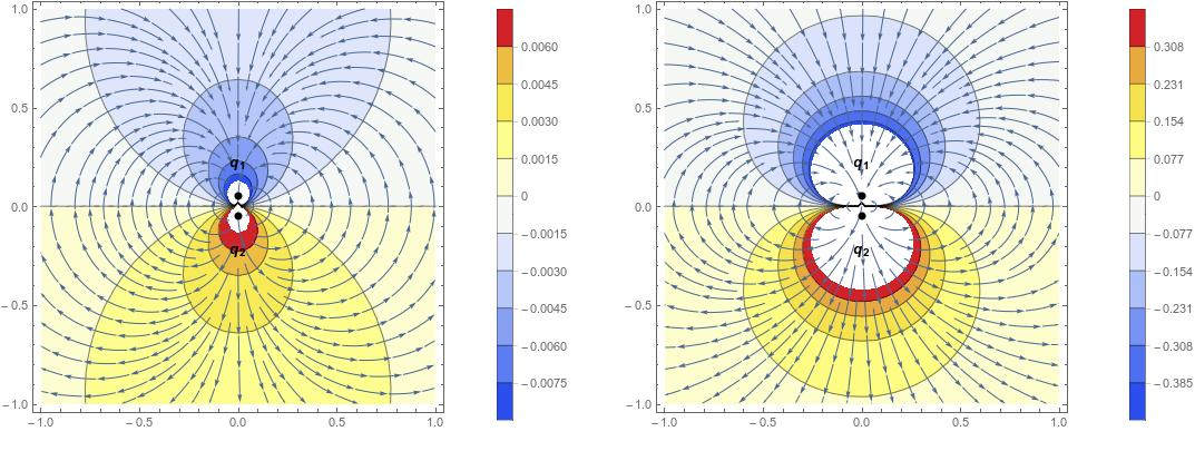
Figure 1: The left graph corresponds to the nonlinear dipole field, second term in Eq. (29); the right graph shows the standard dipole field. We use $R=0.05$, $q_{1}=-10$, $q_{2}=8$, $\gamma^{1/4}=40$. Besides the vast difference in the magnitude scale, the left pattern shows flattening towards the vertical axis, on which two bold dots indicating two charges are placed.

III.2 Large separation $r\ll R$ between charges

The quantities that relate to the approximation valid at $r\ll R,$ dealt with in this Subsection, will be supplied with tilde to be distinguished from the corresponding quantities in the previous Subsection III.1 relating to the opposite approximation.

Let us expand the inhomogeneity (23) to the first order in the ratio $\mathbf{r}/R$ (without assuming the smallness of $R$ and $r$ as compared to $\gamma^{1/4})$:

$$\mathbf{E}^{lin}\mathbf{(r})=\frac{q_{2}-q_{1}}{4\pi R^{2}}\frac{\mathbf{R}}{R}+\frac{\left(q_{2}+q_{1}\right)}{4\pi R^{2}}\left(\frac{\mathbf{r}}{R}-\frac{3\mathbf{R}}{R}\frac{\left(\mathbf{R\cdot r}\right)}{R^{2}}\right)+\dots$$ (31)

The first term here has a clear meaning of the sum of two oppositely directed Coulomb fields produced in the point $r=0$ by the two charges placed far from one another. The second one looks like a dipole field in the variable $R$ with the equivalent "dipole moment" $\left(q_{2}+q_{1}\right)\mathbf{r.}$

We are looking for solution to equation (22) in the form of the expansion in powers of $\mathbf{r}/R$

$$\mathbf{E}=\widetilde{\mathbf{E}}^{(0)}+\widetilde{\mathbf{E}}^{(1)}+\dots=\frac{f}{4\pi R^{2}}\frac{\mathbf{R}}{R}+\frac{1}{4\pi R^{2}}\left(\frac{\mathbf{r}}{R}c+\frac{\mathbf{R}}{R}\frac{\left(\mathbf{R\cdot r}\right)}{R^{2}}b\right)+\dots$$ (32)

with the the yet unknown dimensionless coefficients $f,$ $c$ and $b$ being functions of $R.$ The first Maxwell equation $\left[\mathbf{\nabla\times E}\right]=0$ is satisfied by (32).

In the zeroth order we have the equation for

$$\widetilde{\mathbf{E}}^{(0)}(R)=\frac{f}{4\pi R^{2}}\frac{\mathbf{R}}{R}=\widetilde{E}^{(0)}(R)\frac{\mathbf{R}}{R}$$

in form

$$\widetilde{E}^{(0)}\left(1+\frac{\gamma}{2}\widetilde{E}^{(0)2}\right)=\frac{q_{2}-q_{1}}{4\pi R^{2}},$$ (33)

which implies that $f/(4\pi R^{2})=\widetilde{E}^{(0)}(R)$ is the function obtained from $E^{(0)}(r)$ of the previous Subsection III.1 by the substitution $r\rightarrow R$ and $q_{2}+q_{1}\rightarrow q_{2}-q_{1}$.

III.2.1 Leading (dipole-like) approximation

In the first order, the use of (33) turns equation (22) to the linear algebraic equation for $\widetilde{\mathbf{E}}^{(1)}(R)$

$$\widetilde{\mathbf{E}}^{(1)}=\frac{\left(q_{2}+q_{1}\right)}{4\pi R^{2}}\left(\frac{\mathbf{r}}{R}-\frac{3\mathbf{R}}{R}\frac{\left(\mathbf{R\cdot r}\right)}{R^{2}}\right)-\frac{\gamma}{2}\left[2\left(\widetilde{\mathbf{E}}^{(1)}\cdot\widetilde{\mathbf{E}}^{(0)}\right)\widetilde{\mathbf{E}}^{(0)}+\widetilde{E}^{(0)2}\widetilde{\mathbf{E}}^{(1)}\right],$$ (34)

Calculating the second term in the right-hand side (the auxiliary electric field $\bm{\mathcal{E}}(\mathbf{r})=(\gamma/2)E^{2}(\mathbf{r})\mathbf{E}(\mathbf{r})$) with the ansatz (32)

$$2\left(\widetilde{\mathbf{E}}^{(1)}\cdot\widetilde{\mathbf{E}}^{(0)}\right)\widetilde{\mathbf{E}}^{(0)}+\widetilde{\mathbf{E}}^{(0)2}\widetilde{\mathbf{E}}^{(1)}=\frac{\mathbf{R}}{R}\widetilde{E}^{(0)2}\frac{\left(\mathbf{R\cdot r}\right)}{4\pi R^{4}}\left[2c+3b\right]+\mathbf{r}\widetilde{E}^{(0)2}\frac{c}{4\pi R^{3}},$$

we obtain from (34) two equations for the components of $\mathbf{E}^{(1)}$ along $\mathbf{R}$ and along $\mathbf{r}$ that determine the values

$$c=\frac{\left(q_{2}+q_{1}\right)}{1+\frac{\gamma}{2}\widetilde{E}^{(0)2}}=\frac{q_{2}+q_{1}}{q_{2}-q_{1}}\widetilde{E}^{(0)}R^{2},\quad b=-c\frac{3+\frac{5\gamma}{2}\widetilde{E}^{(0)2}}{1+\frac{3\gamma}{2}\widetilde{E}^{(0)2}}.$$

Finally

$$\mathbf{E} = \widetilde{\mathbf{E}}^{(0)}+\widetilde{\mathbf{E}}^{(1)}=$$ (35)

$$= \widetilde{E}^{(0)}(R)\frac{\mathbf{R}}{R}+\frac{q_{2}+q_{1}}{4\pi R^{2}\left(1+\frac{\gamma}{2}\widetilde{E}^{(0)2}(R)\right)}\left(\frac{\mathbf{r}}{R}-\frac{\mathbf{R}}{R}\frac{\left(\mathbf{R\cdot r}\right)}{R^{2}}\frac{3+\frac{5\gamma}{2}\widetilde{E}^{(0)2}(R)}{1+\frac{3\gamma}{2}\widetilde{E}^{(0)2}(R)}\right),$$

where $\widetilde{E}^{(0)}$ is the solution of equation (33) as a function of $R.$ The field (35) obviously satisfies the first Maxwell equation $\left[\mathbf{\nabla\times E}\right]=0.$ By comparing (35) with the linear field of two charges in the similar approximation (31) we observe that in the zero-order term, the difference $(q_{2}-q_{1})R^{-2}$ of the two Coulomb fields in the point $r=0$ has been replaced by the nonlinear field $\widetilde{E}^{(0)}$ of the equivalent charge $q_{2}-q_{1}$, while in the first-order term the "dipole field" $\left(q_{2}+q_{1}\right)\mathbf{r}$ has been modified by two different factors in the terms parallel to $\mathbf{r}$  and $\mathbf{R}.$

To be more general, note that the fields (35) and (29) turn into one another under the simultaneous replacement of the observation coordinate $r$ by the separation $R$ between charges, and of the sum $q_{2}+q_{1}$ of the charges by their difference $q_{2}-q_{1}.$ The same symmetry under the interchange $r\leftrightarrow R,$ $q_{2}+q_{1}\leftrightarrow q_{2}-q_{1}$ certainly holds for the linear $\gamma=0$ limits (31),(24) of Eqs. (35) and (29). This symmetry occurs, because the second Maxwell equations within the approximations adopted in this Subsubsection, $r\ll R,$ (34), and in the previous Subsection, $r\gg R,$ Eq. (26), turn into each other under the transformation under consideration, while the first Maxwell equation is satisfied for the both. As for the exact equation (22), this transformation maps it into a strange differential equation of a nonexisting theory.

III.2.2 Next-to-leading (quadrupole-like) approximation

In this Subsubsection we are studying the next, quadratic in the ratio $r/R$, term $\widetilde{\mathbf{E}}^{(2)}$ extending the expansion (32). To this end we first extend the expansion (31) of the linear field (23) $\mathbf{E}^{lin}(\mathbf{r})$ to include the corresponding term:

$$\mathbf{E}^{lin}(\mathbf{r})=\frac{q_{2}-q_{1}}{4\pi R^{2}}\frac{\mathbf{R}}{R}+\frac{q_{1}+q_{2}}{4\pi R^{2}}\left(\frac{\mathbf{r}}{R}-3\frac{\mathbf{R}}{R}\frac{(\mathbf{r}\cdot\mathbf{R})}{R^{2}}\right)+$$

$$+\frac{3(q_{1}-q_{2})}{8\pi R^{2}}\left(2\frac{(\mathbf{r}\cdot\mathbf{R})}{R^{2}}\frac{\mathbf{r}}{R}+\left(\frac{r}{R}\right)^{2}\frac{\mathbf{R}}{R}-5\frac{(\mathbf{r}\cdot\mathbf{R})^{2}}{R^{4}}\frac{\mathbf{R}}{R}\right)+O\left(\frac{r^{3}}{R^{3}}\right).$$ (36)

Once, up to the first order in $r/R$, Eq. (32) satisfies the first Maxwell equation $\left[\mathbf{\nabla\times E}\right]=0$ automatically with any coefficients $f,b,c$ we conclude, as we did in the previous Subsection, that the curl $[\mathbf{\nabla}\times\mathbf{\Omega}(\mathbf{r})]$ involved in (9) is zero to this order, Eq. (35) being the solution to equation (9) without this curl. This implies that the expansion of $[\mathbf{\nabla}\times\mathbf{\Omega}(\mathbf{r})]$ starts with the quadratic term $(r/R)^{2}$. Bearing in mind that the vector product $\left[\mathbf{r}\times\mathbf{R}\right]$ is the only pseudovector in our problem and that the action of $\mathbf{\nabla}$ lowers the power of $r$ by one we look for the pseudovector $\mathbf{\Omega}$ in the form

$$\mathbf{\Omega=}\frac{\left[\mathbf{r}\times\mathbf{R}\right]}{|\left[\mathbf{r}\times\mathbf{R}\right]|}\left[\Omega_{\phi}\left(\frac{\mathbf{r}\cdot\mathbf{R}}{rR}\right)\frac{r^{3}}{R^{3}}+O\left(\frac{r^{4}}{R^{4}}\right)\right],$$ (37)

where $\Omega_{\phi}\left((\mathbf{r}\cdot\mathbf{R})/(rR)\right)$ is a scalar function of the angle $\theta$ between the observation direction and the axis, on which the charges lie, $\cos\theta=(\mathbf{r}\cdot\mathbf{R})/(rR)$. The straightforward calculation yields (we refer to the orts $\mathbf{e}_{r}=\frac{\mathbf{r}}{r},\quad\mathbf{e}_{\phi}=-\frac{\mathbf{r}\times\mathbf{R}}{|\mathbf{r}\times\mathbf{R}|},\quad\mathbf{e}_{\theta}=\mathbf{e}_{\phi}\times\mathbf{e}_{r}$  and to the relation $\left(\nabla\cdot\mathbf{\Omega}\right)=0)$ obeyed by (37))

$$\left[\nabla\times\mathbf{\Omega}\right]=\frac{1}{R}\left[(\cot\theta\Omega_{\phi}(\theta)+\frac{d\Omega_{\phi}}{d\theta})\mathbf{e}_{r}-4\Omega_{\phi}(\theta)\mathbf{e}_{\theta}\right]\left(\frac{r}{R}\right)^{2},$$ (38)

$$\Delta\mathbf{\Omega=}-\left[\nabla\times\left[\nabla\times\mathbf{\Omega}\right]\right]=\frac{1}{R^{2}}\left(\frac{d^{2}\Omega_{\phi}(\theta)}{d\theta^{2}}+\cot\theta\frac{d\Omega_{\phi}(\theta)}{d\theta}-(\cot^{2}\theta-11)\Omega_{\phi}(\theta)\right)\frac{r}{R}\mathbf{e}_{\phi}.$$ (39)

From the last relation it follows that it is sufficient to solve equation (15) up to the first order in $r/R$. We expand the right-hand side of equation (15) in a series in $r/R$:

$$\mathbf{N}\times[(\mathbf{N}\cdot\vec{\nabla})\mathbf{N}]=\mathbf{E}^{lin}(\mathbf{r})\times\left((\mathbf{E}^{lin}(\mathbf{r})\cdot\nabla)(\mathbf{E}^{lin}(\mathbf{r})+\nabla\times\mathbf{\Omega})\right)+O\left(\frac{r}{R}\right)^{2}=$$ (40)

$$=\frac{(q_{1}-q_{2})^{2}}{16\pi^{2}R^{7}}\sin^{2}\theta\bigg{(}-\frac{d^{2}\Omega_{\phi}}{d\theta^{2}}+4\cot\theta\frac{d\Omega_{\phi}}{d\theta}+$$

$$+(3-6\csc^{2}\theta)\Omega_{\phi}-\frac{12q_{1}q_{2}}{4\pi R(q_{1}-q_{2})\sin\theta}\bigg{)}\frac{r}{R}\mathbf{e}_{\phi}+O\left(\frac{r}{R}\right)^{2},$$

$$2\frac{1-\xi\left(\gamma N^{2}\right)}{N^{2}}=\frac{8\pi R^{4}}{(q_{1}-q_{2})^{2}}\left(1-\kappa(R)\right)+O\left(\frac{r}{R}\right).$$ (41)

Thus, we obtain from (15) with the use of 39), (40) and (41) a linear differential equation for the function $\Omega_{\phi}(\theta)$:

$$\left(\kappa(R)-2-\left(\kappa(R)-1\right)\cos 2\theta\right)\frac{d^{2}\Omega_{\phi}(\theta)}{d\theta^{2}}-\left(4\left(\kappa(R)-1\right)\sin 2\theta+\cot\theta\right)\frac{d\Omega_{\phi}(\theta)}{d\theta}+$$

$$+\left(3\kappa(R)\left(\cos 2\theta+3\right)-3\left(\cos 2\theta+7\right)+\csc^{2}\theta\right)\Omega_{\phi}(\theta)=\frac{24q_{1}q_{2}(\kappa(R)-1)}{4\pi R(q_{2}-q_{1})}\sin\theta,$$ (42)

where $\kappa(R)=4\pi\tilde{E}^{(0)}R^{2}/(q_{2}-q_{1})=\xi\left(\gamma\frac{(q_{2}-q_{1})^{2}}{16\pi^{2}R^{4}}\right),$ and $\xi$ is the solution (12) of Eq. (11). The general solution of equation (42) in the class of functions regular in $\theta$ has the form:

$$\Omega_{\phi}(\theta)=\frac{12q_{1}q_{2}}{4\pi(q_{1}-q_{2})R}\frac{\kappa(R)-1}{3\kappa(R)-2}\sin\theta\cos^{2}\theta+C_{1}\sin\theta(1+7\cos(2\theta)+\frac{4}{\kappa(R)}\sin^{2}\theta).$$ (43)

The term with the constant $C_{1}$ satisfies the homogeneous equation obtained from (42) by omitting its right-hand side. Consequently, this solution determines a field that is not generated by the source, and therefore we discard it. The condition $C_{1}=0$ can be represented also in the form $\Omega_{\phi}\left(\pi/2\right)=0$. By substituting (43) with $C_{1}=0$ into (38) we have

$$\left[\nabla\times\mathbf{\Omega}\right]=\frac{24q_{1}q_{2}}{4\pi(q_{2}-q_{1})R^{2}}\frac{\kappa(R)-1}{2\kappa(R)-3}\frac{(\mathbf{r}\cdot\mathbf{R})}{R^{2}}\left(2\frac{(\mathbf{r}\cdot\mathbf{R})}{R^{2}}\frac{\mathbf{R}}{R}-\frac{\mathbf{r}}{R}\right)+O\left(\frac{r}{R}\right)^{3}.$$

Then

$$\mathbf{N}=\mathbf{E}^{lin}(\mathbf{r})+\nabla\times\mathbf{\Omega}=\mathbf{N}^{(0)}+\mathbf{N}^{(1)}+\mathbf{N}^{(2)}+O\left(\frac{r}{R}\right)^{3},$$

$$\mathbf{N}^{(0)}=\frac{q_{2}-q_{1}}{4\pi R^{2}}\frac{\mathbf{R}}{R},\quad\mathbf{N}^{(1)}=\frac{q_{1}+q_{2}}{4\pi R^{2}}\left(\frac{\mathbf{r}}{R}-3\frac{(\mathbf{r},\mathbf{R})}{R^{2}}\frac{\mathbf{R}}{R}\right),$$

$$\mathbf{N}^{(2)}=\frac{3(q_{1}-q_{2})}{8\pi R^{2}}\left[2\alpha(R)\frac{(\mathbf{r},\mathbf{R})}{R^{2}}\frac{\mathbf{r}}{R}+\left(\frac{r}{R}\right)^{2}\frac{\mathbf{R}}{R}-5\beta(R)\frac{(\mathbf{r},\mathbf{R})^{2}}{R^{4}}\frac{\mathbf{R}}{R}\right].$$

where

$$\alpha(R)=\frac{(q_{1}+q_{2})^{2}+\frac{4q_{1}q_{2}}{2\kappa(R)-3}}{(q_{1}-q_{2})^{2}},\quad\beta(R)=\frac{5(q_{1}^{2}+q_{2}^{2})+2q_{1}q_{2}\left(3+\frac{8}{2\kappa(R)-3}\right)}{5(q_{1}-q_{2})^{2}}.$$

For $N^{2}$ we have

$$N^{2}=N_{20}+N_{21}+N_{22}+O\left(\frac{r}{R}\right)^{3},$$

$$N_{20}=\frac{(q_{1}-q_{2})^{2}}{16\pi^{2}R^{4}},\quad N_{21}=\frac{q_{1}^{2}-q_{2}^{2}}{4\pi^{2}R^{4}}\frac{(\mathbf{r},\mathbf{R})}{R^{2}},$$

$$N_{22}=\frac{3}{4\pi^{2}R^{4}}\frac{(\mathbf{r},\mathbf{R})^{2}}{R^{4}}\left(q_{1}^{2}+q_{2}^{2}+q_{1}q_{2}\frac{2\kappa(R)-1}{2\kappa(R)-3}\right)-\frac{1}{8\pi^{2}R^{4}}(q_{1}^{2}+q_{2}^{2}-4q_{1}q_{2})\left(\frac{r}{R}\right)^{2}.$$

We expand expression (10) in series within the order $(r/R)^{2}$:

$$\mathbf{E}=\mathbf{N}\xi\left(\gamma N^{2}\right)=\mathbf{\tilde{E}}^{(0)}+\mathbf{\tilde{E}}^{(1)}+\mathbf{\tilde{E}}^{(2)}+O\left(\frac{r}{R}\right)^{3}.$$

The first two terms $\mathbf{\tilde{E}}^{(0)}$ and $\mathbf{\tilde{E}}^{(1)}$ are determined by the (35). For second-order correction $\mathbf{\tilde{E}}^{(2)}$ we obtain

$$\mathbf{\tilde{E}}^{(2)}=\xi\left(\gamma N_{20}\right)\mathbf{N}^{(2)}+\gamma N_{21}\xi^{\prime}\left(\gamma N_{20}\right)\mathbf{N}^{(1)}+\left(\gamma\xi^{\prime}\left(\gamma N_{20}\right)N_{22}+\frac{\gamma}{2}\xi^{\prime\prime}\left(\gamma N_{20}\right)N_{21}^{2}\right)\mathbf{N}^{(0)}.$$

Differentiating (11) we obtain expressions

$$\xi^{\prime}(x)=-\frac{\xi^{3}(x)}{2+3x\xi(x)^{2}},\quad\xi^{\prime\prime}(x)=12\frac{(1+x\xi^{2}(x))\xi^{5}(x)}{(2+3x\xi^{2}(x))^{3}}.$$

This finally results in the second-power correction to (35):

$$\widetilde{\mathbf{E}}^{(2)}=\frac{3}{8\pi R^{2}}\left(c(R)\left[2\frac{(\mathbf{r}\cdot\mathbf{R})}{R^{2}}\frac{\mathbf{r}}{R}+\frac{\mathbf{R}}{R}\left(\frac{r}{R}\right)^{2}\right]-5d(R)\frac{(\mathbf{r}\cdot\mathbf{R})^{2}}{R^{4}}\frac{\mathbf{R}}{R}\right),$$ (44)

where

$$c(R)=\frac{1}{3\kappa(R)}\left(\frac{(q_{1}+q_{2})^{2}}{q_{1}-q_{2}}+\frac{q_{1}^{2}-4q_{1}q_{2}+q_{2}^{2}}{q_{1}-q_{2}}\frac{2\kappa(R)}{3\kappa(R)-2}\right),$$

$$d(R)=\frac{\kappa(R)}{5(q_{1}-q_{2})(2\kappa(R)-3)}\bigg{(}8(q_{1}+q_{2})^{2}\kappa^{3}(R)-4(13(q_{1}^{2}+q_{2}^{2})+14q_{1}q_{2})\kappa^{2}(R)+$$

$$+2(47(q_{1}^{2}+q_{2}^{2})+14q_{1}q_{2})\kappa(R)-11(5(q_{1}^{2}+q_{2}^{2})-2q_{1}q_{2})\bigg{)}.$$

Note that (44) obeys the first Maxwell equation $\left[\nabla\times\widetilde{\mathbf{E}}^{(2)}\right]=0$ identically for any coefficients $c$ and $d$.

Similarly to the coefficient $(q_{1}-q_{2})$ in the third (quadrupole) term in (36), the coefficients $c(R)$ and $d(R)$ are odd under the permutation $q_{1}\leftrightarrow q_{2}.$ Note that the seeming singularity at $q_{1}=q_{2}$ cancels from these coefficients due to the equality $\kappa(R)=1$ that holds in this case. In the linear limit $\gamma=0$ one also has $\kappa(R)=1,$ and $c(R)$ and $d(R)$ turn both into $q_{1}-q_{2},$ so that (44) turns into the last (quadrupole) term in the expansion (36) of the linear field.

IV Concluding remarks

We were working within the simplest nonlinear electrodynamics with the self-interaction of the fourth power of electromagnetic field (5), which, if needed, may be thought of as resulting from the first nontrivial term of expansion of the Euler-Heisenberg effective Lagrangian in powers of its background field argument $\mathfrak{F}$, while the other field invariant is kept vanishing $\mathfrak{G=}0.$ In this case the coefficient $\gamma,$ whose dimensionality is [length${}^{4}],$ that determines the strength of nonlinearity is expressed as (6) in terms of the electron mass and charge. Otherwise it may be considered as arbitrary. Anyway, in our calculation a smallness of $\gamma^{1/4}$ as compared to the two other quantities $r$ and $R$ carrying the dimensionality of length was nowhere assumed.

We considered the electrostatic problem of interaction between two point-like charges $q_{1}$ and $q_{2}$ placed in the points $\mathbf{r}=\pm$ $\mathbf{R}$ by solving the nonlinear Maxwell equation (16), which follows from the least action principle for the Lagrangian (4), together with the standard Bianchi identity (8). For the small separation between the charges, $R\ll r,$ we found the electric field (29) in the approximation, linear with respect to the ratio $R/r$, which serves the nonlinear extension of the usual dipole field. The result for the corresponding scalar potential is Eq. (30). The lines-of-force and equipotential-curves pattern is shown in Fig. 1 in the configuration space $\mathbf{r}$ with the parameters chosen in such a way as to make the nonlinearity effect best pronounced. For large separation between the charges, $R\gg r,$ we found the electric field in the approximation, linear (35) with respect to the ratio $r/R$, and quadratic (44).

Using the two opposite reprentations (29) and (35) we can get a rough estimate for the behaviour of the field-energy (18), (17) in the asymptotic regime $R\rightarrow 0,$ where the two point charges approach each other infinitely close. According to that estimate, in this regime the energy of the system of two point charges can be presented as

$$P^{0}=a+bR^{\frac{1}{3}},$$ (45)

where $a$ and $b$ are finite constants depending only on the charges $q_{1}$ and $q_{2},$ and on the self-coupling constant $\gamma$. The $R$-independent term $a$ is the self-energy of the united point-like charge with the value $q_{1}+$ $q_{2}.$ This is finite, as established in CosGitSha2013a . The behaviour (45) is rigorously confirmed following a quite different procedure to be published elsewhere. Although the energy is finite in the limit $R=0,$ the force $\mathbf{F}$ between the two charges defined as the derivative of the energy with respect to the distance is weakly infinite:

$$\mathbf{F=}\frac{dP^{0}}{d\mathbf{R}}=\frac{\mathbf{R}}{R^{\frac{5}{3}}}\frac{b}{3}.$$

This formula replaces, in the given nonlinear model, the Coulomb law $\mathbf{F}\sim\mathbf{R}\cdot R^{-3}$ for the force between two point charges. The power $2/3$ here is determined by the power $2$ in the self-interaction in (5).

References

• (1) C.V. Costa, D.M. Gitman, A.E. Shabad, Finite field-energy of a point charge in QED, Phys. Scr. 90 (2015) 074012, http://stacks.iop.org/1402-4896/90/074012, arXiv:1312.0447 [hep-th] (2013).
• (2) T.C. Adorno, D.M. Gitman, A.E. Shabad and A. Shishmarev, Izvestiya Vusov, FIZIKA, 59, 45 (2016) (in Russian; translation: Russ. Phys. Journ., 59, 1775 (2017).
• (3) D.M. Gitman, A.E. Shabad and A. Shishmarev, Moving point charge as a soliton in nonlinear electrodynamics, arXiv:1509.0640[hep-th] (2015).
• (4) M.B. Ependiev, Teor. Mat. Fiz. 191, 417 (2017) (in Russian; translation: Theor. Math. Phys., 191, 836 (2017).
• (5) S.I. Kruglov, Mod. Phys. Lett. A23, 245 (2008).
• (6) S. Kruglov, Annals Phys. 383, 550 (2017); Notes on Born-Infeld-type electrodynamics, arXiv:1612.04195 (2016); Phys. Rev. D 94, 044026 (2016); Phys. Rev. D92 (2015) 12, 123523; Eur. Phys. J. C (2015) 75, 88 (2015); Phys. Rev. D 75, 117301 (2007). P. Gaete, J. Helayël-Neto, Eur. Phys. J. C 74, 2816 (2014).
• (7) M. Born and L. Infeld, Proc. Royal Soc. (London) A 144, 425 (1934).
• (8) S.H. Hendi, Ann. Phys. 333, 282 (2013). S.H. Hendi, S.Panahiyan and M. Momennia, Int. J. Mod. Phys. D 25, 2650063 (2016); S.H. Hendi, S.Panahiyan and R. Mamasani, Gen. Relativ. Gravit. 47, 91 (2015); L. Balart, Mod. Phys.Lett. A 24, 2777 (2009); Z. Dayyani, A. Sheykhi, M. H. Dehghani, Phys. Rev. D 95, 084004 (2017). M. Novello, J. M. Salim, A.N. Aranjo, Phys. Rev. D 85, 023528 (2012). M. Novello, S. E. Perez Bergliaffa and J. M. Salim, Phys. Rev. D 69, 127301 (2004). M. Novello, E. Goulart, J. M. Salim and S. E. Perez Bergliaffa, Class. Quant. Grav. 24, 3021 (2007). D. N. Vollick, Phys. Rev. D 78, 063524 (2008).
• (9) W. Heisenberg and H. Euler, Z. Phys. 98, 714 (1936); V. Weisskopf, Kong. Dans. Vid. Selsk. Math-fys. Medd. XIV, 6 (1936) (English translation in: Early Quantum Electrodynamics: A Source Book, A.I. Miller ( University Press, Cambridge, 1994).).
• (10) T.C. Adorno, D. M. Gitman, and A. E. Shabad,  Phys. Rev. D 93, 125031 (2016)).
• (11) D. M. Gitman and A. E. Shabad, Nonlinear (magnetic) corrections to the field of a static charge in an external field, Phys. Rev. D 86, 125028 (2012).
• (12) T.C. Adorno, D. M. Gitman, and A. E. Shabad, Magnetic response to applied electrostatic field in external magnetic field, Eur. Phys. J. C 74, 2838 (2014); Electric charge is a magnetic dipole when placed in a background magnetic field, Phys. Rev. D 89, 047504 (2014).
• (13) T.C. Adorno, D. M. Gitman, and A. E. Shabad, When an electric charge becomes also a magnetic one, Phys. Rev. D 92, 041702 (RC) (2015); also a paper under preparation.
• (14) C.V. Costa, D.M. Gitman, and A.E.Shabad, Nonlinear corrections in basic problems of electro- and magneto-statics in the vacuum, Phys. Rev. D 88, 085026 (2013).
• (15) B. King, P. Böhl and H. Ruhl, Phys. Rev. D 90, 065018 (2014).
• (16) D.M. Gitman, A.E. Shabad, and A.A. Shishmarev,  Phys. Scr. 92, 054005 (2017).
• (17) L.D. Landau, E.M. Lifshitz, The Classical Theory of Fields. (Addison-Wesley, Vol. 2 (1st ed.), 1951).
• (18) S. Weinberg, The Quantum Theory of Fields (University Press, Cambridge, 2001).
• (19) V.I. Ritus, in Problems of quantum electrodynamics of intense field, Trudy of P.N.Lebedev Phys. Inst. 168, 5 (1986).