On Stein’s Identity and Near-Optimal Estimation in High-dimensional Index Models

On Stein’s Identity and Near-Optimal Estimation in High-dimensional Index Models

Abstract

We consider estimating the parametric components of semi-parametric multiple index models in a high-dimensional and non-Gaussian setting. Such models form a rich class of non-linear models with applications to signal processing, machine learning and statistics. Our estimators leverage the score function based first and second-order Stein’s identities and do not require the covariates to satisfy Gaussian or elliptical symmetry assumptions common in the literature. Moreover, to handle score functions and responses that are heavy-tailed, our estimators are constructed via carefully thresholding their empirical counterparts. We show that our estimator achieves near-optimal statistical rate of convergence in several settings. We supplement our theoretical results via simulation experiments that confirm the theory.

1 Introduction

Consider the semi-parametric index model relating the response ($Y$) and the covariate ($X$) by

$$Y=f\left(\langle\beta^{*}_{1},X\rangle,\ldots,\langle\beta^{*}_{k},X\rangle\right)+\epsilon,$$ (1.1)

where $X,\{\beta_{\ell}^{*}\}_{\ell\in[k]}\in\mathbb{R}^{d}$ and $\epsilon$ is a zero-mean noise that is independent of $X$. Here the vectors $\{\beta^{*}_{\ell}\}_{\ell\in[k]}$ are the parametric components and the function $f$ is the nonparametric component or the link function. Such a model is called as multiple index model (MIM) in the literature. In this work, given $n$ i.i.d samples $\{X_{i},Y_{i}\}_{i=1}^{n}$ from the above model, where $n<d$, we are concerned with estimating the parametric components $\{\beta_{\ell}^{*}\}_{\ell\in[k]}$ when $f$ is unknown. More importantly, we do not impose the assumption that $X$ is Gaussian or elliptically symmetric, which is commonly made in the literature. Two important special cases of our model include phase retrieval (in which $k=1$), popular in signal processing, and sufficient dimensionality reduction (in which $k\geq 1$), popular in machine learning and statistics. Motivated by these applications, we make a distinction between the case of $k=1$, which is also called as single index model (SIM), and $k>1$ in the rest of the paper.

Estimating the parametric components $\{\beta_{\ell}^{*}\}_{\ell\in[k]}$ without depending on the exact form of the link function appears naturally in several situations. For example, in phase retrieval (Jaganathan et al., 2015), one-bit compressed sensing (Boufounos and Baraniuk, 2008) and sparse generalized linear models (Loh and Wainwright, 2015), we are interested in recovering a true parameter based on structured nonlinear measurements. In sufficient dimensionality reduction, where $k$ is typically a fixed number greater than one, but much less than $d$, we would like to estimate the projection onto the subspace spanned by the parametric components $\{\beta_{\ell}^{*}\}_{\ell\in[k]}$ without depending on the specific form of the function $f$. Furthermore, in deep neural networks (DNN), which are cascades of the MIM, the nonparametric component corresponds to the activation function which is pre-specified and the task is to estimate the parametric components, which are used for prediction in the test stage. Hence, it is crucial to develop estimators for the linear component with both statistical accuracy and computational efficiency for a wide class of link functions.

Several subtle issues arise when we consider optimal estimation in SIM and MIM. Specifically, most existing results depend crucially on the assumption made on $X$ or $f$ and fail to hold when those assumptions are relaxed. Such issues arise even in low-dimensional settings, where $n>d$. Consider, for example, the case of $k=1$ and a known link function $f(u)=u^{2}$. This corresponds to phase retrieval, which is a challenging inverse problem that has regained interest in the last few years along with the success of compressed sensing. A straightforward way to estimate $\beta^{*}$ is to do nonlinear least squares regression (Lecué and Mendelson, 2015), which is a nonconvex optimization problem. Candès et al. (2013) propose an estimator based on convex relaxations. Although their estimator is optimal when $X$ is sub-Gaussian, they are not agnostic to the link function, i.e., the same result does not hold if the link function is misspecified.

Direct optimization of the nonconvex phase retrieval problem was considered by Candes et al. (2015) and Sun et al. (2016), which propose estimators based on iterative algorithms that are statistical optimal. However, they rely on the assumption that $X$ is Gaussian. A careful look at their proofs reveal that extending them to a wider class of distributions is significantly challenging – for example, they require sharp concentration inequalities for polynomials of degree four of $X$, which would lead to suboptimal rate even when $X$ is sub-Gaussian. Furthermore, their results are not agnostic to the link function as well. Similar observations could be made for both convex (Li and Voroninski, 2013) and nonconvex estimators (Cai et al., 2015) for sparse phase retrieval in high dimensions. In addition, a surprising result for SIM was established in Plan and Vershynin (2016). They show that when $X$ is Gaussian, for a class of unknown link functions, one could estimate $\beta^{*}$ at the optimal statistical rate with the convex Lasso estimator. Unfortunately, their assumption on the link function is rather restrictive and rule out several interesting models including phase retrieval. Furthermore, none of the above procedures are applicable to the case of MIMs.

1.1 Motivation

Our work is primarily motivated by the interesting phenomenon illustrated in (Plan and Vershynin, 2016) for a class of high-dimensional SIM. Below, we first briefly summarize the result from (Plan and Vershynin, 2016) and then provide our alternative justification for the same result via Stein’s identity. We mainly leverage this alternative justification and propose our estimators for the more general setting we consider. Assuming, for simplicity, we work in the one-dimensional setting and are given $n$ i.i.d. samples from the SIM. Consider the least-squares estimator

$$\widehat{\beta}_{LS}=\underset{\beta\in\mathbb{R}}{\mathop{\mathrm{argmin}}}~{}~{}\frac{1}{n}\sum_{i=1}^{n}\left(Y_{i}-X_{i}\beta\right)^{2}.$$

Note that the above estimator is the standard least-squares estimator assuming a linear model (i.e., identity link function). The surprising observation from (Plan and Vershynin, 2016) is that, under the crucial assumption that $X$ is standard Gaussian, $\widehat{\beta}_{LS}$ is a good estimator of $\beta^{*}$ (up to a scaling) even when the data is generated from a nonlinear SIM. The same holds true for the high-dimensional setting when the minimization is performed in an appropriately constrained norm-ball (for example, the $\ell_{1}$-ball). Hence the theory developed for the linear setting could be leveraged to understand the performance in the SIM setting. Below, we give an alternative justification for the above estimator as an implication of Stein’s identity in the Gaussian case, which is summarized as follows.

Proposition 1.1 (Gaussian Stein’s Identity (Stein, 1972)).

Let $X\sim N(0,1)$ and $g:\mathbb{R}\to\mathbb{R}$ be a continuous function such that ${\mathbb{E}}|g^{\prime}(X)|\leq\infty$. Then we have ${\mathbb{E}}[g(X)X]={\mathbb{E}}[g^{\prime}(X)]$.

Note that in our context, if we let $g(X)=f(\langle X,\beta\rangle)$, then we have ${\mathbb{E}}[g^{\prime}(X)]\propto\beta^{*}$ and $\mathbb{E}[f(X)X]=\mathbb{E}[Y\cdot X]$. Now consider the following estimator, which is based on performing least-squares on the sample version of the above proposition:

$$\widehat{\beta}_{SL}=\underset{\beta\in\mathbb{R}}{\mathop{\mathrm{argmin}}}~{}~{}\frac{1}{n}\sum_{i=1}^{n}(Y_{i}X_{i}-\beta)^{2}$$

Note that $\widehat{\beta}_{LS}$ and $\widehat{\beta}_{SL}$ are the same estimators assuming $X\sim N(0,1)$, as $n\to\infty$. This observation leads to an alternative interpretation of the estimator proposed by (Plan and Vershynin, 2016) via Stein’s identity for Gaussian random variables. Thus it provides an alternative justification for why the linear least-squares estimator should work in the SIM setting. Interestingly, a similar procedure based on second-order Stein’s identity (see §2 for precise definitions) was used in Candes et al. (2015) to provide a favorable initializer for their gradient descent algorithm for phase retrieval. Our observation also provides an alternative interpretation of the initialization method used in Candes et al. (2015) by appealing to Stein’s identity. These observations also naturally leads to leveraging non-Gaussian versions of Stein’s identity for dealing with non-Gaussian covariates. Our estimators based on this motivation is described in detail in §3 and §4.

1.2 Related Work

The success of Lasso and related linear estimators in high-dimensions (Bühlmann and van de Geer, 2011), also enabled the exploration of high-dimensional SIMs. Although, this is very much work in progress. As mentioned previously, Plan and Vershynin (2016) show that the Lasso estimator works for the SIMs in high dimensions when the data is Gaussian. A more tighter albeit an asymptotic results under the same setting was proved in Thrampoulidis et al. (2015). Very recently Goldstein et al. (2016) extend the results of Li and Duan (1989) to the high dimensional setting but it suffers from similar problems as mentioned in the low-dimensional setting. Neykov et al. (2016) considered a misspecified phase retrieval model with Gaussian covariates and established rates of convergence. For the case of monotone nonparametric component, Yang et al. (2015) analyze a non-convex least squares approach under the assumption that the data is sub-Gaussian. However, the success of their method hinges on the knowledge of the link function. Furthermore, Jiang and Liu (2014); Lin et al. (2015); Zhu et al. (2006) analyze the sliced inverse regression estimator in the high-dimensional setting concentrating mainly on support recovery and consistency properties. Similar to the low-dimensional case, the assumptions made on the covariate distribution restrict them from several real-world applications involving non-Gaussian or non-symmetric covariate, for example high-dimensional problems in economics (Fan et al., 2011). Furthermore, several results are established on a case-by-case basis for fixed link function. Specifically Boufounos and Baraniuk (2008); Ai et al. (2014) and Davenport et al. (2014) consider 1-bit compressed sensing and matrix completion respectively, where the link is assumed to be the sign function. Also, Waldspurger et al. (2015) and Cai et al. (2015) propose and analyze convex and non-convex estimators for phase retrieval respectively, in which the link is the square function. All the above works, except Ai et al. (2014) make Gaussian assumptions on the data and are specialized for the specific link functions. The non-asymptotic result obtained in Ai et al. (2014) is under sub-Gaussian assumptions, but the estimator is not consistent. Finally, there is a line of work focusing on estimating both the parametric and the nonparametric component Kalai and Sastry (2009); Kakade et al. (2011); Alquier and Biau (2013); Radchenko (2015). We do not focus on this situation in this paper as mentioned before.

For multiple index models, relatively less work exist in the high-dimensional setting. In the low-dimensional setting, a line of work for estimation in MIMs is proposed by Ker-Chau Li, which include inverse regression (Li, 1991), principal Hessian directions (Li, 1992) and regression under link violation (Li and Duan, 1989). The proposed estimators are applicable for a class of unknown link functions under the assumption that the covariate follows a Gaussian or symmetric elliptical distribution. Such an assumption is restrictive as often times the covariates are heavy-tailed or skewed (Horowitz, 2009; Fan et al., 2011). Furthermore, they concentrate only on the low-dimensional setting establishing asymptotic statements. Estimation in high-dimensional MIM under the subspace sparsity assumption was considered in Chen et al. (2010), where the results are asymptotic and the proposed estimators are not computable in polynomial time.

To summarize, all the above works require restrictive assumption on either the data distribution or on the link function. We propose and analyze an estimator for a class of (unknown) link functions for the case when the covariates are drawn from a non-Gaussian distribution – under the assumption that we know the distribution a priori. Note that in several situations, one could fit specialized distributions, to real-world data that is often times skewed and heavy-tailed, so that it provides a good generative model of the data. Also, mixture of Gaussian distribution, with the number of components selected appropriately, approximates the set of all square integrable distributions to arbitrary accuracy (see for example McLachlan and Peel (2004)). Furthermore, since this is a density estimation problem it is unlabeled and there is no issue of label scarcity. Hence it is possible to get accurate estimate of the distribution in most situations of interest. Thus our work is complementary to the existing literature and provides an estimator for a class of models that is not addressed in the previous works.

1.3 Contributions

As discussed before, there are several subtleties based on the interplay between the assumptions made on $X$ and $f$ when dealing with estimation in SIM and MIM. Thus an interesting question is, whether it is possible to estimate the linear components in SIMs and MIMs with milder assumptions on both $X$ and $f$ in the high-dimensional setting. In this work, we provide a partial answer to this question. We construct estimators that work for a wide class of link functions, including the phase retrieval link function, and for a large family of distributions of $X$, which is assumed to be known a priori. We particularly focus on the case when $X$ follows a non-Gaussian distribution that need not be elliptically symmetric or sub-Gaussian, thus making our method applicable to several situations not possible before. Our estimators are based on Stein’s identity for non-Gaussian distributions, which utilizes the score function. Estimating with the score function is challenging due to their heavy tails. In order to illustrate that, consider the univariate histograms provided in Figure-1. The dark shaded, more concentrated one corresponds to the histogram of $10000$ samples from Gamma distribution with shape and scale parameters set to $5$ and $0.2$ respectively. The transparent histogram corresponds to the distribution of the score function of the same Gamma distribution. Note that even when the actual Gamma distribution is well concentrated, the distribution is the corresponding score function is well-spread and heavy-tailed. In the high dimensional setting, in order to estimate with the score functions, we require certain vectors or matrices based on the score functions to be well-concentrated in appropriate norms. In order to achieve that, we construct robust estimators via careful truncation arguments to balance the bias (due to thresholding)-variance (of the estimator) tradeoff and achieve the required concentration. In summary, our contribution are as follows:

• We construct estimators for the parametric component of a sparse SIM and MIM for a class of unknown link function under the assumption that the covariate distribution is non-Gaussian but known a priori. Our results are applicable for the case of vector, matrix or tensor valued covariates with appropriately defined structures to facilitate high-dimensional estimation.

• We establish near-optimal statistical rates for our estimators. Our results complement the existing ones in the literature and hold in several case not possible before.

• We provide alternative justifications based on the Stein’s identity for the estimator used in Plan and Vershynin (2016) for sparse SIM and the initializer used in Candes et al. (2015) for phase retrieval.

• As a consequence of our results for SIM and MIM, we also obtain a near-optimal estimator for sparse PCA with heavy-tailed data in the moderate sample size regime.

• We provide numerical simulations that confirm our theoretical results.

Parts of the results presented in this work, appeared in Yang et al. (2017a) and Yang et al. (2017b) previously.

Figure 1: Histogram of Score Function based on $10000$ independent samples from the Gamma distribution with shape $5$ and scale $0.2$. The dark histogram (we recommend the reader to zoom in to notice it) concentrated around zero corresponds to the Gamma distribution and the transparent histogram corresponds to the distribution of the score of the same Gamma distribution.

1.4 Notations

In this section, we introduce the notation and define the single index models. Throughout this work, we use $[n]$ to denote the set $\{1,\ldots,n\}$. In addition, for a vector $v\in\mathbb{R}^{d}$, we denote by $\|v\|_{p}$ the $\ell_{p}$-norm of $v$ for any $p\geq 1$. We use ${\mathcal{S}}^{d-1}$ to denote the unit sphere in $\mathbb{R}^{d}$, which is defined as ${\mathcal{S}}^{d-1}=\{v\in\mathbb{R}^{d}\colon\|v\|_{2}=1\}$. In addition, we define the support of $v\in\mathbb{R}^{d}$ as $\mathop{\text{supp}}(v)=\{j\in[d],v_{j}\neq 0\}$. Moreover, we denote the nuclear norm, operator norm, element-wise max norm and Frobenius norm of a matrix $A\in\mathbb{R}^{d_{1}\times d_{2}}$ by $\|\cdot\|_{\mathop{\star}}$, $\|\cdot\|_{\mathop{\text{op}}}$, $\|\cdot\|_{\infty}$ and $\|\cdot\|_{\mathop{\text{fro}}}$, respectively. We denote by $\mathop{\text{vec}}(A)$ the vectorization of matrix $A$, which is a vector in $\mathbb{R}^{d_{1}\cdot d_{2}}$. For two matrices $A,B\in\mathbb{R}^{d_{1}\times d_{2}}$ we define the trace inner product as $\langle A,B\rangle={\textsc{trace}}(A^{\top}B)$. Note that it can be viewed as the standard inner product between $\mathop{\text{vec}}(A)$ and $\mathop{\text{vec}}(B)$. In addition, for an univariate function $g\colon\mathbb{R}\rightarrow\mathbb{R}$, we denote by $g\circ(v)$ and $g\circ(A)$ the output of applying $g$ to each element of a vector $v$ and a matrix $A$, respectively. Finally, for a random variable $X\in\mathbb{R}$ with density $p$, we use $p^{\otimes d}\colon\mathbb{R}^{d}\rightarrow\mathbb{R}$ to denote the joint density of $\{X_{1},\cdots,X_{d}\}$, which are $d$ identical copies of $X$. We also require some notations about tensors. We concentrate on fourth-order tensors for simplicity. For any fourth-order tensor $Z\in\mathbb{R}^{d_{1}\times d_{2}\times d_{3}\times d_{4}}$, we denote its $(j_{1},j_{2},j_{3},j_{4})$-th entry by $Z(j_{1},j_{2},j_{3},j_{4})$. If $d_{\ell}=d$ for all $\ell\in[4]$, we denote the tensor as $Z\in\mathbb{R}^{d^{\otimes}4}$. Similar to the matrix case, we define $\mathop{\text{vec}}(Z)\in\mathbb{R}^{d^{4}}$ as the vectorization of the tensor $Z$. For two tensors $W,Z\in\mathbb{R}^{d^{\otimes}4}$, we define their inner inner product as

$$\langle Z,W\rangle =\mathop{\text{vec}}(Z)^{\top}\mathop{\text{vec}}(W)$$ (1.2)

$$=\sum_{j_{1},j_{2},j_{3},j_{4}\in[d]}Z(j_{1},j_{2},j_{3},j_{4})\cdot W(j_{1},j_{2},j_{3},j_{4})$$

The tensor Frobenius norm of is also denoted by $\|\cdot\|_{\mathop{\text{fro}}}$.

2 Index Models

Now we are ready to define the precise statistical models that we consider in this work. As mentioned above, we consider the case of $k=1$ (SIM) and $k>1$ (MIM) separately. We primarily distinguish our models based on the assumption made on the link functions. We also require the following definition of score function of random variable. Let $p\colon\mathbb{R}^{d}\rightarrow\mathbb{R}$ be a probability density function defined on $\mathbb{R}^{d}$. The score function $S_{p}\colon\mathbb{R}^{d}\rightarrow\mathbb{R}$ associated to density $p$ is defined as

$$S_{p}(x)=-\nabla_{x}[\log p(x)]=-\nabla_{x}p(x)/p(x).$$

Note that in the above definition, the derivative is taken with respect to $x$. This is different from the more traditional definition of the score function where the density belongs to a parametrized family and the derivative is taken with respect to the parameters. In the rest of the paper to simplify the notation, we omit the subscript $x$ from $\nabla_{x}$. We also omit the subscript $p$ from $S_{p}$ when the underlying density $p$ is clear from the context.

2.1 First-order Link Functions

We first discuss a class of SIM that are based on a certain first-order link functions. We discuss the motivation for our estimator, which automatically highlights the first-order assumption on the link function as well. Recall that our estimators are based on Stein’s identity. To begin with, we present the first-order non-Gaussian Stein’s identity.

Proposition 2.1 (First-order Stein’s Identity (Stein et al., 2004)).

Let $X\in\mathbb{R}^{d}$ be a real-valued random vector with density $p$. Assume that $p\colon\mathbb{R}^{d}\rightarrow\mathbb{R}$ is differentiable. In addition, let $g:\mathbb{R}^{d}\to\mathbb{R}$ be a continuous function such that $\mathbb{E}[\nabla g(X)]$ exists. Then it holds that

$$\mathbb{E}[g(X)\cdot S(X)]=\mathbb{E}[\nabla g(X)],$$

where $S(x)=-\nabla p(x)/p(x)$ is the score function of $p$.

One could apply the above Stein’s Identity to SIMs to obtain an estimate of $\beta^{*}$. To see this, note that when $X\sim N(0,I_{d})$ we have $S(x)=x$, $\forall x\in\mathbb{R}^{d}$. In this case, as $\mathbb{E}(\epsilon)=0$, we have

$$\mathbb{E}(Y\cdot X)=\mathbb{E}[f(\langle X,\beta^{*}\rangle)\cdot X]=\mathbb{E}[f^{\prime}(\langle X,\beta^{*}\rangle)]\cdot\beta^{*}.$$

Hence one could estimate $\beta^{*}$ based on estimating the moment $\mathbb{E}(Y\cdot X)$. This observation leads to the estimator proposed in Plan and Vershynin (2016). This motivates the following definition of SIM with first order link functions.

Definition 2.2 (Vector SIM with First-order Links).

Under this model, we assume that the response variable $Y\in\mathbb{R}$ and the covariate $X\in\mathbb{R}^{d}$ are linked via

$$Y=f(\langle X,\beta^{*}\rangle)+\epsilon,$$ (2.1)

where $f\colon\mathbb{R}\rightarrow\mathbb{R}$ is an unknown univariate function, $\beta^{*}\in\mathbb{R}^{d}$ is the parameter of interest, and $\epsilon\in\mathbb{R}$ is the exogenous random noise such that $\mathbb{E}(\epsilon)=0$. In addition, we assume that the entries of $X$ are i.i.d. random variables with density $p_{0}$ and that $\beta^{*}$ is $s^{*}$-sparse, that is, $\beta^{*}$ contains only $s^{*}$ nonzero entries such that $s^{*}\ll n\ll d$. Moreover, since the norm of $\beta^{*}$ can be absorbed in $f$, we further let $\|\beta^{*}\|_{2}=1$ for identifiability. Finally, we assume $f$ and $X$ are such that $\mathbb{E}[f^{\prime}(\langle X,\beta^{*}\rangle)]\neq 0$.

Note that the SIM depends only on covariate only via inner products. Hence it is natural to generalize it to the case of matrix and tensor valued covariates. To enable estimation in a high-dimensional setting, we enforce low-rank constraints that we describe below.

Definition 2.3 (Matrix SIM with First-order Links).

For the low-rank case SIM, we assume that $\beta^{*}\in\mathbb{R}^{d_{1}\times d_{2}}$ has rank $r^{*}\ll\min\{d_{1},d_{2}\}$. In this scenario, $X\in\mathbb{R}^{d_{1}\times d_{2}}$ and the inner product in (2.1) is $\langle X,\beta^{*}\rangle={\textsc{trace}}(X^{\top}\beta^{*}).$ For model identifiability, we further assume that $\|\beta^{*}\|_{\mathop{\text{fro}}}=1$, similar to the sparse case. Finally, we assume $f$ and $X$ are such that $\mathbb{E}[f^{\prime}(\langle X,\beta^{*}\rangle)]\neq 0$.

Before we lay out the first-order low-rank tensor single index model, we first introduce additional notation for tensors. Denote by $u\otimes v\otimes s\otimes t\in\mathbb{R}^{d^{\otimes}4}$ a rank-one tensor. The minimum value of $r$ such that the tensor $Z$ could be written as a summation of $r$ rank-one tensors, i.e., $Z=\sum_{j=1}^{r}u_{j}\otimes v_{j}\otimes s_{j}\otimes t_{j},$ is called as the CP-rank of the tensor, denoted by $\mathrm{rank}_{CP}(Z)=r$. We now describe the low-rank tensor model that we consider in this work.

Definition 2.4 (Tensor SIM with First-order Links).

For the low-rank Tensor SIM model, we assume that $\beta^{*}\in\mathbb{R}^{d^{\otimes 4}}$ and has CP-rank, $\mathrm{rank}_{CP}(\beta^{*})=r^{*}$. In this scenario, $X\in\mathbb{R}^{d^{\otimes 4}}$ and the inner product in (2.1) is understood as defined in (1.2). For model identifiability, we further assume that $\|\beta^{*}\|_{\mathop{\text{fro}}}=1$, similar to the matrix case. Finally, we assume $f$ and $X$ are such that $\mathbb{E}[f^{\prime}(\langle X,\beta^{*}\rangle)]\neq 0$.

2.2 Second-order Link Functions

In the above models, it is crucial that $\mathbb{E}[f^{\prime}(\langle X,\beta^{*}\rangle)]\neq 0$, for it to work. Such a restriction prevents it from being applicable to some widely used cases of SIM, for example, phase retrieval where $f$ is the quadratic function. This limitation of the first order Stein’s identity, motivates us to examine the second order Stein’s identity which is summarized below.

Proposition 2.5 (Second-order Stein’s Identity (Janzamin et al., 2014)).

Assume that the density of $X$ is twice differentiable. In addition, we define the second-order score function $T\colon\mathbb{R}^{d}\rightarrow\mathbb{R}^{d\times d}$ as

$$T(x)=\nabla^{2}p(x)/p(x).$$

Then, for any twice differentiable function $g:\mathbb{R}^{d}\rightarrow\mathbb{R}$ such that $\mathbb{E}[\nabla^{2}g(X)]$ exists, we have

$$\mathbb{E}\bigl{[}g(X)\cdot T(X)\bigr{]}=\mathbb{E}\bigl{[}\nabla^{2}g(X)\bigr{]}.$$ (2.2)

Back to the phase retrieval example, when $X\sim N(0,I_{d})$, the second order score function now becomes $T(x)=xx^{\top}-I_{d},$ $\forall x\in\mathbb{R}^{d}$. Setting $g(x)=\langle x,\beta^{*}\rangle^{2}$ in (2.2), we have

$$\mathbb{E}[g(X)\cdot T(X)] =\mathbb{E}[g(X)\cdot(XX^{\top}-I)]$$ (2.3)

$$=\mathbb{E}[\langle X,\beta^{*}\rangle^{2}\cdot(XX^{\top}-I)]=2\beta^{*}{\beta^{*}}^{\top}.$$

Thus for phase retrieval, one could extract $\pm\beta^{*}$ based on second order Stein’s identity even in the situation where the first order Stein’s identity fails. Indeed, (2.3) used in Candes et al. (2015) implicitly to provide a spectral initialization for the Wirtinger flow algorithm in the case of Gaussian phase retrieval. Here, we provided an alternative justification based on Stein’s identity, for why such an initializer works. Motivated by the this observation, we propose to use the second order Stein’s identity to estimate the parametric component of SIMs and MIMs with a class of unknown link functions with non-Gaussian covariates. The precise statistical models that we consider are defined as follows.

Definition 2.6 (Vector SIM with Second-order Links).

Under this model, we assume that the response variable $Y\in\mathbb{R}$ and the covariate $X\in\mathbb{R}^{d}$ are linked via

$$Y=f(\langle X,\beta^{*}\rangle)+\epsilon,$$ (2.4)

where $f\colon\mathbb{R}\rightarrow\mathbb{R}$ is an unknown univariate function, $\beta^{*}\in\mathbb{R}^{d}$ is the parameter of interest, and $\epsilon\in\mathbb{R}$ is the exogenous random noise such that $\mathbb{E}(\epsilon)=0$. In addition, we assume that the entries of $X$ are i.i.d. random variables with density $p_{0}$ and that $\beta^{*}$ is $s^{*}$-sparse, that is, $\beta^{*}$ contains only $s^{*}$ nonzero entries. Moreover, since the norm of $\beta^{*}$ can be absorbed in $f$, we further let $\|\beta^{*}\|_{2}=1$ for identifiability. Finally, we assume $f$ and $X$ are such that $\mathbb{E}[f^{\prime\prime}(\langle X,\beta^{*}\rangle)]>0$.

Note that in the definition of the SIMs, we require that $\mathbb{E}[f^{\prime\prime}(\langle X,\beta^{*}\rangle)]$ positive. Since if $\mathbb{E}[f^{\prime\prime}(\langle X,\beta^{*}\rangle)]$ is negative , we could always replace $f$ by $-f$ by flipping the sign of $Y$, we essentially assume that $\mathbb{E}[f^{\prime\prime}(\langle X,\beta^{*}\rangle)]$ is nonzero. Intuitively, such restriction on $f$ implies that the second order moments contains the information of $\beta^{*}$, thus we call such a function the second order link. Similar to the first-order case, one could define matrix and tensor versions of the second-order SIMs but we do not concentrate on such models in this work. Thus far, we considered SIMs. We now define a class of MIMs with second order links. For MIMs the notion of first order link functions is naturally not sufficient to estimate the projector onto the subspace.

Definition 2.7 (MIM with Second-order Links).

Under this model, we assume that the response variable $Y\in\mathbb{R}$ and the covariate $X\in\mathbb{R}^{d}$ are linked via

$$Y=f\left(\langle X,\beta^{*}_{1}\rangle,\ldots,\langle X,\beta^{*}_{k}\rangle\right)+\epsilon,$$ (2.5)

where $f\colon\mathbb{R}^{k}\rightarrow\mathbb{R}$ is an unknown function, $\{\beta^{*}_{\ell}\}_{\ell\in[k]}\subseteq\mathbb{R}^{d}$ are the parameters of interest, and $\epsilon\in\mathbb{R}$ is the exogenous random noise such that $\mathbb{E}(\epsilon)=0$. In addition, we assume that the entries of $X$ are i.i.d. random variables with density $p_{0}$ and that $\{\beta^{*}_{\ell}\}_{\ell\in[k]}$ span a $k$-dimensional subspace of $\mathbb{R}^{d}$. Moreover, we denote $B^{*}=(\beta^{*}_{1}\ldots\beta^{*}_{k})\in\mathbb{R}^{d\times k}$. Then the model in (2.5) can be written as $Y=f(XB^{*})+\epsilon$. By the QR-factorization, we can write $B^{*}$ as $Q^{*}R^{*}$, where $Q^{*}\in\mathbb{R}^{d\times k}$ is an orthonormal matrix and $R^{*}\in\mathbb{R}^{k\times k}$ is invertible. Since $f$ is unknown, $R^{*}$ can be absorbed into the link function. Thus, we assume that $B^{*}$ is orthonormal for identifiability. Furthermore, we further assume that $B^{*}$ is $s^{*}$-row sparse, that is, $B^{*}$ contains only $s^{*}$ nonzero rows. We note that such a definition of sparsity for $B^{*}$ does not depends on the choice of coordinate system. Finally, we assume $f$ and $X$ are such that $\lambda_{\min}\left(\mathbb{E}[\nabla^{2}f(XB^{*})]\right)>0$.

The assumption $\mathbb{E}[\nabla^{2}f(XB^{*})]$ is positive definite, in MIM, is a multivariate generalization of the condition that $\mathbb{E}[f^{\prime\prime}(\langle X,\beta^{*}\rangle)]>0$ in SIM. It essentially guarantees that estimation of the projector onto the subspace spanned by the $k$ components is well-defined. We now introduce our estimators and provide theoretical results that are near-optimal in several settings.

3 Theoretical Results for Index Models with First-order Links

Recall that in the single index models introduced in §2.1, $X$ in (2.1) has i.i.d. entries with density $p_{0}$. To unify the vector, matrix and tensor settings, we identify $X$ with $\mathop{\text{vec}}(X)\in\mathbb{R}^{d}$ where $d=d_{1}\cdot d_{2}\cdot d_{3}\cdot d_{4}$. In this case, $X$ has density $p=p_{0}^{\otimes d}$ and the corresponding score function $S\colon\mathbb{R}^{d}\rightarrow\mathbb{R}^{d}$ is given by

$$S(x)=-\nabla\log p(x)=-\nabla p(x)/p(x)=s_{0}\circ(x),$$ (3.1)

where the univariate function $s_{0}=-p_{0}^{\prime}/p_{0}$ is applied to each entry of $x$. Thus $S(X)$ has i.i.d. entries. In addition, by Proposition 2.1, we have $\mathbb{E}[S(X)]=0$ by setting $g$ to be a constant function. Moreover, in the context of SIMs specified in (2.1), we have

$$\mathbb{E}[Y\cdot S(X)] =\mathbb{E}\bigl{[}f(\langle X,\beta^{*}\rangle)\cdot S(X)\bigr{]}$$

$$=\mathbb{E}[f^{\prime}(\langle X,\beta^{*}\rangle)]\cdot\beta^{*},$$

as long as the density and the link function satisfy the conditions stated in Proposition 2.1. This implies that optimization problem

$$\mathop{\mathrm{minimize}}_{\beta\in\mathbb{R}^{d}}\bigl{\{}\langle\beta,\beta\rangle-2\mathbb{E}[Y\cdot\langle S(X),\beta\rangle]\bigr{\}}$$ (3.2)

has solution $\beta=\mu\cdot\beta^{*}$, where $\mu=\mathbb{E}[f^{\prime}(\langle X,\beta^{*}\rangle)]$. Hence the above program could be used to obtain the unknown $\beta^{*}$ as long as $\mu\neq 0$. Before we proceed to describe the sample version of the above program, we make the following brief remark. The requirement $\mu\neq 0$ rules out in particular the use of our approach for non-Gaussian phase retrieval (where $f(u)=u^{2}$) as in that case we have $\mu=0$ when $X$ is centered. But we emphasize that the same holds true in the Gaussian and elliptical setting as well, as noted in Plan and Vershynin (2016) and Goldstein et al. (2016). Their methods also fail to recover the true $\beta^{*}$ when the SIM model corresponds to phase retrieval. We refer the reader to §4 for overcoming this limitation using second-order Stein’s identity.

We use a sample version of the above program as an estimator for the unknown $\beta^{*}$. In order to deal with the high-dimensional setting, we consider a regularized version of the above formulation. More specifically, we use the $\ell_{1}$-norm and nuclear norm regularization in the vector and matrix/tensor settings respectively. However, a major difficulty in the sample setting for this procedure is that $\mathbb{E}[Y\cdot S(X)]$ and its empirical counterpart may not be close enough due to a lack of concentration. Recall our discussion from §1 that even if the random variable $X$ is light-tailed, its score-function $S(x)$ might be arbitrarily heavy-tailed. Furthermore, bounded-fourth moment assumption on the noise, $Y$ too can be heavy-tailed. Thus the naive method of using the sample version of (3.2) to estimate $\beta^{*}$ leads to sub-optimal statistical rates of convergence.

To improve concentration and obtain optimal rates of convergence, we replace $Y\cdot S(X)$ with a transformed random variable ${\mathcal{T}}(Y,X)$, which will be defined precisely later for the sparse and low-rank cases. In particular, ${\mathcal{T}}(Y,X)$ is a carefully truncated version of $Y\cdot S(X)$, introduced and analyzed in Catoni et al. (2012); Fan et al. (2016) for related problems, that enables us to obtain well-concentrated estimators. Thus our final estimator $\widehat{\beta}$ is defined as the solution to the following regularized optimization problem

$$\mathop{\mathrm{minimize}}_{\beta\in\mathbb{R}^{d}}~{}L(\beta)+\lambda\cdot R(\beta),$$ (3.3)

where

$$L(\beta)=\langle\beta,\beta\rangle-\frac{2}{n}\sum_{i=1}^{n}\langle{\mathcal{T}}(Y_{i},X_{i}),\beta\bigr{\rangle},$$ (3.4)

and $\lambda>0$ is the regularization parameter which will be specified later and $R(\cdot)$ is the $\ell_{1}$-norm in the vector case and the nuclear norm in the matrix/tensor case. We now introduce our main moment assumption for first-order SIM. This assumption is made apart from the assumptions made on the noise and the link function. Recall that each entry of the score function defined in (3.1) is equal to $s_{0}(u)=-p_{0}^{\prime}(u)/p_{0}(u)$. We first state the assumption and make a few remarks about it.

Assumption 3.1 (Moment Assumptions).

There exists an absolute constant $M>0$ such that $\mathbb{E}(Y^{4})\leq M$ and $\mathbb{E}_{p_{0}}[s^{4}_{0}(U)]\leq M$, where random variable $U\in\mathbb{R}$ has density $p_{0}$.

Consider the assumption $\mathbb{E}(Y^{4})\leq M$. By Cauchy-Schwarz inequality we have $\mathbb{E}(Y^{4})\leq 4\mathbb{E}(\epsilon^{4})+4\mathbb{E}[f^{4}(\langle X,\beta^{*})]$. Note that we assume $\epsilon$ to be centered, independent of $X$ and has bounded fourth moment (see §2). If the covariate $X$ has bounded fourth moment along the direction of true parameter, since $f(\cdot)$ is continuously differentiable, $f(\langle X,\beta^{*}\rangle)$ has bounded fourth moment as well if $f(\cdot)$ is defined on a compact subset of $\mathbb{R}$. . Hence the condition $\mathbb{E}(Y^{4})\leq M$ is relatively easy to satisfy and significantly milder than assuming that $Y$ is bounded or has lighter tails. Furthermore, $\mathbb{E}_{p_{0}}[s^{4}_{0}(U)]\leq M$ is relatively mild and satisfied by a wide class of random variables. Specifically random variables that are non-symmetric and non-Gaussian satisfy this property thereby allowing our approach to work with covariates not previously possible. We believe it is highly non-trivial to weaken this condition without losing significantly in the rates of convergence that we discuss below.

3.1 Sparse Vector SIM

Under the above assumptions, we first state our theorem on the sparse SIM. As discussed above, $Y\cdot S(X)$ can by heavy-tailed and hence we apply truncation to achieve concentration. Denote the $j$-th entry of the score function $S$ in (3.1) as $S_{j}\colon\mathbb{R}^{d}\rightarrow\mathbb{R}$, $j\in[d]$. We define the truncated response and score function as

$$\widetilde{Y} =\mathop{\text{sign}}(Y)\cdot(|Y|\wedge\tau),$$ (3.5)

$$S_{j}(x) =\mathop{\text{sign}}[S_{j}(x)]\cdot\bigl{[}|S_{j}(x)|\wedge\tau\bigr{]},$$

where $\tau>0$ is a predetermined threshold value. We define $\widetilde{Y}_{i}$ similarly for all $Y_{i}$, $i\in[n]$. Then we define the estimator $\widehat{\beta}$ as the solution to the optimization problem in (3.3) with ${\mathcal{T}}(Y_{i},X_{i})=\widetilde{Y}_{i}\cdot\widetilde{S}(X_{i})$ and $R(\beta)=\|\beta\|_{1}$. Here we apply elementwise truncation in ${\mathcal{T}}$ to ensure the sample average of ${\mathcal{T}}$ converges to $\mathbb{E}[Y\cdot S(X)]$ in the $\ell_{\infty}$-norm for an appropriately chosen $\tau$. Note that the $\ell_{\infty}$-norm is the dual norm of the $\ell_{1}$-norm. Such a convergence requirement in the dual norm is standard in the analysis of regularized $M$-estimators (Negahban et al., 2012) to achieve optimal rates. The following theorem characterizes the convergence rates of $\widehat{\beta}$.

Theorem 3.2 (Signal Recovery for Sparse Vector SIM).

For the sparse SIM defined in §2, we assume that $\beta^{*}\in\mathbb{R}^{d}$ has $s^{*}$ nonzero entries. Under Assumption 3.1, we let

$$\tau=2(M\cdot\log d/n)^{1/4}$$

in (3.5) and set the regularization parameter $\lambda$ in (3.3) as

$$\lambda=C\sqrt{M\cdot\log d/n},$$

where $C>0$ is an absolute constant. Then with probability at least $1-d^{-2}$, the $\ell_{1}$-regularized estimator $\widehat{\beta}$ defined in (3.3) satisfies

$$\|\widehat{\beta}-\mu\beta^{*}\|_{2}\leq\sqrt{s^{*}}\cdot\lambda,~{}~{}\|\widehat{\beta}-\mu\beta^{*}\|_{1}\leq 4s^{*}\cdot\lambda.$$

From this theorem, the $\ell_{1}$- and $\ell_{2}$-convergence rates of $\widehat{\beta}$ are $\|\widehat{\beta}-\mu\beta^{*}\|_{1}=\mathcal{O}(s^{*}\sqrt{\log d/n})$ and $\|\widehat{\beta}-\mu\beta^{*}\|_{2}=\mathcal{O}(\sqrt{s^{*}\log d/n})$, respectively. These rates match the convergence rates of sparse generalized linear models (Loh and Wainwright, 2015) and sparse single index models with Gaussian and symmetric elliptical covariates (Plan and Vershynin, 2016; Goldstein et al., 2016) which are known to be minimax-optimal for this problem via matching lower bounds.

3.2 Low-rank Matrix SIM

We next state our theorem for the low-rank Matrix SIM. In this case, we apply the nuclear norm regularization to promote low-rankness. Note that by definition, ${\mathcal{T}}$ is matrix-valued. Since the dual norm of the nuclear norm is the operator norm, we need the sample average of ${\mathcal{T}}$ to converge to $\mathbb{E}[Y\cdot S(X)]$ in the operator norm rapidly to achieve optimal rates of convergence. To achieve such a goal, we leverage the truncation argument from Catoni et al. (2012); Minsker (2016); Fan et al. (2016) to construct ${\mathcal{T}}(Y,X)$.

Let $\phi\colon\mathbb{R}\rightarrow\mathbb{R}$ be a non-decreasing function such that

$$-\log(1-x+x^{2}/2)\leq\phi(x)\leq\log(1+x+x^{2}/2),~{}~{}\forall x\in\mathbb{R}.$$

Based on $\phi$, we define a linear mapping $\psi\colon\mathbb{R}^{d_{1}\times d_{2}}\rightarrow\mathbb{R}^{d_{1}\times d_{2}}$ as follows. For any $A\in\mathbb{R}^{d_{1}\times d_{2}}$, let

$$\widetilde{A}=\begin{bmatrix}0&A\\ A^{\top}&0\end{bmatrix}$$

and let $\Upsilon\Lambda\Upsilon^{\top}$ be the eigenvalue composition of $\widetilde{A}$. In addition, let $B=\Upsilon\bigl{[}\psi\circ(\Lambda)\bigr{]}\Upsilon^{\top}$, where $\psi$ is applied elementwisely on $\Lambda$. Then we write $B$ in block from as

$$B=\begin{bmatrix}B_{11}&B_{12}\\ B_{21}&B_{22}\end{bmatrix}$$

and define $\psi(A)=B_{12}$. Finally, we define ${\mathcal{T}}(Y,X)=1/\kappa\cdot\psi\bigl{[}\kappa\cdot Y\cdot S(X)\bigr{]},$ where $\kappa>0$ will be specified later. Therefore, our final estimator $\widehat{\beta}\in\mathbb{R}^{d_{1}\times d_{2}}$ is defined as the solution to the optimization problem in (3.3) with $R(\beta)=\|\beta\|_{\mathop{\star}}$. We note here the minimization in (3.3) is taken over $\mathbb{R}^{d_{1}\times d_{2}}$. The following theorem quantifies the convergence rates of the proposed estimator.

Theorem 3.3 (Signal Recovery for Low-rank Matrix SIM).

For the low-rank single index model defined in §2, we assume that $\mathrm{rank}(\beta^{*})=r^{*}$. Under Assumption 3.1, we let

$$\kappa=2\sqrt{n\cdot\log(d_{1}+d_{2})}/\sqrt{(d_{1}+d_{2})M}$$

in ${\mathcal{T}}(Y,X)$ and set $\lambda$ in (3.3) as

$$\lambda=C\sqrt{M\cdot(d_{1}+d_{2})\cdot\log(d_{1}+d_{2})/n},$$

where $C>0$ is an absolute constant. Then with probability at least $1-(d_{1}+d_{2})^{-2}$, the nuclear norm regularized estimator $\widehat{\beta}$ satisfies

$$\|\widehat{\beta}-\mu\beta^{*}\|_{\mathop{\text{fro}}}\leq 3\sqrt{r^{*}}\cdot\lambda,~{}~{}\|\widehat{\beta}-\mu\beta^{*}\|_{\mathop{\star}}\leq 12r^{*}\cdot\lambda.$$

By this theorem, we have $\|\widehat{\beta}-\mu\beta^{*}\|_{\mathop{\text{fro}}}=\mathcal{O}(\sqrt{r^{*}(d_{1}+d_{2})\cdot\log(d_{1}+d_{2})/n})$ and $\|\widehat{\beta}-\mu\beta^{*}\|_{\mathop{\star}}=\mathcal{O}(r^{*}\cdot\sqrt{(d_{1}+d_{2})\cdot\log(d_{1}+d_{2})/n})$. Note that the rate obtained is minimax-optimal up to a logarithmic factor. Furthermore, it matches the rates for low-rank single index models with Gaussian and symmetric elliptical distributions up to a logarithmic factor Plan and Vershynin (2016); Goldstein et al. (2016).

3.3 Low-rank Tensor SIM

We now state our result for low-rank tensor SIM. The notion of rank of a tensor is more delicate compared to that of a matrix. Several generalizations of the matrix rank exist for the case of tensors. Recall from Definition 2.4, that we assumed that the structure on $\beta^{*}$ is that it has low CP-rank. Unfortunately, enforcing such a constraint via a direct tensor nuclear norm relaxation (similar to that of the matrix nuclear norm) is NP-hard (Friedland and Lim, 2014).

One way to overcome such a computational hurdle is to deal with tensors via appropriately matricized forms. In order to enable computable estimators, we specifically leverage the results of Mu et al. (2014) and define the following square-unfolding of a tensor. Denote by $\mathop{\textrm{Mat}}\colon\mathbb{R}^{d^{\otimes}4}\rightarrow\mathbb{R}^{d^{2}\times d^{2}}$ the operation of tensor square-unfolding, which maps a fourth-order tensor to a square matrix. More specifically, the entries of $\mathop{\textrm{Mat}}(Z)$ are specified by $[\mathop{\textrm{Mat}}(Z)]_{k_{1},k_{2}}=Z(j_{1},j_{2},j_{3},j_{4}),$ where the indices satisfy the relationship $k_{1}=1+(j_{1}-1)+(j_{2}-1)\cdot d$ and $k_{2}=1+(j_{3}-1)+(j_{4}-1)\cdot d$. Intuitively, the matrix obtained by the square-unfolding operation is as square as possible, i.e., it is $d^{2}\times d^{2}$ rather than the rectangular $d\times d^{3}$ or $d^{3}\times d$ matrices. It is shown in Mu et al. (2014) such a square matricization preserves the low CP-rank of the original tensor. Hence one could use the matrix nuclear norm relaxation on the square-unfolded tensor. Furthermore, for the case of tensor SIM as in Definition 2.4, note that we have $\langle X,\beta^{*}\rangle=\langle\mathop{\textrm{Mat}}(X),\mathop{\textrm{Mat}}(\beta^{*})\rangle$. Combining the above observations, the low CP-rank tensor SIM problem could be reduced to that of low-rank matrix SIM problem, where matrix low-rank constraint, via nuclear norm, is enforced on $\mathop{\textrm{Mat}}(\beta^{*})$. Thus, we use the estimator in (3.3) with $R(\beta)=\|\mathop{\textrm{Mat}}(\beta)\|_{*}$ and $\mathop{\textrm{Mat}}(X_{i})$ for all $i=1,\ldots,n$ along with the truncation operation $\mathcal{T}$ described in §3.2. We now have the following theorem for the low-rank tensor SIM.

Theorem 3.4 (Signal Recovery for Low-rank Tensor SIM).

For the low-rank tensor single index model defined in §2, Definition 2.4, we assume that $\mathrm{rank}_{CP}(\beta^{*})=r^{*}$. Under Assumption 3.1, we let

$$\kappa=2\sqrt{2n\cdot\log d}/\sqrt{(2d^{2})M}$$

in ${\mathcal{T}}(Y,X)$ and set $\lambda$ in (3.3) as

$$\lambda=C\sqrt{2M\cdot(2d^{2})\cdot\log d/n},$$

where $C>0$ is an absolute constant. Then with probability at least $1-(2d)^{-2}$, the nuclear-norm regularized estimator $\widehat{\beta}$ satisfies

$$\|\widehat{\beta}-\mu\mathop{\textrm{Mat}}(\beta^{*})\|_{\mathop{\text{fro}}}\leq 3\sqrt{r^{*}}\cdot\lambda$$

We omit the proof of the above theorem as it is follows the exact steps of Theorem 3.3 proved in Appendix A.2. From the above theorem, we see that as long as $n=\Omega(r^{*}d^{2})$, we achieve consistent estimation of $\beta^{*}$ up to scaling. This improves upon recent results established in Chen et al. (2016), that established similar results under restrictive Gaussian covariate assumption and required knowledge of the link functions (i.e., generalized linear models). Furthermore our results significantly generalizes the results of Mu et al. (2014) that considered only linear link functions. Finally, although our structure on $\beta^{*}$ was a low CP-rank structure, the square matricization technique also applies for the case of low Tucker-rank, which is yet another notion of rank for tensors with several applications. It is straightforward to extend our results to this case of low Tucker-rank.

4 Theoretical Results for Index Models with Second-Order Links

We now introduce our estimators and establish their statistical rates of convergence for the case of index models with second-order link functions. Discussions on optimality of the established rates and connection to sparse PCA problem is deferred to §4.3. Similar to the first-order case, we focus on the case where $X$ has i.i.d. entries with density $p_{0}\colon\mathbb{R}\rightarrow\mathbb{R}$. Thus the joint density of $X$ is $p(x)=p_{0}^{\otimes d}(x)=\prod_{j=1}^{d}p_{0}(x_{j})$. We define a univariate function $s_{0}\colon\mathbb{R}\rightarrow\mathbb{R}$ by $s_{0}(u)=-p_{0}^{\prime}(u)/p_{0}(u)$. Then the first-order score function associated with $p$ is given by $S(x)=s_{0}\circ(x)$. Equivalently, the $j$-th entry of the first-order score function associated with $p$ is given by $[S(x)]_{j}=s_{0}(x_{j})$. Moreover, the second order score function is

$$T(x) =S(x)S^{\top}(x)-\nabla S(x)$$ (4.1)

$$=S(x)S^{\top}(x)-{\rm diag}[s_{0}^{\prime}\circ(x)].$$

Before we present our estimator, we introduce the assumption on $Y$ and $s_{0}(\cdot)$.

Assumption 4.1 (Moment Assumptions).

We assume that there exists a constant $M$ such that $\mathbb{E}_{p_{0}}[s_{0}^{6}(U)]\leq M$ and $\mathbb{E}(Y^{6})\leq M$. We denote $\sigma_{0}^{2}=\mathbb{E}_{p_{0}}[s_{0}^{2}(U)]=\operatorname{{\rm Var}}_{p_{0}}[s_{0}(U)]$.

The assumption that $\mathbb{E}_{p_{0}}[s_{0}^{6}(U)]\leq M$ allows wide family of distributions of including Gaussian and more heavy-tailed random variables. Furthermore, we do not require the covariate to be elliptically symmetric as is commonly seen in prior work, which enables our method to be applicable for skewed covariates. As for the assumption that $\mathbb{E}(Y^{6})\leq M$, in the case of SIMs, we have $\mathbb{E}(Y^{6})\leq C\left(\mathbb{E}(\epsilon^{6})+\mathbb{E}[f^{6}(\langle X,\beta^{*}\rangle)]\right)$. Thus this assumption is satisfied as long as both $\epsilon$ and $f(\langle X,\beta^{*}\rangle)$ have bounded sixth moments. This is a significantly milder assumption which allows for heavy-tailed response as opposed to bounded or light-tailed response.

4.1 Sparse Vector SIM

Now we are ready to describe our estimator for the sparse SIMs in Definition 2.6. Note that by Proposition 2.5 we have

$$\mathbb{E}\bigl{[}Y\cdot T(X)\bigr{]}=C_{0}\cdot\beta^{*}{\beta^{*}}^{\top},$$ (4.2)

where $C_{0}=2\mathbb{E}[f^{\prime\prime}(\langle X,\beta^{*}\rangle)]>0$ as per Definition 2.6. Therefore, one way to estimator $\beta^{*}$ is to obtain the leading eigenvector of $\mathbb{E}[Y\cdot T(X)]$ from the samples. Since $\beta^{*}$ is sparse, we formulate our estimator as a sparsity constrained semi-definite program:

$$\textrm{maximize}~{}~{}\langle W,\Sigma^{*}\rangle-\lambda\|W\|_{1}$$

$$\text{subject to}~{}~{}0\preceq W\preceq I_{d},~{}~{}{\textsc{trace}}(W)=1.$$ (4.3)

where $\Sigma^{*}=\mathbb{E}[Y\cdot T(X)]$. Note that both the score $T(X)$ and the response variable $Y$ can be heavy-tailed. In order to obtain near-optimal estimates in the sample setting, we apply truncation to handle the heavy-tails. Specifically, for a positive parameter $\tau\in\mathbb{R}$, we define the truncated random variables by

$$\widetilde{Y}_{i} =\mathop{\text{sign}}(Y_{i})\cdot\min\{|Y_{i}|,\tau\}$$ (4.4)

$$\widetilde{T}_{jk}(X_{i}) =\mathop{\text{sign}}\{T_{jk}(X_{i})\}\cdot\min\bigl{\{}|T_{jk}(X_{i})|,\tau^{2}\bigr{\}}.$$

Then we define an robust estimator of $\Sigma^{*}$ as

$$\widetilde{\Sigma}=\frac{1}{n}\sum_{i=1}^{n}\widetilde{Y}_{i}\cdot\widetilde{T}(X_{i}).$$ (4.5)

Given $\widetilde{\Sigma}$, let $\widehat{W}$ be the solution of the following convex optimization problem

$$\textrm{maximize}~{}~{}\langle W,\widetilde{\Sigma}\rangle-\lambda\|W\|_{1}$$

$$\text{subject to}~{}~{}0\preceq W\preceq I_{d},~{}~{}{\textsc{trace}}(W)=1.$$ (4.6)

Here $\lambda$ is a regularization parameter to be specified later. The final estimator is defined as the leading eigenvector of $\widehat{W}$. The following theorem quantifies the statistical rates of convergence of the proposed estimator.

Theorem 4.2 (Signal Recovery for Sparse SIM).

Let $\widehat{W}$ be the solution of the optimization in (4.1) and let $\widehat{\beta}$ be the leading eigenvector of $\widehat{W}$. We set the regularization parameter $\lambda$ in (4.1) as $\lambda=10\sqrt{M\log d/n}$ and set $\tau=(1.5Mn/\log d)^{1/6}$ in (4.4). Under Assumption 4.1, we have $\min_{t\in\{+1,-1\}}\|\widehat{\beta}-t\beta^{*}\|_{2}\leq 4\sqrt{2}s^{*}\lambda$ with probability at least $1-d^{-2}$.

By this theorem, the $\ell_{2}$-error of the proposed estimator is $\mathcal{O}(s^{*}\sqrt{\log d/n})$, which implies that consistent estimation requires $n=\Omega({s^{*}}^{2}\log d)$ samples.

4.2 Subspace-Sparse MIM

Now we introduce the estimator for $B^{*}$ of the sparse MIM in Definition 2.7. Proposition 2.5 implies that $\mathbb{E}[Y\cdot T(X)]=B^{*}D_{0}B^{*}$, where $D_{0}=\mathbb{E}[\nabla^{2}f(XB^{*})]$ is positive definite. Similar to (4.1), we recover the column space of $B^{*}$ by solving

$$\textrm{maximize}~{}~{}\langle W,\widetilde{\Sigma}\rangle-\lambda\|W\|_{1},$$

$$\text{subject to}~{}~{}0\preceq W\preceq I_{d},~{}~{}{\textsc{trace}}(W)=k.$$ (4.7)

where $\widetilde{\Sigma}$ is defined in (4.5), $\lambda>0$ is a regularization parameter and $k$ is the number of indices which is assumed to be known. Let $\widehat{W}$ be the solution of (4.2), the final estimator is the top $k$ eigenvectors of $\widehat{W}$. For the above estimator, we have the following theorem quantifying the statistical rate of convergence. Let $\rho_{0}=\lambda_{\textsc{min}}\left(\mathbb{E}[\nabla^{2}f(XB^{*})]\right)$.

Theorem 4.3 (Signal Recovery for Sparse MIM).

Let $\widehat{W}$ be the solution of the optimization problem in (4.2) and let $\widehat{B}$ be the matrix of top-$k$ eigenvectors of $\widehat{W}$. We set the regularization parameter in (4.1) as $\lambda=10\sqrt{M\log d/n}$ and let the truncation parameter in (4.4) be $\tau=(1.5Mn/\log d)^{1/6}$ . Under Assumption 4.1, with probability at least $1-d^{-2}$, we have

$$\inf_{O\in\mathbb{O}_{k}}\|\widehat{B}-B^{*}O\|_{2}\leq 4\sqrt{2}/\rho_{0}\cdot s^{*}\lambda.$$

Minimax lower bounds for subspace estimation for MIM was established recently in Lin et al. (2017). For a fixed $k$, the above theorem is near-optimal from a minimax point of view. That is, the difference between the optimal rate and the above theorem is a factor of $\sqrt{s}$. We discuss more about this gap in Section 4.3. The proofs of Theorem 4.2 and Theorem 4.3 are in the supplementary material.

Remark 1.

Recall that our discussion in §3 and §4 was under the assumption that the entries in $X$ are i.i.d. This could be relaxed to the case of weak dependence between the covariates without any significant loss in the statistical rates we present in the theorems above. We do not focus on such an extension in this paper as we wanted to clearly convey the main message of the paper in a simpler setting.

4.3 Optimality and Relation to Sparse PCA

Now we discuss the optimality of the results presented in §4. Throughout the discussion we assume that $k$ is fixed and does not increase with $n$. Note that the estimator for SIM in (4.1) and MIM in (4.2) are closely related to the semidefinite program based estimator for Sparse PCA problem (Vu et al., 2013). Let $X\in\mathbb{R}^{d}$ be a random vector such that $\mathbb{E}(X)=0$ and covariance matrix $\Sigma=\mathbb{E}(XX^{\top})$ which is symmetric and positive definite. The problem of sparse PCA is to estimate projector onto the subspace spanned by top $k$ eigenvectors, $\{v^{*}_{\ell}\}_{\ell\in[k]}$ of $\Sigma$ under the subspace sparsity assumption as discussed in Definition 2.7. An estimator based on semidefinite programing with sparsity constraints was analyzed in Vu et al. (2013); Wang et al. (2016), which is based on solving the following program

$$\textrm{maximize}~{}~{}\langle W,\widehat{\Sigma}\rangle-\lambda\|W\|_{1}$$

$$\text{subject to}~{}~{}0\preceq W\preceq I_{d},~{}~{}{\textsc{trace}}(W)=k.$$ (4.8)

Here $\widehat{\Sigma}=n^{-1}\sum_{i=1}^{n}X_{i}X_{i}^{\top}$ is the sample covariance matrix given $n$ i.i.d copies $\{X_{i}\}_{i=1}^{n}$ of $X$. Note that the main difference between the SIM estimator and the sparse PCA estimator is the use of $\widetilde{\Sigma}$ in place of $\widehat{\Sigma}$. It is known that sparse PCA problem exhibits interesting statistical-computational tradeoff (Krauthgamer et al., 2015; Wang et al., 2016) which naturally appears in the context of SIM as well. Indeed while the minimax optimal statistical rate for sparse PCA is $\mathcal{O}(\sqrt{s^{*}\log d/n})$, the SDP estimator achieves $\mathcal{O}(s^{*}\sqrt{\log d/n})$ under the assumption that $X$ is light-tailed. It is also known that when $n=\Omega({s^{*}}^{2}\log d)$, one can obtain the optimal statistical rate of $\mathcal{O}(\sqrt{s^{*}\log d/n})$ either by nonconvex methods (Wang et al., 2014), or refinements to the output of the SDP estimator (Wang et al., 2016). However their results rely on the sharp concentration of $\widehat{\Sigma}$ to $\Sigma$ in the restricted operator norm:

$$\|\widehat{\Sigma}-\Sigma^{*}\|_{op,s^{*}} =\sup\bigl{\{}w^{\top}(\widehat{\Sigma}-\Sigma)w\colon\|w\|_{2}=1,\|w\|_{0}\leq s^{*}\bigr{\}}$$

$$=\mathcal{O}(\sqrt{s^{*}\log d/n}).$$ (4.9)

When $X$ has heavy-tailed entries, for example bounded fourth moment assumptions, its highly unlikely that, (4.3) holds. Indeed the results in Wang et al. (2016) and Wang et al. (2014) are applicable only to the case of Gaussian or light-tailed $X$.

4.3.1 Heavy-tailed Sparse PCA

Recall that our estimators utilize a data-driven truncation argument to handle heavy-tailed distributions. Owing to the close relationship between our SIM/MIM estimators and the sparse PCA estimator, it is natural to ask whether such a truncation argument could lead to sparse PCA estimators for heavy tailed $X$. Below we show that it is indeed possible to obtain a near-optimal estimator for sparse PCA with heavy-tailed data based on the truncation argument. For a vector $v\in\mathbb{R}^{d}$, let $\vartheta(v)$ be a truncation operation that operators entry-wise as $\vartheta_{j}(v)=\mathop{\text{sign}}[v_{j}]\cdot\min\left\{|v_{j}|,\tau\right\}$ for $j=1,\ldots d$. Then, our estimator is defined as follows.

$$\textrm{maximize}~{}~{}\langle W,\mkern 1.5mu\overline{\mkern-1.5mu\Sigma\mkern-1.5mu}\mkern 1.5mu\rangle-\lambda\|W\|_{1}$$

$$\text{subject to}~{}~{}0\preceq W\preceq I_{d},~{}~{}{\textsc{trace}}(W)=k.$$ (4.10)

where $\mkern 1.5mu\overline{\mkern-1.5mu\Sigma\mkern-1.5mu}\mkern 1.5mu=n^{-1}\sum_{i=1}^{n}\mkern 1.5mu\overline{\mkern-1.5muX\mkern-1.5mu}\mkern 1.5mu_{i}\mkern 1.5mu\overline{\mkern-1.5muX\mkern-1.5mu}\mkern 1.5mu_{i}^{\top}$ and $\mkern 1.5mu\overline{\mkern-1.5muX\mkern-1.5mu}\mkern 1.5mu_{i}=\vartheta(X_{i})$, for $i=1,\ldots n$. For the above estimator, we have the following theorem under the assumption that $X$ has heavy-tailed marginals. Let $V^{*}=(v^{*}_{1}\ldots v^{*}_{k})\in\mathbb{R}^{d\times k}$ and assume that $\rho_{0}=\lambda_{k}(\Sigma)-\lambda_{k+1}(\Sigma)>0$.

Theorem 4.4.

Let $\widehat{W}$ be the solution of the optimization in (4.3.1) and let $\widehat{V}$ be matrix of top-$k$ eigenvectorssim of $\widehat{W}$. We set the regularization parameter in (4.3.1) as $\lambda=C_{1}\sqrt{M\log d/n}$ and set the truncation parameter by $\tau=(C_{2}Mn/\log d)^{1/4}$, where $C_{1}$ and $C_{2}$ are some positive constants. Furthermore, assume that $V^{*}$ contains only $s^{*}$ nonzero rows and that $X$ satisfies $\mathbb{E}|X_{j}|^{4}\leq M$ and $\mathbb{E}|X_{i}\cdot X_{j}|^{2}\leq M$. Then, with probability at least $1-d^{-2}$, we have

$$\inf_{O\in\mathbb{O}_{k}}\|\widehat{V}-V^{*}O\|_{2}\leq 4\sqrt{2}/\rho_{0}\cdot s^{*}\lambda.$$

The proof of the above theorem is similar to that of Theorem 4.3 and hence we omit it. The above theorem shows that with elementwise truncation, as long as $X$ satisfies a bounded fourth moment condition, the SDP estimator for sparse PCA achieves the near-optimal statistical rate of $\mathcal{O}(s^{*}\sqrt{\log d/n})$. We end this section with the following questions based on the above discussions:

1. Can we obtain optimal statistical rate for sparse PCA problem ($\mathcal{O}(\sqrt{s^{*}\log d/n})$) when $X$ has only bounded fourth moment in the high sample size regime $n=\Omega({s^{*}}^{2}\log d)$?

2. Can we obtain optimal statistical rate ($\mathcal{O}(\sqrt{s^{*}\log d/n})$) when $n=\Omega({s^{*}}^{2}\log d)$ and when $f,X$ and $Y$ satisfies the heavy-tail condition in Assumption 4.1 for the MIM problem?

The answer to both questions lie in constructing truncation based estimators that concentrate sharply in restricted operator norm as in (4.3) or more realistically exhibit one-sided concentration bounds (see Mendelson (2014) and Oliveira (2013) for related results and discussion). Obtaining such an estimator seems to be challenging for heavy-tailed sparse PCA and it it not immediately clear if it is possible. We plan to report our findings for the above problem in the near future.

5 Numerical Experiments

We now provide simulation experiments for the case of first-order and second-order SIMs. For the first-order SIM, we concentrate on the sparse vector and low-rank matrix model. Note that our tensor estimator is similar to the low-rank matrix estimator. Furthermore, for the second-order case, we concentrate on the problem of robust sparse phase retrieval.

First-order SIM: We let $\epsilon\sim N(0,1)$ and set the link function in (2.1) as one of $f_{1}(u)=3u+10\sin(u)$ and $f_{2}(u)=\sqrt{2}u+4\exp(-2u^{2})$, which are plotted in Figure 2. We set $p_{0}$ to be one of (i) Gamma distribution with shape parameter $5$ and scale parameter $1$, (ii) Student’s t-distribution with $5$ degrees of freedom, and (iii) Rayleigh distribution with scale parameter $2$. To measure the estimation accuracy, we use the cosine distance $\cos\theta(\widehat{\beta},\beta^{*})=1-\|\widehat{\beta}\|_{\bullet}^{-1}|\langle\widehat{\beta},\beta^{*}\rangle|$, where $\bullet$ stands for the Euclidean norm in the vector case and the Frobenius norm when $\beta^{*}$ is a matrix. Here we report the cosine distance rather than $\|\widehat{\beta}-\mu\beta^{*}\|_{\bullet}$ to compare the performances for $X$ having different distributions, where $\mu$ may have different values.

For the vector case, we fix $d=2000$, $s^{*}=5$ and vary $n$. The support of $\beta^{*}$ is chosen uniformly random among all subsets of $\{1,\ldots,d\}$. For each $j\in\mathop{\text{supp}}(\beta^{*})$, we set $\beta^{*}_{j}=1/\sqrt{s^{*}}\cdot\gamma_{j}$, where each $\gamma_{j}$ is an i.i.d. Rademacher random variable. In addition, the regularization parameter $\lambda$ is set to $4\sqrt{\log d/n}$. We plot the cosine distance against the signal strength $\sqrt{s^{*}\log d/n}$ in Figure 3-(a) and (b) for $f_{1}$ and $f_{2}$ respectively, based on $200$ independent trials for each $n$. As shown in this figure, the estimation error grows sub-linearly as a function of the signal strength.

As for the matrix case, we fix $d_{1}=d_{2}=20$, $r^{*}=3$ and let $n$ vary. The signal parameter $\beta^{*}$ is equal to $USV^{\top}$, where $U,V\in\mathbb{R}^{d\times d}$ are random orthogonal matrices and $S$ is a diagonal matrix with $r^{*}$ nonzero entries. Moreover, we set the nonzero diagonal entries of $S$ as $1/\sqrt{r^{*}}$, which implies $\|\beta^{*}\|_{\mathop{\text{fro}}}=1$. We set the regularization parameter as $\lambda=2\sqrt{(d_{1}+d_{2})\log(d_{1}+d_{2})/n}$. Furthermore, we use the proximal gradient descent algorithm (with the learning rate fixed to $0.05$) to solve the nuclear norm regularization problem in (3.3). To present the result, we plot the cosine distant against the signal strength $\sqrt{r^{*}(d_{1}+d_{2})\log(d_{1}+d_{2})/n}$ in Figure 4 based on $200$ independent trials for both $f_{1}$ and $f_{2}$. As shown in this figure, the error is bounded by a linear function of the signal strength, which corroborates Theorem 3.3.

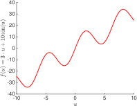
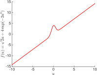
Figure 2: Plot of the link functions $f_{1}(u)=3u+10\cdot\sin(u)$ and $f_{2}(u)=\sqrt{2}u+4\exp(-2u^{2})$.

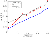
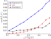
Figure 3: Cosine distances between the true parameter and the estimated parameter in the sparse SIM with the link function in (2.1) set to one of $f_{1}$ and $f_{2}$. Here we set $d=2000$. $s^{*}=5$ and vary $n$.

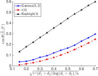
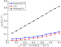
Figure 4: Cosine distances between the true parameter and the estimated parameter in the low-rank SIM for with link function in (2.1) set to one of $f_{1}$ and $f_{2}$. Here we set $d_{1}=d_{2}=20$. $r^{*}=3$ and vary $n$.

Second-order SIM: We now concentrate on the problem of sparse phase retrieval using the SDP based estimators proposed based on second-order Stein’s identity. Recall that in this case, the link function is known and existing convex and non-convex based estimators are applicable predominantly for the case of Gaussian or light-tailed data. The question of de-randomization or what are the necessary assumptions on the measurement vectors for (sparse) phase retrieval to work is an intriguing one (Gross et al., 2015). Here we demonstrate that using the proposed score-based estimators, one could deal with heavy-tailed and skewed measurement as well, which significantly extend the class of measurement vectors applicable for sparse phase retrieval.

Recall that the covariate $X$ has i.i.d. entries with distribution $p_{0}$. We set $p_{0}$ to be one of Gamma distribution with shape parameter $5$ and scale parameter $1$ and Rayleigh distribution with scale parameter $2$. The random noise $\epsilon$ is set to be standard Gaussian. Moreover, we solve the optimization problems in (4.1) and (4.2) via the alternating direction method of multipliers (ADMM) algorithm proposed in Vu et al. (2013), which introduces a dual variable to encode the constrains and updates the primal and dual variables iteratively.

We set the link function to be one of $f_{3}(u)=u^{2}$, $f_{4}=|u|$, and $f_{5}(u)=4u^{2}+3\cos(u)$. Here $f_{3}$ corresponds to the phase retrieval model and $f_{4}$ and $f_{5}$ can be viewed as its robust extension. Throughout the experiment we fix $d=500$, $s^{*}=5$ and vary $n$. The support of $\beta^{*}$ is chosen uniformly random among all subsets of $\{1,\ldots,d\}$with cardinality $s^{*}$. For each $j\in\mathop{\text{supp}}(\beta^{*})$, we set $\beta^{*}_{j}=1/\sqrt{s^{*}}\cdot\gamma_{j}$, where $\gamma_{j}$’s are i.i.d. Rademacher random variables. Furthermore, we fix the regularization parameter $\lambda=4\sqrt{\log d/n}$ and threshold parameter $\tau=20$. In addition, we adopt the cosine distance $\cos\theta(\widehat{\beta},\beta^{*})=1-|\langle\widehat{\beta},\beta^{*}\rangle|$, to measure the estimation error. We plot the cosine distance against the statistical rate of convergence $s^{*}\sqrt{\log d/n}$ in Figure 5-(a)-(c) for each link function, respectively. The plot is based on $100$ independent trials for each $n$, which shows that the estimation error is bounded by a linear function of $s^{*}\sqrt{\log d/n}$, which corroborate the theory.

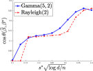
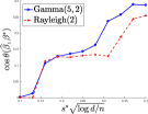
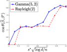
$f_{3}(u)=u^{2}$	$f_{4}(u)=|u|$,	$f_{5}(u)=4u^{2}+3\cos(u)$

Figure 5: Cosine distances between the true parameter $\beta^{*}$ and the estimated parameter $\widehat{\beta}$ in the sparse SIM with the link function being one of $f_{3}$, $f_{4}$, and $f_{5}$. Here we set $d=500$. $s^{*}=5$ and vary $n$.

6 Conclusion

In this work, we consider estimating the parametric components of single and multiple index models in the high-dimensional setting, under fairly general assumptions on the link function $f$ and response $Y$. Furthermore, our estimators are applicable in the non-Gaussian setting where $X$ is not required to satisfy restrictive Gaussian or elliptical symmetry assumptions. Our estimators are based on a data-driven truncation argument in combination with first and second-order Stein’s identity. Furthermore, we show that proposed estimators are near-optimal for several different settings.

Recently in the low-dimensional setting, for 2-layer neural networks Janzamin et al. (2015) proposed a tensor-based method for estimating the parametric components. Their estimators are sub-optimal even when we consider the low-dimensional Gaussian setting. An immediate application of our truncation based estimators enables us to obtain optimal results for a fairly general class of covariates in the low-dimensional setting. Obtaining similar optimal or near-optimal results in the high-dimensional setting is of great interest for 2-layer neural networks, albeit challenging. We plan to extend the result of this paper for 2-layer neural networks in the high-dimensional setting and report our results in the near future.

Appendix A Proofs of the Main Results

In this section, we lay out the proofs of the theorems in §3 and §4, which establish the statistical rates of convergence of our estimators.

A.1 Proof of Theorem 3.2

Proof.

Since $\widehat{\beta}$ is the solution of the optimization problem in (3.3), the first-order optimality condition states that

$$\nabla L(\widehat{\beta})+\lambda\xi=0,~{}~{}\text{where}~{}~{}\xi\in\partial\|\widehat{\beta}\|_{1}.$$ (A.1)

Then the entries of $\xi\in\mathbb{R}^{d}$ are given by

$$\xi_{j}=\mathop{\text{sign}}(\widehat{\beta}_{j}),~{}~{}\forall j\in\mathop{\text{supp}}(\widehat{\beta});$$

$$\xi_{j}\in[-1,1],~{}~{}\forall j\notin\mathop{\text{supp}}(\widehat{\beta}).$$

For any index set $\mathcal{A}\subseteq[d]$ and $z\in\mathbb{R}^{d}$, we define the restriction of $z$ to $\mathcal{A}$, $z_{\mathcal{A}}\in\mathbb{R}^{d}$, by letting

$$[z_{\mathcal{A}}]_{j}=z_{j}~{}~{}\text{if}~{}~{}j\in\mathcal{A},~{}~{}[z_{\mathcal{A}}]_{j}=0~{}~{}\text{otherwise}.$$

Here $[z_{\mathcal{A}}]_{j}$ is the $j$-th entry of $z_{\mathcal{A}}$. Let ${\mathcal{S}}=\mathop{\text{supp}}(\beta^{*})$, then we can write $\xi=\xi_{{\mathcal{S}}}+\xi_{{\mathcal{S}}^{c}}$. For notational simplicity, in the sequel, we define $\theta=\widehat{\beta}-\mu\cdot\beta^{*}$. Thus by (A.1) it holds that

$$\langle\nabla L(\widehat{\beta})-\nabla L(\mu\beta^{*}),\theta\rangle=\langle-\lambda\cdot\xi-\nabla L(\mu\beta^{*}),\theta\rangle$$

$$\qquad\leq\langle-\lambda\cdot\xi_{{\mathcal{S}}}-\lambda\cdot\xi_{{\mathcal{S}}^{c}},\theta\rangle+\|\nabla L(\mu\beta^{*})\|_{\infty}\cdot\|\theta\|_{1}.$$ (A.2)

By the definition of $\xi$, we have

$$\langle-\lambda\cdot\xi_{{\mathcal{S}}^{c}},\widehat{\beta}-\mu\beta^{*}\rangle=-\lambda\cdot\|\widehat{\beta}_{{\mathcal{S}}^{c}}\|_{1}.$$ (A.3)

Moreover, since $\|\xi\|_{\infty}\leq 1$, Hölder’s inequality implies that

$$\langle-\lambda\cdot\xi_{{\mathcal{S}}},\theta\rangle\leq\lambda\cdot\|\theta_{{\mathcal{S}}}\|_{1}.$$ (A.4)

Note that $\nabla^{2}L(\beta)=2I_{d}$. Combining (A.2), (A.3), and (A.4), we obtain

$$2\|\theta\|_{2}^{2} =\langle\nabla L(\widehat{\beta})-\nabla L(\mu\beta^{*}),\theta\rangle$$ (A.5)

$$\leq-\lambda\|\theta_{{\mathcal{S}}^{c}}\|_{1}+\lambda\|\theta_{{\mathcal{S}}}\|_{1}+\|\nabla L(\mu\beta^{*})\|_{\infty}\cdot\|\theta\|_{1}.$$ (A.6)

For an upper bound of the right-hand side of (A.5), we apply the following lemma to obtain an upper bound on $\|\nabla L(\mu\beta^{*})\|_{\infty}$.

Lemma 1 (Bound on $\|\nabla L(\mu\beta^{*})\|_{\infty}$).

We set the truncation level in (3.5) as $\tau=2(M\cdot n/\log d)^{1/4}$. Then we have

$$\mathbb{P}\Bigl{[}\|\nabla L(\mu\beta^{*})\|_{\infty}>7\sqrt{M\cdot\log d/n}\Bigr{]}\leq d^{-2}.$$

Proof.

See §B.1 for a detailed proof. ∎

Thus by Lemma 1 and the choice of $\lambda$, we have $\lambda>2\|\nabla L(\mu\beta^{*})\|_{\infty}$ with probability at least $1-d^{-2}$. This implies that

$$2\|\theta\|_{2}^{2}\leq-\lambda/2\cdot\|\theta_{{\mathcal{S}}^{c}}\|_{1}+3\lambda/2\cdot\|\theta_{{\mathcal{S}}}\|_{1}\leq 2\lambda\cdot\|\theta_{{\mathcal{S}}}\|_{1}.$$ (A.7)

Since the leftmost term in (A.7) is nonnegative, we obtain $\|\theta_{{\mathcal{S}}^{c}}\|_{1}\leq 3\cdot\|\theta_{{\mathcal{S}}}\|_{1}$. In addition, since $|{\mathcal{S}}|=s^{*}$, $\|\theta_{{\mathcal{S}}}\|_{1}\leq\sqrt{s^{*}}\cdot\|\theta_{{\mathcal{S}}}\|_{2}$. Thus by (A.7) we have $\|\theta\|_{2}\leq\sqrt{s^{*}}\cdot\lambda$. Moreover, we also have $\|\theta_{{\mathcal{S}}}\|_{1}\leq s^{*}\lambda$, which further implies that

$$\|\theta\|_{1}=\|\theta_{{\mathcal{S}}}\|_{1}+\|\theta_{{\mathcal{S}}^{c}}\|_{1}\leq 4\cdot\|\theta_{{\mathcal{S}}}\|_{1}\leq 4s^{*}\lambda.$$

Therefore, we conclude the proof. ∎

A.2 Proof of Theorem 3.3

Proof.

The proof of Theorem 3.3 is parallel to that of Theorem 3.2. Here the difference is to handle the nuclear norm regularization, instead of the $\ell_{1}$-penalty. Since $\widehat{\beta}$ is the solution of the optimization problem in (3.3), the first order optimality condition states that

$$L(\widehat{\beta})+\lambda\|\widehat{\beta}\|_{\mathop{\star}}\leq L(\mu\beta^{*})+\lambda\|\mu\beta^{*}\|_{\mathop{\star}}.$$ (A.8)

To simplify the notation, we define $\Theta=\widehat{\beta}-\mu\cdot\beta^{*}$. Since $L$ is quadratic,

$$L(\widehat{\beta})-L(\mu\beta^{*})=\langle\nabla L(\mu\beta^{*}),\Theta\rangle+2\|\Theta\|_{\mathop{\text{fro}}}^{2},$$ (A.9)

where $\nabla L$ takes values in $\mathbb{R}^{d_{1}\times d_{2}}$. Then combining (A.8), (A.9), and Hölder’s inequality, we have

$$2\|\Theta\|_{\mathop{\text{fro}}}^{2} \leq-\langle\nabla L(\mu\beta^{*}),\Theta\rangle+\lambda\|\mu\beta^{*}\|_{\mathop{\star}}-\lambda\|\widehat{\beta}\|_{\mathop{\star}}$$

$$\leq\bigl{\|}\nabla L(\mu\beta^{*})\bigr{\|}_{\mathop{\text{op}}}\cdot\|\Theta\|_{\mathop{\star}}+\lambda\|\mu\beta^{*}\|_{\mathop{\star}}-\lambda\|\widehat{\beta}\|_{\mathop{\star}}.$$ (A.10)

In the following, we focus on the term $\|\mu\beta^{*}\|_{\mathop{\star}}-\|\widehat{\beta}\|_{\mathop{\star}}$ in (A.2). Let $U\Lambda^{*}V^{\top}$ be the singular value decomposition of $\mu\beta^{*}$, where $U\in\mathbb{R}^{d_{1}\times d_{1}}$ and $V\in\mathbb{R}^{d_{2}\times d_{2}}$ are orthogonal matrices, and $\Lambda^{*}\in\mathbb{R}^{d_{1}\times d_{2}}$ be formed by the singular values of $\mu\beta^{*}$. Moreover, since $\mathrm{rank}(\beta^{*})=r^{*}$, $\Lambda^{*}$ can be written in block form as

$$\Lambda^{*}=\begin{bmatrix}\Lambda^{*}_{11}&0\\ 0&0\end{bmatrix},$$ (A.11)

where $\Lambda^{*}_{11}\in\mathbb{R}^{r^{*}\times r^{*}}$ is a diagonal matrix whose diagonal elements are the nonzero singular values of $\mu\beta^{*}$. We define $\Gamma=U^{\top}\Theta V$, which can be written in block form as

$$\Gamma=\begin{bmatrix}\Gamma_{11}&\Gamma_{12}\\ \Gamma_{21}&\Gamma_{22}\end{bmatrix},$$

where $\Gamma_{11}\in\mathbb{R}^{r^{*}\times r^{*}}$. In addition, we define matrices

$$\Gamma^{(1)}=\begin{bmatrix}0&0\\ 0&\Gamma_{22}\end{bmatrix}~{}~{}\text{and}~{}~{}\Gamma^{(2)}=\begin{bmatrix}\Gamma_{11}&\Gamma_{12}\\ \Gamma_{21}&0\end{bmatrix}.$$

Then by (A.11) and triangle inequality of the nuclear norm, we have

$$\|\widehat{\beta}\|_{\mathop{\star}}=\|\mu\beta^{*}+\Theta\|_{\mathop{\star}}=\|U(\Lambda^{*}+\Gamma)V^{\top}\|_{\mathop{\star}}$$

$$\qquad=\|\Lambda^{*}+\Gamma\|_{\mathop{\star}}\geq\|\Lambda^{*}+\Gamma^{(1)}\|_{\mathop{\star}}-\|\Gamma^{(2)}\|_{\mathop{\star}}$$

$$\qquad=\|\Lambda^{*}\|_{\mathop{\star}}+\|\Gamma^{(1)}\|_{\mathop{\star}}-\|\Gamma^{(2)}\|_{\mathop{\star}},$$ (A.12)

where the last equality follows from the fact that $\Lambda^{*}+\Gamma^{(1)}$ is block diagonal. Since $\|\mu\beta^{*}\|_{\mathop{\star}}=\|\Lambda^{*}\|_{\mathop{\star}}$, by (A.2) we obtain

$$\|\mu\beta^{*}\|_{\mathop{\star}}-\|\widehat{\beta}\|_{\mathop{\star}}\leq\|\Gamma^{(2)}\|_{\mathop{\star}}-\|\Gamma^{(1)}\|_{\mathop{\star}}.$$ (A.13)

In addition, triangle inequality implies that

$$\|\Theta\|_{\mathop{\star}}=\|U\Gamma V^{\top}\|_{\mathop{\star}}\leq\|\Gamma^{(1)}\|_{\mathop{\star}}+\|\Gamma^{(2)}\|_{\mathop{\star}}.$$ (A.14)

Thus combining (A.2), (A.13), (A.14), we have

$$2\|\Theta\|_{\mathop{\text{fro}}}^{2} \leq\bigl{(}\bigl{\|}\nabla L(\mu\beta^{*})\bigr{\|}_{\mathop{\text{op}}}+\lambda\bigr{)}\cdot\|\Gamma^{(2)}\|_{\mathop{\star}}$$

$$\qquad+\bigl{(}\bigl{\|}\nabla L(\mu\beta^{*})\bigr{\|}_{\mathop{\text{op}}}-\lambda\bigr{)}\cdot\|\Gamma^{(1)}\|_{\mathop{\star}}.$$ (A.15)

We utilize the following lemma to obtain an upper bound of $\|\nabla L(\mu\beta^{*})\|_{\mathop{\text{op}}}$.

Lemma 2 (Upper bound of $\|\nabla L(\mu\beta^{*})\|_{\mathop{\text{op}}}$).

Let $L\colon\mathbb{R}^{d_{1}\times d_{2}}\rightarrow\mathbb{R}$ be the loss function defined in (3.4) for the matrix setting. Setting

$$\kappa=2\sqrt{n\cdot\log(d_{1}+d_{2})}/\sqrt{(d_{1}+d_{2})M},$$

then it holds that

$$\mathbb{P}\Bigl{[}\|\nabla L(\mu\beta^{*})\|_{\mathop{\text{op}}}>6\sqrt{(d_{1}+d_{2})/n}\Bigr{]}\leq(d_{1}+d_{2})^{-2}.$$

Proof.

See §B.2 for a detailed proof. ∎

By Lemma 2 and the choice of $\lambda$, we conclude that $\lambda>2\cdot\|\nabla L(\mu\beta^{*})\|_{\mathop{\text{op}}}$ with probability at least $1-(d_{1}+d_{2})^{-2}$. Thus by (A.2) we have

$$2\|\Theta\|_{\mathop{\text{fro}}}^{2}\leq 3\lambda/2\cdot\|\Gamma^{(2)}\|_{\mathop{\star}}-\lambda/2\cdot\|\Gamma^{(1)}\|_{\mathop{\star}}$$ (A.16)

which implies that $\|\Gamma^{(1)}\|_{\mathop{\star}}\leq 3\cdot\|\Gamma^{(2)}\|_{\mathop{\star}}$. Moreover, by the subadditivity of rank, we obtain

$$\mathrm{rank}(\Gamma^{(2)}) \leq\mathrm{rank}\biggl{(}\begin{bmatrix}\Gamma_{11}/2&\Gamma_{12}\\ 0&0\end{bmatrix}\biggr{)}$$

$$\qquad+\mathrm{rank}\biggl{(}\begin{bmatrix}\Gamma_{11}/2&0\\ \Gamma_{21}&0\end{bmatrix}\biggr{)}=2r^{*},$$

which implies that $\|\Gamma^{(2)}\|_{\mathop{\star}}\leq\sqrt{2r^{*}}\cdot\|\Gamma^{(2)}\|_{\mathop{\text{fro}}}$ Then by (A.16) we obtain that $\|\Theta\|_{\mathop{\text{fro}}}\leq 3/\sqrt{2}\cdot\sqrt{r^{*}}\cdot\lambda$. Finally, by triangle inequality for the nuclear norm,

$$\|\Theta\|_{\mathop{\star}} =\|\Gamma\|_{\mathop{\star}}\leq\|\Gamma^{(1)}\|_{\mathop{\star}}+\|\Gamma^{(2)}\|_{\mathop{\star}}$$

$$\leq 4\cdot\|\Gamma^{(2)}\|_{\mathop{\star}}\leq 4\sqrt{2r^{*}}\|\Gamma^{(2)}\|_{\mathop{\text{fro}}}=12r^{*}\lambda.$$

Thus we conclude the proof of Theorem 3.3. ∎

A.3 Proof of Theorem 4.2

Proof.

We denote by $\widehat{W}$ the solution of the optimization problem in (4.1). In addition, we let $W^{*}=\beta^{*}{\beta^{*}}^{\top}$. In the following, we establish an upper bound for $\|\widehat{W}-W^{*}\|_{\mathop{\text{op}}}$.

Since $W^{*}$ is feasible for the optimization problem in (4.1), we have

$$\langle\widehat{W},\widetilde{\Sigma}\rangle-\lambda\|\widehat{W}\|_{1}\geq\langle W^{*},\widetilde{\Sigma}\rangle-\lambda\|W^{*}\|_{1}.$$ (A.17)

We denote $\Sigma^{*}=\mathbb{E}[Y\cdot T(X)]$. Note that $\beta^{*}$ is the leading eigenvector of $\Sigma^{*}$. Then (A.17) is equivalent to

$$\langle\widehat{W}-W^{*},\widetilde{\Sigma}-\Sigma^{*}\rangle-\lambda\|\widehat{W}\|_{1}+\lambda\|W^{*}\|_{1}$$

$$\qquad\geq\langle\Sigma^{*},W^{*}-\widehat{W}\rangle.$$ (A.18)

The following Lemma in Vu et al. (2013) (Lemma 3.1) establishes an upper bound for the first term on the left-hand side of (A.3).

Lemma 3.

Let $\Omega\in\mathbb{R}^{d\times d}$ be a symmetric matrix and let $\lambda_{1}\geq\lambda_{2}\geq\ldots\lambda_{d}$ be the eigenvalues of $\Omega$ in the descending order. For any $\ell\in[d-1]$ such that $\lambda_{\ell}-\lambda_{\ell+1}>0$, let $\Pi_{\ell}\in\mathbb{R}^{d\times d}$ be the projection matrix for the subspace spanned by the eigenvectors of $\Omega$ corresponding to $\lambda_{1},\ldots,\lambda_{\ell}$. Then for any $\Lambda\in\mathbb{R}^{d\times d}$ satisfying $0\preceq\Lambda\preceq I_{d}$ and ${\textsc{trace}}(\Lambda)=\ell$, we have

$$(\lambda_{\ell}-\lambda_{\ell+1})\cdot\|\Pi_{k}-\Lambda\|_{\mathop{\text{fro}}}^{2}\leq 2\langle\Omega,\Pi_{\ell}-\Lambda\rangle.$$

Note that $W^{*}$ is the projection matrix for the subspace spanned by $\beta^{*}$. Applying Lemma 3 to $\Sigma^{*}$ with $\ell=1$, we have

$$\langle\Sigma^{*},W^{*}-\widehat{W}\rangle\geq C_{0}/2\cdot\|\widehat{W}-W^{*}\|_{\mathop{\text{fro}}}^{2},$$ (A.19)

where $C_{0}>0$ is defined in (4.2). In addition, by Hölder’s inequality, we have

$$\langle\widehat{W}-W^{*},\widetilde{\Sigma}-\Sigma^{*}\rangle$$

$$\qquad\leq\|\widetilde{\Sigma}-\Sigma^{*}\|_{\infty}\cdot\|\widehat{W}-W^{*}\|_{1}.$$ (A.20)

In what follows, we bound $\|\widetilde{\Sigma}-\Sigma^{*}\|_{\infty}$.

Lemma 4.

Let $\widetilde{\Sigma}$ be defined in (4.5) and we define $\Sigma^{*}=\mathbb{E}[Y\cdot T(X)]$. Under Assumption 4.1, for any truncation level $\tau>0$ in (4.4), with probablity at least $1-d^{-2}$, we have

$$\|\widetilde{\Sigma}-\Sigma^{*}\|_{\infty}\leq 9M\cdot\tau^{-3}$$

$$\qquad\qquad+2\tau^{3}\cdot\log d/n+2\sqrt{5M\cdot\log d/n}.$$ (A.21)

Proof.

See §B.3 for a detailed proof. ∎

By this lemma, if we set $\tau=(1.5Mn/\log d)^{1/6}$, then with probability at least $1-d^{-2}$,

$$\|\widetilde{\Sigma}-\Sigma^{*}\|_{\infty} \leq(2\sqrt{5}+2\sqrt{6})\cdot\sqrt{M\log d/n}$$ (A.22)

$$\leq 10\sqrt{M\log d/n}.$$ (A.23)

Thus by setting $\lambda=10\sqrt{M\log d/n}$ we have $\|\widetilde{\Sigma}-\Sigma^{*}\|_{\infty}\leq\lambda$ with probability at least $1-d^{-2}$.

Then combining (A.3), (A.19), and (A.3) we have

$$\lambda\left(\|\widehat{W}-W^{*}\|_{1}-\|\widehat{W}\|_{1}+\|W^{*}\|_{1}\right)$$

$$\geq C_{0}/2\cdot\|\widehat{W}-W^{*}\|_{\mathop{\text{fro}}}^{2}.$$ (A.24)

Note that $W^{*}=\beta^{*}{\beta^{*}}^{\top}$ and that $\beta^{*}$ is $s^{*}$-sparse. We denote the support of $W^{*}$ by $\mathcal{J}$, which is given by

$$\mathcal{J}=\left\{(j,k)\in[d]\times[d]\colon\beta_{j}^{*}\cdot\beta_{k}^{*}\neq 0\right\}.$$

Then by separation of the $\ell_{1}$-norm, we have

$$\|\widehat{W}\|_{1} =\|\widehat{W}_{\mathcal{J}}\|_{1}+\|\widehat{W}_{\mathcal{J}^{c}}\|_{1}$$

$$\|\widehat{W}-W^{*}\|_{1} =\|\widehat{W}_{\mathcal{J}}-W^{*}_{\mathcal{J}}\|_{1}+\|\widehat{W}_{\mathcal{J}^{c}}\|_{1},$$

which implies that

$$\|\widehat{W}-W^{*}\|_{1}-\|\widehat{W}\|_{1}+\|W^{*}\|_{1}$$

$$\qquad=\|\widehat{W}_{\mathcal{J}}-W^{*}_{\mathcal{J}}\|_{1}-\|\widehat{W}_{\mathcal{J}}\|_{1}+\|W^{*}_{\mathcal{J}}\|_{1}$$

$$\qquad\leq 2\|\widehat{W}_{\mathcal{J}}-W^{*}_{\mathcal{J}}\|_{1}\leq 2{s^{*}}^{2}\|\widehat{W}-W^{*}\|_{\mathop{\text{fro}}}.$$ (A.25)

Here the last inequality in (A.3) follows from the fact that $|\mathcal{J}|={s^{*}}^{2}.$ Combining (A.3) and (A.3), we obtain

$$\|\widehat{W}-W^{*}\|_{\mathop{\text{fro}}}\leq 4/C_{0}\cdot s^{*}\lambda.$$ (A.26)

Since $\widehat{\beta}$ is the leading eigenvector of $\widehat{W}$, we have $\|\widehat{\beta}-\beta^{*}\|_{2}\leq\sqrt{2}\|\widehat{W}-W^{*}\|_{\mathop{\text{fro}}}\leq 4\sqrt{2}/C_{0}\cdot s^{*}\lambda$, which concludes the proof. ∎

A.4 Proof of Theorem 4.3

Proof.

The proof is similar to that of Theorem 4.2. In the case of sparse MIM, we denote $W^{*}=B^{*}{B^{*}}^{\top}$. Note that $\widehat{W}$ is the solution to the optimization problem in (4.2) and that $\widehat{B}$ consists of the top-$k$ eigenvectors of $\widehat{W}$. Then by Corollary 3.2 in Vu et al. (2013), we have

$$\inf_{O\in\mathbb{O}_{k}}\|\widehat{B}-B^{*}O\|_{\mathop{\text{fro}}}\leq\sqrt{2}\|\widehat{W}-W^{*}\|_{\mathop{\text{fro}}}.$$ (A.27)

In what follows, we derive an upper bound for $\widehat{W}-W^{*}$. Note that since $B^{*}$ is orthonormal, ${\textsc{trace}}(W^{*})=k$. Thus $W^{*}$ is feasible for (4.2), which implies

$$\langle\widehat{W}-W^{*},\widetilde{\Sigma}-\Sigma^{*}\rangle-\lambda\|\widehat{W}\|_{1}+\lambda\|W^{*}\|_{1}\geq$$

$$\langle\Sigma^{*},W^{*}-\widehat{W}\rangle.$$ (A.28)

Here we define $\Sigma^{*}=\mathbb{E}[Y\cdot T(X)]$. Note that $W^{*}$ is the projection matrix for the subspace spanned by the top-$k$ leading eigenvectors of $\Sigma^{*}$. By Lemma 3 with $\ell=k$, we have

$$\langle\Sigma^{*},W^{*}-\widehat{W}\rangle\geq\rho_{0}/2\cdot\|\widehat{W}-W^{*}\|_{\mathop{\text{fro}}}^{2},$$

where $\rho_{0}$ is the smallest eigenvalue of $\mathbb{E}[\nabla^{2}f(XB^{*})]$. Similar to the proof of Theorem 4.2, by Hölder’s inequality and (A.4), we have

$$\| \widetilde{\Sigma}-\Sigma^{*}\|_{\infty}\cdot\|\widehat{W}-W^{*}\|_{1}-\lambda\|\widehat{W}\|_{1}+\lambda\|W^{*}\|_{1}$$

$$\qquad\geq\rho_{0}/2\cdot\|\widehat{W}-W^{*}\|_{\mathop{\text{fro}}}^{2}.$$ (A.29)

By Lemma 4, if we set $\lambda=10\sqrt{M\log d/n}$, with probability at least $1-d^{-2}$, we have

$$\|\widehat{\Sigma}-\Sigma^{*}\|_{\infty}\leq\lambda.$$ (A.30)

Note that the support of $W^{*}$ is

$$\mathcal{J}\subseteq\left\{(j,k)\in[d]\times[d]\colon\|B_{j\cdot}^{*}\|_{2}\cdot\|B_{k\cdot}^{*}\|_{2}\neq 0\right\}.$$

Since $B^{*}$ is $s^{*}$-row sparse, $|\mathcal{J}|\leq{s^{*}}^{2}$. Thus (A.3) also hold for the MIM. Combining (A.4), (A.30), and (A.3), we obtain

$$\|\widehat{W}-W^{*}\|_{\mathop{\text{fro}}}\leq 4/\rho_{0}\cdot s^{*}\lambda.$$ (A.31)

Finally, combining (A.27) and (A.31), we conclude the proof. ∎

Appendix B Proof of Auxiliary Results

B.1 Proof of Lemma 1

Proof.

By definition of the loss function $L$ in (3.3), we have

$$\nabla L(\mu\beta^{*}) =2\mu\beta^{*}-\frac{2}{n}\sum_{i=1}^{n}\widetilde{Y}_{i}\cdot\widetilde{S}(X_{i})$$

$$=\mathbb{E}\bigl{[}2Y_{i}\cdot S(X_{i})\bigr{]}-\frac{2}{n}\sum_{i=1}^{n}\widetilde{Y}_{i}\cdot\widetilde{S}(X_{i}).$$

By triangle inequality,

$$\|\nabla L(\mu\beta^{*})\|_{\infty} \leq\Bigl{\|}\mathbb{E}\bigl{[}2Y\cdot S(X)\bigr{]}-\mathbb{E}\bigl{[}2\widetilde{Y}\cdot\widetilde{S}(X)\bigr{]}\Bigr{\|}_{\infty}$$

$$\qquad+\biggl{\|}\mathbb{E}\bigl{[}2\widetilde{Y}\cdot\widetilde{S}(X)\bigr{]}-\frac{2}{n}\sum_{i=1}^{n}\widetilde{Y}_{i}\cdot\widetilde{S}(X_{i})\biggr{\|}_{\infty}.$$ (B.1)

For any $j\in[d]$, by the definition of the truncated response $\widetilde{Y}$ and truncated score $\widetilde{S}$, we obtain

$$\bigl{|}\mathbb{E}\bigl{[}\widetilde{Y}\cdot\widetilde{S}_{j}(X)\bigr{]}-\mathbb{E}\bigl{[}Y\cdot S_{j}(X)\bigr{]}\bigr{|}$$

$$\leq\Bigl{|}\mathbb{E}\Bigl{\{}\widetilde{Y}\cdot\bigl{[}\widetilde{S}_{j}(X)-S_{j}(X)\bigl{]}\Bigr{\}}\Bigr{|}+\bigl{|}\mathbb{E}\bigl{[}(\widetilde{Y}-Y)\cdot S_{j}(X)\bigl{]}\bigr{|}$$

$$=\underbrace{\bigl{|}\mathbb{E}\bigl{[}\widetilde{Y}\cdot S_{j}(X)\cdot\operatorname{\mathds{1}}\{|S_{j}(X)|>\tau\}\bigr{]}\bigr{|}}_{a_{1}}$$

$$\qquad+\underbrace{\bigl{|}\mathbb{E}\bigl{[}Y\cdot S_{j}(X)\cdot\operatorname{\mathds{1}}\{|Y|>\tau\}\bigr{]}\bigr{|}}_{a_{2}}.$$ (B.2)

By Cauchy-Schwarz inequality, we have

$$a_{1}^{2} \leq\mathbb{E}\bigl{[}\widetilde{Y}^{2}S_{j}^{2}(X)\bigr{]}\cdot\mathbb{P}\bigl{[}|S_{j}(X)|\geq\tau\bigr{]}$$

$$\leq\sqrt{\mathbb{E}(\widetilde{Y}^{4})\cdot\mathbb{E}\bigl{[}S_{j}^{4}(X)\bigr{]}}\cdot\mathbb{E}\bigl{[}S_{j}^{4}(X)\bigr{]}\cdot\tau^{-4}$$

$$=M^{2}\cdot\tau^{-4},$$ (B.3)

where the second inequality follows from Chebyshev’s inequality. Similarly, for $a_{2}$ we have

$$a_{2}^{2} \leq\mathbb{E}\bigl{[}Y^{2}S_{j}^{2}(X)\bigr{]}\cdot\mathbb{P}\bigl{(}|Y|\geq\tau\bigr{)}$$

$$\leq\sqrt{\mathbb{E}(\widetilde{Y}^{4})\cdot\mathbb{E}\bigl{[}S_{j}^{4}(X)\bigr{]}}\cdot\mathbb{E}(Y^{4})\cdot\tau^{-4}$$

$$\leq M^{2}\cdot\tau^{-4}.$$ (B.4)

Thus combining (B.1), (B.1), and (B.1), we conclude that

$$\Bigl{|}\mathbb{E}\bigl{[}\widetilde{Y}\cdot\widetilde{S}_{j}(X)\bigr{]}-\mathbb{E}\bigl{[}Y\cdot S_{j}(X)\bigr{]}\Bigr{|}\leq a_{1}+a_{2}\leq 2M\cdot\tau^{-2}$$

for all $j\in[d]$. Thus choosing $\tau=2(M\cdot n/\log d)^{1/4}$, we have

$$\Bigl{\|}\mathbb{E}\bigl{[}\widetilde{Y}\cdot\widetilde{S}_{j}(X)\bigr{]}-\mathbb{E}\bigl{[}Y\cdot S_{j}(X)\bigr{]}\Bigr{\|}_{\infty}$$

$$\qquad\leq 1/2\cdot\sqrt{M\cdot\log d/n}.$$ (B.5)

Furthermore, under Assumption 4.1, the variance of $\widetilde{Y}\cdot\cdot\widetilde{S}_{j}(X)$ is bounded by

$$\operatorname{{\rm Var}}[\widetilde{Y}\cdot\widetilde{S}_{j}(X)] \leq\mathbb{E}[\widetilde{Y}^{2}\cdot\widetilde{S}_{j}^{2}(X)]$$

$$\leq\mathbb{E}[Y^{2}\cdot S_{j}^{2}(X)]$$

$$\leq\sqrt{\mathbb{E}(Y^{4})\cdot\mathbb{E}[S^{4}_{j}(X)]}\leq M.$$

Thus for the second term in (B.1), since $|\widetilde{Y}\cdot\widetilde{S}_{j}(X)|\leq\tau^{2}$, by the Bernstein inequality in Boucheron et al. (2013) (Theorem 2.10), for any $j\in[d]$ and any $t>0$, we have

$$\mathbb{P}\biggl{\{}\biggl{|}\frac{1}{n}\sum_{i=1}^{n}\widetilde{Y}_{i}\cdot\widetilde{S}_{j}(X_{i})-\mathbb{E}\bigl{[}\widetilde{Y}\cdot\widetilde{S}_{j}(X)\bigr{]}\biggr{|}$$

$$\qquad\qquad\geq\sqrt{\frac{2M\cdot t}{n}}+\frac{\tau^{2}\cdot t}{3n}\biggr{\}}\leq\exp(-t).$$ (B.6)

Taking union bound over $j\in[t]$ in (B.1) yields

$$\mathbb{P}\biggl{\{}\biggl{\|}\frac{1}{n}\sum_{i=1}^{n}\widetilde{Y}_{i}\cdot\widetilde{S}_{j}(X_{i})-\mathbb{E}\bigl{[}\widetilde{Y}\cdot\widetilde{S}_{j}(X)\bigr{]}\biggr{\|}_{\infty}$$ (B.7)

$$\qquad\qquad\geq\sqrt{\frac{2M\cdot t}{n}}+\frac{\tau^{2}\cdot t}{3n}\biggr{\}}\leq\exp(-t+\log d).$$

Finally, we plug in $\tau=2(M\cdot n/\log d)^{1/4}$ and set $t=3\log d$ in (B.7) to obtain that

$$\biggl{\|}\frac{1}{n}\sum_{i=1}^{n}\widetilde{Y}_{i}\cdot\widetilde{S}_{j}(X_{i})-\mathbb{E}\bigl{[}\widetilde{Y}\cdot\widetilde{S}_{j}(X)\bigr{]}\biggr{\|}_{\infty}$$

$$\qquad\qquad\leq(4+\sqrt{6})\sqrt{\frac{M\cdot\log d}{n}}$$ (B.8)

with probability at least $1-d^{-2}$. Finally, combining (B.1), (B.1), and (B.1), we conclude the proof. ∎

B.2 Proof of Lemma 2

Proof.

For loss function $L$ defined in (3.3) in the matrix setting, we have

$$\nabla L(\mu\beta^{*})=2\mu\beta^{*}-\frac{2}{\kappa\cdot n}\sum_{i=1}^{n}\psi\bigl{[}\kappa\cdot Y_{i}\cdot S(X_{i})\bigr{]}$$

$$\qquad=2\mathbb{E}[Y\cdot S(X)]-\frac{2}{\kappa\cdot n}\sum_{i=1}^{n}\psi\bigl{[}\kappa\cdot Y_{i}\cdot S(X_{i})\bigr{]}.$$ (B.9)

Here the last equality follows from the generalized Stein’s identity. In the sequel, we apply results in Minsker (2016) to bound $\|\nabla L(\mu\beta^{*})\|_{\mathop{\text{op}}}$. To begin with, we first consider the operator norm of $\mathbb{E}[Y^{2}\cdot S(X)S(X)^{\top}]\in\mathbb{R}^{d_{!}\times d_{2}}$ and $\mathbb{E}[Y^{2}\cdot S(X)^{\top}S(X)]\in\mathbb{R}^{d_{2}\times d_{2}}$. For notational simplicity, we denote by $S_{j,\cdot}(\cdot)\in\mathbb{R}^{d_{2}}$ $S_{\cdot,k}(\cdot)\in\mathbb{R}^{d_{1}}$ the $j$-th row and $k$-the column of the score function $S(\cdot)$, respectively. For any $u\in{\mathcal{S}}^{d_{1}-1}$, by Cauchy-Schwarz inequality we have

$$\mathbb{E}[Y^{2}\cdot u^{\top}S(X)S(X)^{\top}u]$$

$$\qquad=\sum_{k=1}^{d_{2}}\mathbb{E}\bigl{\{}[Y^{2}\cdot S_{\cdot,k}(X)^{\top}u]^{2}\bigr{\}}$$

$$\qquad\leq d_{2}\cdot\sqrt{\mathbb{E}(Y^{4})\cdot\mathbb{E}\bigl{\{}[S_{\cdot,1}(X)^{\top}u]^{4}\bigr{\}}},$$ (B.10)

where we use the fact that the entries of $S(X)$ are i.i.d. Since $\mathbb{E}[S_{ij}(X)]=0$ and $\mathbb{E}[S_{ij}^{4}(X)]\leq M$, by Cauchy-Schwarz inequality we obtain that

$$\mathbb{E}\bigl{\{}[S_{\cdot,1}(X)^{\top}u]^{4}\bigr{\}}$$

$$\qquad=\sum_{j_{1}=1}^{d}\sum_{j_{2}=1}^{d}\mathbb{E}[S_{j_{1},1}(X)^{2}\cdot S_{j_{2},1}^{2}(X)]\cdot u_{j_{i}}^{2}u_{j_{2}}^{2}$$

$$\qquad\leq\sum_{j_{1}=1}^{d}\sum_{j_{2}=1}^{d}\sqrt{\mathbb{E}[S_{j_{1},1}^{4}(X)]\cdot\mathbb{E}[S_{j_{2},1}^{4}(X)]}\cdot u_{j_{i}}^{2}u_{j_{2}}^{2}$$

$$\qquad\leq M\sum_{j_{1}=1}^{d}\sum_{j_{2}=1}^{d}u_{j_{i}}^{2}u_{j_{2}}^{2}=M.$$ (B.11)

Thus combining (B.2) and (B.2) we obtain that

$$\mathbb{E}[Y^{2}\cdot u^{\top}S(X)S(X)^{\top}u]\leq d_{2}\cdot M,$$

which implies that $\|\mathbb{E}[Y^{2}\cdot S(X)S(X)^{\top}]\|_{\mathop{\text{op}}}\leq d_{2}\cdot M$. Similarly, we obtain $\|\mathbb{E}[Y^{2}\cdot S(X)^{\top}S(X)]\|_{\mathop{\text{op}}}\leq d_{1}\cdot M.$ Thus by Corollary 3.1 in Minsker (2016), we have

$$\mathbb{P}\biggl{\{}\biggl{\|}\frac{1}{\kappa\cdot n}\sum_{i=1}^{n}\psi\bigl{[}\kappa\cdot Y_{i}\cdot S(X_{i})\bigr{]}-\mathbb{E}[Y\cdot S(X)]\biggr{\|}_{\mathop{\text{op}}}\geq\frac{t}{\sqrt{n}}\biggr{\}}$$

$$\qquad\leq 2(d_{1}+d_{2})\exp\bigl{[}-\kappa t\sqrt{n}+\kappa^{2}(d_{1}+d_{2})M/2\bigr{]}$$ (B.12)

for any $t>0$ and $\kappa>0$. We set

$$\kappa=2\sqrt{n\cdot\log(d_{1}+d_{2})}/\sqrt{(d_{1}+d_{2})M}$$

and $t=\sqrt{(d_{1}+d_{2})M}\cdot s$ in (B.2), which implies that

$$\mathbb{P}\biggl{\{}\biggl{\|}\frac{1}{\kappa\cdot n}\sum_{i=1}^{n}\psi\bigl{[}\kappa\cdot Y_{i}\cdot S(X_{i})\bigr{]}-\mathbb{E}[Y\cdot S(X)]\biggr{\|}_{\mathop{\text{op}}}$$

$$\qquad\qquad\geq\sqrt{\frac{(d_{1}+d_{2})M}{n}}\cdot s\biggr{\}}$$

$$\qquad\leq 2(d_{1}+d_{2})\cdot\exp\bigl{[}-2\sqrt{\log(d_{1}+d_{2})}\cdot s$$

$$\qquad\qquad+2\cdot\log(d_{1}+d_{2})\bigr{]}.$$ (B.13)

Now we set $s=3\cdot\sqrt{\log(d_{1}+d_{2})}$, which implies that the right-hand side of (B.2) is less than

$$2(d_{1}+d_{2})\cdot\exp\bigl{[}-6\log(d_{1}+d_{2})+2\cdot\log(d_{1}+d_{2})\bigr{]}$$

$$\quad\leq(d_{1}+d_{2})^{2}\cdot\exp\bigl{[}-4\cdot\log(d_{1}+d_{2})\bigr{]}=(d_{1}+d_{2})^{-2}.$$

Therefore, combining (B.2) and (B.2) we obtain that

$$\|\nabla L(\mu\beta^{*})\|_{\mathop{\text{op}}}\leq 6\sqrt{(d_{1}+d_{2})\cdot M/n}\cdot\sqrt{\log(d_{1}+d_{2})}$$

with probability at least $1-(d_{1}+d_{2})^{-2}$, which concludes the proof.

∎

B.3 Proof of Lemma 4

Proof.

By triangle inequailty, we have

$$\|\widetilde{\Sigma}-\Sigma^{*}\|_{\infty}\leq\|\widetilde{\Sigma}-\mathbb{E}\widetilde{\Sigma}\|_{\infty}+\|\mathbb{E}\widetilde{\Sigma}-\Sigma^{*}\|_{\infty}.$$ (B.14)

In the sequel, we bound the second term on the right-hand side of (B.14), which controls the bias of truncation. For each $j,k\in[d]$, we have

$$\left|\mathbb{E}\widetilde{\Sigma}_{jk}-\Sigma^{*}_{jk}\right|\leq\left|\mathbb{E}\bigl{[}\widetilde{Y}\cdot\widetilde{T}_{jk}(X)\bigr{]}-\mathbb{E}\bigl{[}Y\cdot T_{jk}(X)\bigr{]}\right|$$

$$\qquad\leq\left|\mathbb{E}\bigl{\{}\widetilde{Y}\cdot\bigl{[}\widetilde{T}_{jk}(X)-T_{jk}(X)\bigr{]}\bigr{\}}\right|$$

$$\qquad\qquad+\left|\mathbb{E}\bigl{[}(\widetilde{Y}-Y)\cdot T_{jk}(X)\bigr{]}\right|.$$ (B.15)

For the first term in (B.3), note that

$$\widetilde{T}_{jk}(X)-T_{jk}(X)=T_{jk}(X)\cdot\operatorname{\mathds{1}}\{|T_{jk}(X)|\geq\tau^{2}\}.$$

Then by Cauchy-Schwarz inequality we have

$$\left|\mathbb{E}\left\{\widetilde{Y}\cdot\left[\widetilde{T}_{jk}(X)-T_{jk}(X)\right]\right\}\right|^{2}$$

$$\qquad=\left|\mathbb{E}\left[\widetilde{Y}\cdot T_{jk}(X)\cdot\operatorname{\mathds{1}}\{|T_{jk}(X)|\geq\tau^{2}\}\right]\right|^{2}$$

$$\qquad\leq\mathbb{E}\left[\widetilde{Y}^{2}\cdot T_{jk}^{2}(X)\right]\cdot\mathbb{P}\left[|T_{jk}(X)|\geq\tau^{2}\right].$$ (B.16)

Furthermore, by Hölder’s inequality, we have

$$\mathbb{E}\left[\widetilde{Y}^{2}\cdot T_{jk}^{2}(X)\right]\leq\left[\mathbb{E}(\widetilde{Y}^{6})\right]^{1/3}\cdot\left\{\mathbb{E}\left[|T_{jk}(X)|^{3}\right]\right\}^{2/3}$$

$$\qquad\leq\left[\mathbb{E}(Y^{6})\right]^{1/3}\left\{\mathbb{E}\left[|T_{jk}^{3}(X)|\right]\right\}^{2/3}.$$ (B.17)

If $j\neq k$, by the definition of $T(x)$ in (4.1), we have $T_{jk}(x)=S_{j}(x)\cdot S_{k}(x)$, $\forall x\in\mathbb{R}^{d}$. Then by Cauchy-Schwarz inequality, we have

$$\mathbb{E}\left[|T_{jk}^{3}(X)|\right]=\mathbb{E}\left[|S_{j}(X)|^{3}\cdot|S_{k}(X)|^{3}\right]$$

$$\qquad\leq\sqrt{\mathbb{E}[S_{j}^{6}(X)]\cdot\mathbb{E}[S_{k}^{6}(X)]}=\mathbb{E}[S_{j}^{6}(X)].$$ (B.18)

In addition, if $j=k$, by (4.1), $T_{jj}(x)=S_{j}^{2}(x)-s_{1}(x_{j})$. Since $(a+b)^{3}\leq 4(a^{3}+b^{3})$ for any $a,b>0$, we have

$$\mathbb{E}\left[|T_{jj}^{3}(X)|\right]\leq 4\mathbb{E}[S_{j}^{6}(X)]+4\mathbb{E}\left[|s_{1}^{3}(X_{j})|\right].$$ (B.19)

Moreover, by (B.3), (B.3), and the Markov’s inequality that

$$\mathbb{P}\left[|T_{jk}(X)|\geq\tau^{2}\right]\leq\mathbb{E}\left[|T_{jk}^{3}(X)|\right]\cdot\tau^{-6},$$

we further have

$$\left|\mathbb{E}\bigl{\{}\widetilde{Y}\cdot\bigl{[}\widetilde{T}_{jk}(X)-T_{jk}(X)\bigr{]}\bigr{\}}\right|^{2}$$

$$\qquad\leq\left[\mathbb{E}(Y^{6})\right]^{1/3}\cdot\left\{\mathbb{E}\left[|T_{jk}^{3}(X)|\right]\right\}^{5/3}\cdot\tau^{-6}$$

$$\qquad\leq 32M^{2}\cdot\tau^{-6}.$$ (B.20)

Here the last inequality follows from combining Assumption 4.1, (B.3), and (B.19).

Similarly, for the second term in (B.3), by the Hölder’s inequality and the Markov’s inequality we obtain that

$$\left|\mathbb{E}\left[(\widetilde{Y}-Y)\cdot T_{jk}(X)\right]\right|^{2}$$

$$\qquad\leq\left[\mathbb{E}(Y^{6})\right]^{1/3}\cdot\left\{\mathbb{E}\left[|T_{jk}^{3}(X)|\right]\right\}^{2/3}\cdot\mathbb{P}(|Y|\geq\tau)$$

$$\qquad\leq\left[\mathbb{E}(Y^{6})\right]^{4/3}\cdot\left\{\mathbb{E}\left[|T_{jk}^{3}(X)|\right]\right\}^{2/3}\cdot\tau^{-6}$$

$$\qquad\leq 4M^{2}\cdot\tau^{-6}.$$ (B.21)

Thus, combining (B.3), (B.3), and (B.3), we have

$$\|\mathbb{E}\widetilde{\Sigma}-\Sigma^{*}\|_{\infty}\leq 9M\cdot\tau^{-3}.$$ (B.22)

In what follows, we give a high-probability bound on $\|\widetilde{\Sigma}-\mathbb{E}\widetilde{\Sigma}\|_{\infty}$ using concentration inequalities, which combined with B.22, concludes the proof.

For any $j,k\in[d],$ note that $|\widetilde{Y}\cdot\widetilde{T}_{jk}(X)|\leq\tau^{3}$. In addition, by assumption 4.1, its variance is bounded by

$$\operatorname{{\rm Var}}\left[\widetilde{Y}\cdot\widetilde{T}_{jk}(X)\right]\leq\mathbb{E}\left[Y^{2}\cdot T_{jk}^{2}(X)\right]$$

$$\qquad\leq\left[\mathbb{E}(Y^{6})\right]^{1/3}\cdot\left\{\mathbb{E}\left[|T_{jk}^{3}(X)|\right]\right\}^{2/3}\leq 2M.$$

Now we apply the Bernstein’s inequality (Boucheron et al., 2013) (Theorem 2.10) to $\{\widetilde{Y}_{i}\cdot\widetilde{T}_{jk}(X_{i})\}_{i\in[n]}$ and obtain that

$$\mathbb{P}\biggl{\{}\biggl{|}\frac{1}{n}\sum_{i=1}^{n}\widetilde{Y}_{i}\cdot\widetilde{T}_{jk}(X_{i})-\mathbb{E}\left[\widetilde{Y}\cdot\widetilde{T}_{jk}(X)\right]\biggr{|}$$

$$\qquad\geq\sqrt{\frac{4M\cdot t}{n}}+\frac{\tau^{3}\cdot t}{3n}\biggr{\}}\leq 2\exp(-t).$$ (B.23)

Taking a union bound over $j,k\in[d]$ in (B.3), we obtain that

$$\mathbb{P}\left[\|\widetilde{\Sigma}-\mathbb{E}\widetilde{\Sigma}\|_{\infty}\geq\sqrt{4M\cdot t/n}+\tau^{3}\cdot t/(3n)\right]$$

$$\qquad\leq 2\exp(-t+2\log d).$$ (B.24)

Choosing $t=5\log d$ in (B.3), we obtain that

$$\|\widetilde{\Sigma}-\mathbb{E}\widetilde{\Sigma}\|_{\infty}$$

$$\qquad\leq 2\sqrt{5M\log d/n}+2\tau^{3}\cdot\log d/n$$ (B.25)

holds with probability at least $1-d^{-2}$. Finally, combining (B.22) and (B.3), we complete the proof of Lemma 4. ∎

References

- Ai et al. (2014) Albert Ai, Alex Lapanowski, Yaniv Plan, and Roman Vershynin. One-bit compressed sensing with non-gaussian measurements. Linear Algebra and its Applications, 441:222–239, 2014.
- Alquier and Biau (2013) Pierre Alquier and Gérard Biau. Sparse single-index model. The Journal of Machine Learning Research, 14(1):243–280, 2013.
- Boucheron et al. (2013) Stéphane Boucheron, Gábor Lugosi, and Pascal Massart. Concentration inequalities: A nonasymptotic theory of independence. Oxford university press, 2013.
- Boufounos and Baraniuk (2008) Petros T Boufounos and Richard G Baraniuk. 1-bit compressive sensing. In Information Sciences and Systems, 2008. CISS 2008. 42nd Annual Conference on, pages 16–21. IEEE, 2008.
- Bühlmann and van de Geer (2011) Peter Bühlmann and Sara van de Geer. Statistics for high-dimensional data: methods, theory and applications. Springer Science & Business Media, 2011.
- Cai et al. (2015) T Tony Cai, Xiaodong Li, and Zongming Ma. Optimal rates of convergence for noisy sparse phase retrieval via thresholded wirtinger flow. arXiv preprint arXiv:1506.03382, 2015.
- Candès et al. (2013) Emmanuel J Candès, Thomas Strohmer, and Vladislav Voroninski. Phaselift: Exact and stable signal recovery from magnitude measurements via convex programming. Communications on Pure and Applied Mathematics, 66(8):1241–1274, 2013.
- Candes et al. (2015) Emmanuel J Candes, Xiaodong Li, and Mahdi Soltanolkotabi. Phase retrieval via wirtinger flow: Theory and algorithms. IEEE Transactions on Information Theory, 2015.
- Catoni et al. (2012) Olivier Catoni et al. Challenging the empirical mean and empirical variance: a deviation study. Annales de l’Institut Henri Poincaré, Probabilités et Statistiques, 48(4):1148–1185, 2012.
- Chen et al. (2016) Han Chen, Garvesh Raskutti, and Ming Yuan. Non-convex projected gradient descent for generalized low-rank tensor regression. arXiv preprint arXiv:1611.10349, 2016.
- Chen et al. (2010) Xin Chen, Changliang Zou, and R Dennis Cook. Coordinate-independent sparse sufficient dimension reduction and variable selection. The Annals of Statistics, 38(6):3696–3723, 2010.
- Davenport et al. (2014) Mark A Davenport, Yaniv Plan, Ewout van den Berg, and Mary Wootters. 1-bit matrix completion. Information and Inference, 3(3):189–223, 2014.
- Fan et al. (2011) J. Fan, J. Lv, and L. Qi. Sparse high-dimensional models in economics. Annual review of economics, 3(1):291–317, 2011.
- Fan et al. (2016) Jianqing Fan, Weichen Wang, and Ziwei Zhu. A shrinkage principle for heavy-tailed data: High-dimensional robust low-rank matrix recovery. arXiv preprint arXiv:1603.08315, 2016.
- Friedland and Lim (2014) Shmuel Friedland and Lek-Heng Lim. Nuclear norm of higher-order tensors. arXiv preprint arXiv:1410.6072, 2014.
- Goldstein et al. (2016) Larry Goldstein, Stanislav Minsker, and Xiaohan Wei. Structured signal recovery from non-linear and heavy-tailed measurements. arXiv preprint arXiv:1609.01025, 2016.
- Gross et al. (2015) David Gross, Felix Krahmer, and Richard Kueng. A partial derandomization of phaselift using spherical designs. Journal of Fourier Analysis and Applications, 2015.
- Horowitz (2009) Joel L Horowitz. Semiparametric and nonparametric methods in econometrics, volume 12. Springer, 2009.
- Jaganathan et al. (2015) Kishore Jaganathan, Yonina C Eldar, and Babak Hassibi. Phase retrieval: An overview of recent developments. arXiv preprint arXiv:1510.07713, 2015.
- Janzamin et al. (2014) Majid Janzamin, Hanie Sedghi, and Anima Anandkumar. Score function features for discriminative learning: Matrix and tensor framework. arXiv preprint arXiv:1412.2863, 2014.
- Janzamin et al. (2015) Majid Janzamin, Hanie Sedghi, and Anima Anandkumar. Beating the perils of non-convexity: Guaranteed training of neural networks using tensor methods. arXiv preprint arXiv:1506.08473, 2015.
- Jiang and Liu (2014) B. Jiang and J. S. Liu. Variable selection for general index models via sliced inverse regression. The Annals of Statistics, 42(5):1751–1786, 2014.
- Kakade et al. (2011) Sham M Kakade, Varun Kanade, Ohad Shamir, and Adam Kalai. Efficient learning of generalized linear and single index models with isotonic regression. In Advances in Neural Information Processing Systems, pages 927–935, 2011.
- Kalai and Sastry (2009) Adam Tauman Kalai and Ravi Sastry. The isotron algorithm: High-dimensional isotonic regression. In Conference on Learning Theory, 2009.
- Krauthgamer et al. (2015) Robert Krauthgamer, Boaz Nadler, Dan Vilenchik, et al. Do semidefinite relaxations solve sparse pca up to the information limit? The Annals of Statistics, 43(3):1300–1322, 2015.
- Lecué and Mendelson (2015) Guillaume Lecué and Shahar Mendelson. Minimax rate of convergence and the performance of empirical risk minimization in phase retrieval. Electron. J. Probab, 20(57):1–29, 2015.
- Li (1991) Ker-Chau Li. Sliced inverse regression for dimension reduction. Journal of the American Statistical Association, 86(414):316–327, 1991.
- Li (1992) Ker-Chau Li. On principal Hessian directions for data visualization and dimension reduction: Another application of Stein’s lemma. Journal of the American Statistical Association, 87(420):1025–1039, 1992.
- Li and Duan (1989) Ker-Chau Li and Naihua Duan. Regression analysis under link violation. The Annals of Statistics, 17(3):1009–1052, 1989.
- Li and Voroninski (2013) Xiaodong Li and Vladislav Voroninski. Sparse signal recovery from quadratic measurements via convex programming. SIAM Journal on Mathematical Analysis, 45(5):3019–3033, 2013.
- Lin et al. (2015) Q. Lin, Z. Zhao, and J. S. Liu. On consistency and sparsity for sliced inverse regression in high dimensions. arXiv preprint arXiv:1507.03895, 2015.
- Lin et al. (2017) Qian Lin, Xinran Li, Dongming Huang, and Jun S Liu. On the optimality of sliced inverse regression in high dimensions. arXiv preprint arXiv:1701.06009, 2017.
- Loh and Wainwright (2015) Po-Ling Loh and Martin J Wainwright. Regularized m-estimators with nonconvexity: Statistical and algorithmic theory for local optima. Journal of Machine Learning Research, 16:559–616, 2015.
- McLachlan and Peel (2004) Geoffrey McLachlan and David Peel. Finite mixture models. John Wiley & Sons, 2004.
- Mendelson (2014) Shahar Mendelson. Learning without concentration. In Proceedings of The 27th Conference on Learning Theory, pages 25–39, 2014.
- Minsker (2016) Stanislav Minsker. Sub-gaussian estimators of the mean of a random matrix with heavy-tailed entries. arXiv preprint arXiv:1605.07129, 2016.
- Mu et al. (2014) Cun Mu, Bo Huang, John Wright, and Donald Goldfarb. Square deal: Lower bounds and improved relaxations for tensor recovery. In Proceedings of The 31st International Conference on Machine Learning, pages 73–81, 2014.
- Negahban et al. (2012) Sahand N. Negahban, Pradeep Ravikumar, Martin J. Wainwright, and Bin Yu. A unified framework for high-dimensional analysis of -estimators with decomposable regularizers. Statistical Science, 27(4):538–557, 11 2012.
- Neykov et al. (2016) Matey Neykov, Zhaoran Wang, and Han Liu. Agnostic estimation for misspecified phase retrieval models. In Advances in Neural Information Processing Systems, pages 4089–4097, 2016.
- Oliveira (2013) Roberto Imbuzeiro Oliveira. The lower tail of random quadratic forms, with applications to ordinary least squares and restricted eigenvalue properties. arXiv preprint arXiv:1312.2903, 2013.
- Plan and Vershynin (2016) Yaniv Plan and Roman Vershynin. The generalized lasso with non-linear observations. IEEE Transactions on information theory, 62(3):1528–1537, 2016.
- Radchenko (2015) Peter Radchenko. High dimensional single index models. Journal of Multivariate Analysis, 139:266–282, 2015.
- Stein (1972) C. Stein. A bound for the error in the normal approximation to the distribution of a sum of dependent random variables. In Proceedings of the Sixth Berkeley Symposium on Mathematical Statistics and Probability, Volume 2: Probability Theory. The Regents of the University of California, 1972.
- Stein et al. (2004) Charles Stein, Persi Diaconis, Susan Holmes, Gesine Reinert, et al. Use of exchangeable pairs in the analysis of simulations. In Stein’s Method. Institute of Mathematical Statistics, 2004.
- Sun et al. (2016) Ju Sun, Qing Qu, and John Wright. A geometric analysis of phase retrieval. arXiv preprint arXiv:1602.06664, 2016.
- Thrampoulidis et al. (2015) Christos Thrampoulidis, Ehsan Abbasi, and Babak Hassibi. Lasso with non-linear measurements is equivalent to one with linear measurements. Advances in Neural Information Processing Systems, 2015.
- Vu et al. (2013) Vincent Q Vu, Juhee Cho, Jing Lei, and Karl Rohe. Fantope projection and selection: A near-optimal convex relaxation of sparse pca. In Advances in neural information processing systems, pages 2670–2678, 2013.
- Waldspurger et al. (2015) Irène Waldspurger, Alexandre d’Aspremont, and Stéphane Mallat. Phase recovery, maxcut and complex semidefinite programming. Mathematical Programming, 149(1-2):47–81, 2015.
- Wang et al. (2016) Tengyao Wang, Quentin Berthet, Richard J Samworth, et al. Statistical and computational trade-offs in estimation of sparse principal components. The Annals of Statistics, 44(5):1896–1930, 2016.
- Wang et al. (2014) Zhaoran Wang, Huanran Lu, and Han Liu. Tighten after relax: Minimax-optimal sparse pca in polynomial time. In Advances in neural information processing systems, pages 3383–3391, 2014.
- Yang et al. (2015) Zhuoran Yang, Zhaoran Wang, Han Liu, Yonina C Eldar, and Tong Zhang. Sparse nonlinear regression: Parameter estimation and asymptotic inference. International Conference on Machine Learning, 2015.
- Yang et al. (2017a) Zhuoran Yang, Krishnakumar Balasubramanian, and Han Liu. High-dimensional non-gaussian single index models via thresholded score function estimation. In International Conference on Machine Learning, pages 3851–3860, 2017a.
- Yang et al. (2017b) Zhuoran Yang, Krishnakumar Balasubramanian, Zhaoran Wang, and Han Liu. Estimating high-dimensional non-gaussian multiple index models via stein’s lemma. In Advances in Neural Information Processing Systems, pages 6097–6106, 2017b.
- Zhu et al. (2006) Lixing Zhu, Baiqi Miao, and Heng Peng. On sliced inverse regression with high-dimensional covariates. Journal of the American Statistical Association, 101(474):630–643, 2006.