Liouville action and Holography on quasi-Fuchsian deformation spaces

Abstract.

We study the Liouville action for quasi-Fuchsian groups with parabolic and elliptic elements. In particular, when the group is Fuchsian, the contribution of elliptic elements to the classical Liouville action is derived in terms of the Bloch-Wigner functions. We prove the first and second variation formulas for the classical Liouville action on the quasi-Fuchsian deformation space. We prove an equality expressing the holography principle, which relates the Liouville action and the renormalized volume for quasi-Fuchsian groups with parabolic and elliptic elements. We also construct the potential functions of the Kähler forms corresponding to the Takhtajan-Zograf metrics associated to the elliptic elements in the quasi-Fuchsian groups.

1. Introduction

In this paper, we study the Liouville action for quasi-Fuchsian groups with parabolic and elliptic elements. We also prove an equality expressing the holography principle, that is, a relationship between the Liouville action and the renormalized volume for quasi-Fuchsian groups. This work can be considered as a continuation of the previous papers [9], [7] where we restricted types of the quasi-Fuchsian groups. In [7], we considered the case of quasi-Fuchsian groups with only parabolic elements. A main novelty of this paper is the derivation of the contributions of the elliptic elements to the Liouville action and the holography principle. Interestingly, such new contributions are given in terms of the Bloch-Wigner functions, which are variants of the dilogarithm functions.

Now we introduce some notations to explain main results of this paper. Let $\Gamma$ be a quasi-Fuchsian group in $\text{PSL}(2,\mathbb{C})$ with its region of discontinuity $\Omega=\Omega_{1}\sqcup\Omega_{2}$. Let $X\simeq\Gamma\backslash\Omega_{1}$ and $Y\simeq\Gamma\backslash\Omega_{2}$ be the corresponding Riemann surfaces with opposite orientations. We allow $\Gamma$ to have some parabolic elements and elliptic elements, so that the Riemann surfaces $X$ and $Y$ have possibly punctures and ramification points. We also assume some topological conditions so that $X$ and $Y$ can be equipped with hyperbolic metrics. The first part of this paper deals with the Liouville action for these Riemann surfaces. Since these Riemann surfaces have punctures and ramification points, we need to check behaviours of the metrics near these points in order to define the Liouville action. By some estimates, we show that the Liouville action can be defined for the hyperbolic metric for Riemann surfaces with punctures and ramification points. The Liouville action defined for the hyperbolic metric is called classical. The new results of the first part are descriptions of the classical Liouville action over the deformation space $\mathfrak{D}(\Gamma)$ of the quasi-Fuchsian groups. For the precise definitions of these, see the subsection 2.2 and the paragraph near equality (2.3) respectively. In particular, we derive the contribution of the elliptic elements to the classical Liouville action when the group $\Gamma$ is Fuchsian and obtain the first and second variational formulas of the classical Liouville action over $\mathfrak{D}(\Gamma)$. The following theorem is given at Theorems 2.5, 3.3, and 3.5 with more explanations.

Theorem 1.1.

When $\Gamma$ is Fuchsian, the classical Liouville action $S$ is given by

$$S=8\pi\chi(X)+4\sum_{j=1}^{r}D\left(e^{\frac{2\pi i}{m_{j}}}\right).$$

Here $\chi(X)$ is given by (2.1), $D(z)$ denotes the Bloch-Wigner function given in (2.20), and $m_{j}$ denotes the ramification index for $j=1,\ldots,r$. For the classical Liouville action $S$ on the deformation space $\mathfrak{D}(\Gamma)$,

$$\partial{S}=\vartheta,\qquad\bar{\partial}\partial S=-2i\omega_{WP}.$$

Here $\vartheta$ denotes the $(1,0)$-form over $\mathfrak{D}(\Gamma)$ corresponding to the holomorphic quadratic differential $2\varphi_{zz}-\varphi_{z}^{2}$ for the hyperbolic metric $e^{\varphi(z)}|dz|^{2}$ and $\omega_{WP}$ denotes the Weil-Petersson symplectic form over $\mathfrak{D}(\Gamma)$.

Although the above results of the Liouville action hold only along the hyperbolic metrics, the Liouville action can be defined for any metrics which have same singular behaviours as the hyperbolic metric near punctures and ramifications points. We denote the set of such metrics over $X\sqcup Y$ by $\mathcal{CM}(X\sqcup Y)$. By the holography principle, the Liouville action of a metric is expected to have a relationship with the renormalized volume of a hyperbolic 3-manifold which has the given pair of Riemann surfaces $X\sqcup Y$ as conformal boundaries [5], [9], [7]. Such a hyperbolic 3-manifold $M$ is given by the quotient of the hyperbolic 3-space by the quasi-Fuchsian group $\Gamma$. Since we allow punctures and ramification points for $X$ and $Y$, correspondingly the manifold $M$ has rank one cusps and conical singularities of codimension 2. The second part of this paper deals with the proof of this relationship expected from the holography principle. The main task for this is to elaborate the analysis for contribution from rank one cusps and conical singularities. The case of rank one cusps was also discussed briefly in [7] and these singular structures did not produce any additional terms, but the conical singularities of codimension 2 produce some additional terms expressed by the Bloch-Wigner functions. A metric $e^{\phi(z)}|dz|^{2}\in\mathcal{CM}(X\sqcup Y)$ is used to renormalize the hyperbolic volume of $M$ near conformal boundaries $X\sqcup Y$ as in other works [3], [5], [9], but we also need other regularization process near rank one cusps and conical singularities of codimension 2. In this way, we can regularize the hyperbolic volume of $M$ and define the Einstein-Hilbert action $\mathcal{E}[\phi]$ by (4.12), which is the same as $-4$ times of the renormalized volume. The following theorem is given at Theorem 4.8 with more explanations.

Theorem 1.2.

For $e^{\phi(z)}|dz|^{2}\in\mathcal{CM}(X\sqcup Y)$,

$$\mathcal{E}[\phi]=S[\phi]-\iint\limits_{X\sqcup Y}e^{\phi(z)}d^{2}z-8\pi\chi(X)\log 2-4\sum_{j=1}^{r}D\left(e^{\frac{2\pi i}{m_{j}}}\right).$$

In the above equality, the terms given by the Bloch-Wigner functions are derived from the conical singularities of codimension 2 of $M$. Correspondingly, as we stated in Theorem 1.1, the exactly same terms appear as the contribution of the elliptic elements to the classical Liouville action $S$ when $\Gamma$ is Fuchsian. A hyperbolic manifold with conical singularities of codimension 2 is called a hyperbolic manifold with particles in [4]. Hence, it seems to be interesting to understand the terms given by the Bloch-Wigner functions in Theorem 1.2 from the viewpoint of [4].

Recently Takhtajan and Zograf introduced a metric associated to a ramification point over a Riemann surface in [11]. The precise definition for this is given in Section 5. For a quasi-Fuchsian group with elliptic elements, this metric can be defined for each pair of ramification points in $X\sqcup Y$ determined by an elliptic element. Considering Theorems 1.1 and 1.2, one would naturally ask about the construction of potential functions of the Kähler forms corresponding to these metrics on the quasi-Fuchsian deformation space $\mathfrak{D}(\Gamma)$. Employing machinery to prove aforementioned theorems, we construct such potential functions in two ways. The first one is constructed analytically from the hyperbolic metric over $X\sqcup Y$, and the second one is constructed geometrically from $M$. The precise definitions of these and the corresponding results are given in Section 5.

Now we explain the structure of this paper. In Section 2, we construct the Liouville action over quasi-Fuchsian deformation space $\mathfrak{D}(\Gamma)$ and derive the elliptic contribution to the classical Liouville action when $\Gamma$ is Fuchsian. In Section 3, we prove the results for variation formulas of the classical Liouville action. In Section 4, we prove the equality relating the Liouville action to the Einstein-Hilbert action. In Section 5, we construct potential functions of the Takhtajan-Zograf metric associated to elliptic elements in $\Gamma$. In Appendix A, we provide some estimates for the hyperbolic metric near punctures and ramification points.

Acknowledgements

The work of J. Park was partially supported by Samsung Science and Technology Foundation under Project Number SSTF-BA1701-02. We would like to thank L. Takhtajan and K. Krasnov for giving constructive comments to the first draft of this paper.

2. The Liouville action functional on quasi-Fuchsian deformation spaces

Consider a Riemann surface of finite type $X$, with genus $g$, $n\geq 0$ punctures, and $r\geq 0$ ramified points with ramification indices $m_{1}$, $m_{2}$, $\ldots$, $m_{r}$, where $2\leq m_{1}\leq m_{2}\leq\ldots\leq m_{r}$. We say that the Riemann surface is of type $(g,n;m_{1},m_{2},\ldots,m_{r})$. The characteristic of the surface $X$ is given by

$$\chi(X)=2g-2+n+\sum_{i=1}^{r}\left(1-\frac{1}{m_{i}}\right).$$ (2.1)

In this work, we assume that $\chi(X)>0$ so that the surface $X$ is a hyperbolic surface. Then we can realize $X$ as a quotient space $\Gamma\backslash\mathbb{U}$, where $\mathbb{U}$ is the upper half plane, and $\Gamma$ is a Fuchsian group of the first kind. Here $\Gamma$ is a finitely generated cofinite discrete subgroup of $\text{PSL}(2,\mathbb{R})$ which has a standard representation with $2g$ hyperbolic generators $\alpha_{1},\beta_{1},\ldots,\alpha_{g},\beta_{g}$, $n$ parabolic generators $\kappa_{1},\ldots,\kappa_{n}$, and $r$ elliptic generators $\tau_{1},\ldots,\tau_{r}$ of orders $m_{1},\ldots,m_{r}$ respectively, satisfying the relation

$$\alpha_{1}\beta_{1}\alpha_{1}^{-1}\beta_{1}^{-1}\ldots\alpha_{g}\beta_{g}\alpha_{g}^{-1}\beta_{g}^{-1}\kappa_{1}\ldots\kappa_{n}\tau_{1}\ldots\tau_{r}=I,$$

where $I$ is the identity element in $\Gamma$. The group is normalized by prescribing three of the fixed points of the generators. For example, if $g\geq 1$, the group is normalized so that the attracting and repelling fixed points of $\alpha_{1}$ are 0 and $\infty$ respectively, and the attracting fixed point of $\beta_{1}$ is 1.

Assume that $3g-3+n+r>0$, so that the moduli space of $X$ has positive dimension. In this section, we discuss how to construct the Liouville action on the quasi-Fuchsian deformation spaces. The construction is similar to our previous works [9], [7] for quasi-Fuchsian deformation spaces of compact Riemann surfaces and Riemann surfaces with punctures, but we have to take care of the elliptic elements.

Given a marked, normalized, quasi-Fuchsian group $\Gamma$, its region of discontinuity $\Omega$ has two invariant components $\Omega_{1}$ and $\Omega_{2}$ separated by a quasi-circle $\mathcal{C}$. Let $X\simeq\Gamma\backslash\Omega_{1}$ and $Y\simeq\Gamma\backslash\Omega_{2}$ be the corresponding marked Riemann surfaces with opposite orientations. We say that the quasi-Fuchsian group is of type $(g,n;m_{1},m_{2},\ldots,m_{r})$ if both the Riemann surfaces $X$ and $Y$ are of type $(g,n;m_{1},m_{2},\ldots,m_{r})$. There exists a quasiconformal homeomorphism $J_{1}$ of $\hat{\mathbb{C}}$ such that

1. $J_{1}$ is holomorphic on $\mathbb{U}$ and $J_{1}(\mathbb{U})=\Omega_{1}$, $J_{1}(\mathbb{L})=\Omega_{2}$, $J_{1}(\mathbb{R})=\mathcal{C}$, where $\mathbb{U}$ and $\mathbb{L}$ are respectively the upper and lower half planes.

2. $J_{1}$ fixes $0,1$ and $\infty$.

3. $\Gamma_{1}=J_{1}^{-1}\circ\Gamma\circ J_{1}$ is a marked, normalized Fuchsian group.

This implies that $X\simeq\Gamma_{1}\backslash\mathbb{U}$. There is also a quasiconformal homeomorphism $J_{2}$ of $\hat{\mathbb{C}}$, holomorphic on $\mathbb{L}$, with a Fuchsian group $\Gamma_{2}=J_{2}^{-1}\circ\Gamma\circ J_{2}$ so that $Y\simeq\Gamma_{2}\backslash\mathbb{L}$. The hyperbolic metric $\displaystyle e^{\phi_{\text{hyp}}(z)}|dz|^{2}$ on $\Omega=\Omega_{1}\sqcup\Omega_{2}$ is given explicitly by

$$\rho(z)=e^{\phi_{\text{hyp}}(z)}=\frac{\left|\left(J_{i}^{-1}\right)_{z}(z)\right|^{2}}{\left|\text{Im}\,\left(J_{i}^{-1}(z)\right)\right|^{2}},\quad\text{if}\;\;z\in\Omega_{i},\quad i=1,2.$$ (2.2)

This is a pull-back by the map $J^{-1}:\Omega_{1}\sqcup\Omega_{2}\rightarrow\mathbb{U}\sqcup\mathbb{L}$ of the hyperbolic metric on $\mathbb{U}\sqcup\mathbb{L}$, where $\displaystyle J|\mathbb{U}=J_{1}|\mathbb{U}$ and $\displaystyle J|\mathbb{L}=J_{2}|\mathbb{L}$.

Denote by $\mathfrak{D}(\Gamma)$ the deformation space of the quasi-Fuchsian group $\Gamma$. It is a complex manifold of dimension $6g-6+2n+2r$. It is known that

$$\mathfrak{D}(\Gamma)\simeq\mathfrak{T}(\Gamma_{1})\times{\mathfrak{T}}(\Gamma_{2})$$ (2.3)

where $\mathfrak{T}(\Gamma_{i})$ is the Teichmüller space of $\Gamma_{i}$ for $i=1,2$. For details about the definition of $\mathfrak{D}(\Gamma)$, we refer the readers to [9]. The holomorphic tangent space of $\mathfrak{D}(\Gamma)$ at the origin is identified with $\Omega^{-1,1}(\Gamma)$ – the complex vector space of harmonic Beltrami differentials. The Weil-Petersson Kähler form on $\mathfrak{D}(\Gamma)$ is induced by the pairing

$$\langle\mu,\nu\rangle_{\text{WP}}=\iint\limits_{X\sqcup Y}\mu(z)\overline{\nu(z)}\rho(z)d^{2}z$$ (2.4)

for $\mu,\nu\in\Omega^{-1,1}(\Gamma)$.

In the following two subsections, we present the construction of the Liouville action over $\mathfrak{D}(\Gamma)$. For this, basically we follow the construction in [9] where the quasi-Fuchsian group $\Gamma$ is assumed to have no parabolic and elliptic elements. Since these type elements are allowed in this paper, we take care of these in the construction and explicate the difference when they contribute nontrivially. To avoid much repetition, we will skip some part of the construction and refer to the section 2 of [9] for details.

2.1. Homology construction

Start with a marked Fuchsian group $\Gamma$ of type $(g,n;m_{1},m_{2},\ldots,m_{r})$, the double homology complex $\mathsf{K}_{\bullet,\bullet}$ is defined as $\mathsf{S}_{\bullet}\otimes_{\mathbb{Z}\Gamma}\mathsf{B}_{\bullet}$, a tensor product over the integral group ring $\mathbb{Z}\Gamma$, where $\mathsf{S}_{\bullet}=\mathsf{S}_{\bullet}(\mathbb{U})$ is the singular chain complex of $\mathbb{U}$ with the differential $\partial^{\prime}$, considered as a right $\mathbb{Z}\Gamma$-module, and $\mathsf{B}_{\bullet}=\mathsf{B}_{\bullet}(\mathbb{Z}\Gamma)$ is the standard bar resolution complex for $\Gamma$ with differential $\partial^{\prime\prime}$. The associated total complex $\text{Tot}\;\mathsf{K}$ is equipped with the total differential $\partial=\partial^{\prime}+(-1)^{p}\partial^{\prime\prime}$ on $\mathsf{K}_{p,q}$.

There is a standard choice of the fundamental domain $F\subseteq\mathbb{U}$ for $\Gamma$ as a non-Euclidean polygon with $4g+2n+2r$ edges labeled by $a_{k},a_{k}^{\prime},b_{k}^{\prime},b_{k};1\leq k\leq g$, $c_{i},c_{i}^{\prime};1\leq i\leq n$ and $d_{j},d_{j}^{\prime};1\leq j\leq r$ satisfying $\displaystyle\alpha_{k}\left(a_{k}^{\prime}\right)=a_{k},\,\beta_{k}\left(b_{k}^{\prime}\right)=b_{k},\,1\leq k\leq g$, $\displaystyle\kappa_{i}\left(c_{i}^{\prime}\right)=c_{i},\,1\leq i\leq n$ and $\displaystyle\tau_{j}\left(d_{j}^{\prime}\right)=d_{j},\,1\leq j\leq r$. The orientation of the edges is chosen such that

$$\partial^{\prime}F=\sum_{k=1}^{g}(a_{k}+b_{k}^{\prime}-a_{k}^{\prime}-b_{k})+\sum_{i=1}^{n}(c_{i}-c_{i}^{\prime})+\sum_{j=1}^{r}(d_{j}-d_{j}^{\prime}).$$ (2.5)

Set $\partial^{\prime}a_{k}=a_{k}(1)-a_{k}(0),\,\partial^{\prime}b_{k}=b_{k}(1)-b_{k}(0),\,\partial^{\prime}c_{i}=c_{i}(1)-c_{i}(0),\,\partial^{\prime}d_{j}=d_{j}(1)-d_{j}(0)$, so that $a_{k}(0)=b_{k-1}(0);2\leq k\leq g$, $c_{i}(0)=c_{i-1}^{\prime}(0),\,2\leq i\leq n$, $c_{1}(0)=b_{g}(0)$, $a_{1}(0)=d_{r}^{\prime}(0)$. The relations between the vertices of $F$ and the generators of $\Gamma$ are the following: $\displaystyle\alpha_{k}^{-1}\left(a_{k}(0)\right)=b_{k}(1),\,\beta_{k}^{-1}\left(b_{k}(0)\right)=a_{k}(1),\,1\leq k\leq g$; $\displaystyle\gamma_{k}\left(b_{k}(0)\right)=b_{k-1}(0),\;2\leq k\leq g$, $\displaystyle\gamma_{1}\left(b_{1}(0)\right)=a_{1}(0)$; $\displaystyle\kappa_{i}^{-1}\left(c_{i}(0)\right)=c_{i+1}(0)$, $1\leq i\leq n-1$; $\displaystyle\tau_{j}^{-1}\left(d_{j}(0)\right)=d_{j+1}(0)$, $1\leq j\leq r-1$. Here $\gamma_{k}=[\alpha_{k},\beta_{k}]=\alpha_{k}\beta_{k}\alpha_{k}^{-1}\beta_{k}^{-1}$.

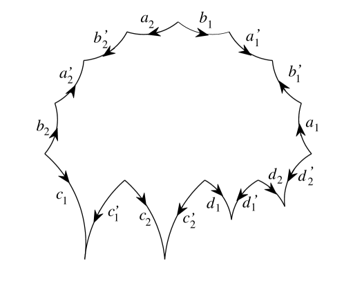
Figure 1. The convention of the fundamental domain $F$.

According to the isomorphism $\mathsf{S}_{\bullet}\simeq\mathsf{K}_{\bullet,0}$, the fundamental domain $F$ is identified with $F\otimes[\;]\in\mathsf{K}_{2,0}$. We have $\partial^{\prime\prime}F=0$, and it follows from (2.5) that

$$\begin{split}\partial^{\prime}F=&\sum_{k=1}^{g}\left(\beta_{k}^{-1}\left(b_{k}\right)-b_{k}-\alpha_{k}^{-1}\left(a_{k}\right)+a_{k}\right)-\sum_{i=1}^{n}\left(\kappa_{i}^{-1}\left(c_{i}\right)-c_{i}\right)\\ &-\sum_{j=1}^{r}\left(\tau_{j}^{-1}\left(d_{j}\right)-d_{j}\right)\\ =&\partial^{\prime\prime}L,\end{split}$$

where $L\in\mathsf{K}_{1,1}$ is given by

$$L=\sum_{k=1}^{g}\left(b_{k}\otimes\left[\beta_{k}\right]-a_{k}\otimes\left[\alpha_{k}\right]\right)-\sum_{i=1}^{n}c_{i}\otimes\left[\kappa_{i}\right]-\sum_{j=1}^{r}d_{j}\otimes\left[\tau_{j}\right].$$ (2.6)

There exists $V\in\mathsf{K}_{0,2}$ such that

$$\partial^{\prime}L=\partial^{\prime\prime}V-\sum_{i=1}^{n}x_{i}\otimes[\kappa_{i}]-\sum_{j=1}^{r}z_{j}\otimes[\tau_{j}].$$ (2.7)

Here $x_{i}=c_{i}(1)$ are representatives of the punctures of the Riemann surface $X=\Gamma\backslash\mathbb{U}$ on $\mathbb{R}\cup\{\infty\}$ and $z_{j}=d_{j}(1)$ are representatives of the ramification points of $X$ on $\mathbb{U}$. In the presence of ramification points, the expression for $V$ is much more complicated. One can verify that it is given by

$$\begin{split}V&=\sum_{k=1}^{g}\left(a_{k}(0)\otimes[\alpha_{k}|\beta_{k}]-b_{k}(0)\otimes\left[\beta_{k}|\alpha_{k}\right]+b_{k}(0)\otimes\left[\gamma_{k}^{-1}|\alpha_{k}\beta_{k}\right]\right)\\ &\;\;\;-\sum_{k=1}^{g-1}b_{g}(0)\otimes\left[\gamma_{g}^{-1}\ldots\gamma_{k+1}^{-1}|\gamma_{k}^{-1}\right]\\ &+\sum_{i=1}^{n-1}c_{1}(0)\otimes\left[\kappa_{1}\cdots\kappa_{i}|\kappa_{i+1}\right]+\sum_{j=0}^{r-1}c_{1}(0)\otimes\left[\kappa_{1}\ldots\kappa_{n}\tau_{1}\cdots\tau_{j}|\tau_{j+1}\right].\end{split}$$ (2.8)

Define

$$\Sigma=F+L-V.$$

Then

$$\partial\Sigma=-\sum_{i=1}^{n}x_{i}\otimes[\kappa_{i}]-\sum_{j=1}^{r}z_{j}\otimes[\tau_{j}].$$

When $\Gamma$ contains parabolic or elliptic elements, $\Sigma$ is not a cycle.

Finally, we also define $W$ in the following way. Let $P_{k}$ be a $\Gamma$-contracting path (see [9] for the definition of $\Gamma$-contractible) connecting 0 to $b_{k}(0)$. Then

$$\begin{split}W=&\sum_{k=1}^{g}\left(P_{k-1}\otimes\left[\alpha_{k}|\beta_{k}\right]-P_{k}\otimes\left[\beta_{k}|\alpha_{k}\right]+P_{k}\otimes\left[\gamma_{k}^{-1}|\alpha_{k}\beta_{k}\right]\right)\\ &-\sum_{k=1}^{g-1}P_{g}\otimes\left[\gamma_{g}^{-1}\ldots\gamma_{k+1}^{-1}|\gamma_{k}^{-1}\right]+\sum_{i=1}^{n-1}P_{g}\otimes\left[\kappa_{1}\ldots\kappa_{i}|\kappa_{i+1}\right]\\ &+\sum_{j=0}^{r-1}P_{g}\otimes\left[\kappa_{1}\ldots\kappa_{n}\tau_{1}\ldots\tau_{j}|\tau_{j+1}\right].\end{split}$$

If $\Gamma$ is a quasi-Fuchsian group, let $\Gamma_{1}$ be the Fuchsian group such that $\Gamma_{1}=J_{1}^{-1}\circ\Gamma\circ J_{1}$. The double complex associated with $\Omega=\Omega_{1}\sqcup\Omega_{2}$ and the group $\Gamma$ is a push-forward by the map $J_{1}$ of the double complex associated with $\mathbb{U}\sqcup\mathbb{L}$ and the group $\Gamma_{1}$.

$$\Sigma_{1}= J_{1}(\Sigma)=F_{1}+L_{1}-V_{1},$$

$$\Sigma_{2}= J_{1}\left(\bar{\Sigma}\right)=F_{2}+L_{2}-V_{2},$$

where $F_{1}=J_{1}(F)$, $F_{2}=J_{1}(\bar{F})$, $L_{1}=J_{1}(L)$, $L_{2}=J_{1}(\bar{L})$, $V_{1}=J_{1}(V)$, $V_{2}=J_{1}(\bar{V})$. Note that $\Sigma_{1}-\Sigma_{2}$ is a cycle only when there is no elliptic elements in $\Gamma$. In the general case we consider in this paper, $\Sigma_{1}-\Sigma_{2}$ is not a cycle.

2.2. Cohomology construction

The corresponding double complex in cohomology $\mathsf{C}^{\bullet,\bullet}$ is defined as $\mathsf{C}^{p,q}=\text{Hom}_{\mathbb{C}}\left(\mathsf{B}_{q},\mathsf{A}^{p}\right)$, where $\mathsf{A}^{\bullet}$ is the complexified de Rham complex on $\Omega=\Omega_{1}\sqcup\Omega_{2}$. The associated total complex $\text{Tot}\mathsf{C}$ is equipped with the total differential $D=d+(-1)^{p}\delta$ on $\mathsf{C}_{p,q}$, where $d$ is the de Rham differential and $\delta$ is the group coboundary. The natural pairing $\langle\;,\;\rangle$ between $\mathsf{C}^{p,q}$ and $\mathsf{K}_{p,q}$ is given by the integration over chains.

Let $\varphi=\phi_{\text{hyp}}$, where $e^{\phi_{\text{hyp}(z)}}|dz|^{2}$ is the hyperbolic metric on $\Omega$ given by (2.2). Denote by $\mathcal{CM}(X\sqcup Y)$ the space of conformal metrics on $\Gamma\backslash\Omega=X\sqcup Y$ satisfying certain regularity conditions at the parabolic and elliptic fixed points of $\Gamma$. That is, every $ds^{2}\in\mathcal{CM}(X\sqcup Y)$ is represented as $ds^{2}=e^{\phi(z)}|dz|^{2}$, where $\phi$ is a smooth function on $\Omega$ satisfying

$$\phi\circ\gamma+\log|\gamma^{\prime}|^{2}=\phi\quad\quad\forall\;\gamma\in\Gamma,$$

and

$$\phi(z)-\varphi(z)=O(1)$$

as $z$ approaches the parabolic and elliptic fixed points of $\Gamma$. Since $J^{-1}$ is univalent on $\Omega_{1}\sqcup\Omega_{2}$, from (2.2), we find that $\varphi(z)$ is regular when $z$ approaches the elliptic fixed points, and so does $\phi(z)$.

The Liouville action is a function on the space of conformal metrics. Its construction is as follows. Starting with the 2-form

$$\omega[\phi]=\left(|\phi_{z}|^{2}+e^{\phi}\right)dz\wedge d\bar{z}\in\mathsf{C}^{2,0},$$ (2.9)

we have

$$\delta\omega[\phi]=d\check{\theta}[\phi],$$

where $\check{\theta}[\phi]\in\mathsf{C}^{1,1}$ is given explicitly by

$$\check{\theta}_{\gamma^{-1}}[\phi]=\left(\phi-\frac{1}{2}\log|\gamma^{\prime}|^{2}-2\log 2-\log|c(\gamma)|^{2}\right)\left(\frac{\gamma^{\prime\prime}}{\gamma^{\prime}}dz-\frac{\overline{\gamma^{\prime\prime}}}{\overline{\gamma^{\prime}}}d\bar{z}\right).$$ (2.10)

Here $c(\gamma)$ is the element $c$ in the linear fractional transformation $\displaystyle\gamma=\begin{pmatrix}a&b\\ c&d\end{pmatrix}.$ Notice that $\check{\theta}_{\gamma^{-1}}[\phi]=0$ if $c(\gamma)=0$.

Next, set

$$\check{u}=\delta\check{\theta}[\phi]\in\mathsf{C}^{1,2}.$$

From the definition of $\check{\theta}$ and $\delta^{2}=0$, it follows that the 1-form $\check{u}$ is closed. An explicit calculation gives

$$\begin{split}\check{u}_{\gamma_{1}^{-1},\gamma_{2}^{-1}}=&-\left(\frac{1}{2}\log|\gamma_{1}^{\prime}|^{2}+\log\frac{|c(\gamma_{2})|^{2}}{|c(\gamma_{2}\gamma_{1})|^{2}}\right)\left(\frac{\gamma_{2}^{\prime\prime}}{\gamma_{2}^{\prime}}\circ\gamma_{1}\,\gamma_{1}^{\prime}\,dz-\frac{\overline{\gamma_{2}^{\prime\prime}}}{\overline{\gamma_{2}^{\prime}}}\circ\gamma_{1}\,\overline{\gamma_{1}^{\prime}}\,d\bar{z}\right)\\ &+\left(\frac{1}{2}\log|\gamma_{2}^{\prime}\circ\gamma_{1}|^{2}+\log\frac{|c(\gamma_{2}\gamma_{1})|^{2}}{|c(\gamma_{1})|^{2}}\right)\left(\frac{\gamma_{1}^{\prime\prime}}{\gamma_{1}^{\prime}}dz-\frac{\overline{\gamma_{1}^{\prime\prime}}}{\overline{\gamma_{1}^{\prime}}}d\bar{z}\right).\end{split}$$

Remark 2.1.

Notice that for a linear transformation $\gamma$,

$$-2c(\gamma)=\frac{\gamma^{\prime\prime}(z)}{\left(\gamma^{\prime}(z)\right)^{\frac{3}{2}}}.$$ (2.11)

Hence, $\check{\theta}_{\gamma^{-1}}[\phi]$ and $\check{u}_{\gamma_{1}^{-1},\gamma_{2}^{-1}}$ can be rewritten as

$$\check{\theta}_{\gamma^{-1}}[\phi]=\left(\phi-\log\left|\frac{\gamma^{\prime\prime}}{\gamma^{\prime}}\right|^{2}\right)\left(\frac{\gamma^{\prime\prime}}{\gamma^{\prime}}dz-\frac{\overline{\gamma^{\prime\prime}}}{\overline{\gamma^{\prime}}}d\bar{z}\right),$$ (2.12)

$$\begin{split}\check{u}_{\gamma_{1}^{-1},\gamma_{2}^{-1}}=&-\left(\log\left|\frac{\gamma_{2}^{\prime\prime}}{\gamma_{2}^{\prime}}\circ\gamma_{1}\right|^{2}\right)\left(\frac{\gamma_{2}^{\prime\prime}}{\gamma_{2}^{\prime}}\circ\gamma_{1}\,\gamma_{1}^{\prime}\,dz-\frac{\overline{\gamma_{2}^{\prime\prime}}}{\overline{\gamma_{2}^{\prime}}}\circ\gamma_{1}\,\overline{\gamma_{1}^{\prime}}\,d\bar{z}\right)\\ &+\left(\log\left|\frac{(\gamma_{2}\circ\gamma_{1})^{\prime\prime}}{(\gamma_{2}\circ\gamma_{1})^{\prime}}\right|^{2}\right)\left(\frac{(\gamma_{2}\circ\gamma_{1})^{\prime\prime}}{(\gamma_{2}\circ\gamma_{1})^{\prime}}dz-\frac{\overline{(\gamma_{2}\circ\gamma_{1})^{\prime\prime}}}{\overline{(\gamma_{2}\circ\gamma_{1})^{\prime}}}d\bar{z}\right)\\ &-\left(\log\left|\frac{\gamma_{1}^{\prime\prime}}{\gamma_{1}^{\prime}}\right|^{2}\right)\left(\frac{\gamma_{1}^{\prime\prime}}{\gamma_{1}^{\prime}}dz-\frac{\overline{\gamma_{1}^{\prime\prime}}}{\overline{\gamma_{1}^{\prime}}}d\bar{z}\right).\end{split}$$ (2.13)

For $e^{\phi(z)}|dz|^{2}\in\mathcal{CM}(X\sqcup Y)$, the Liouville action is defined as

$$S[\phi]= \frac{i}{2}\Bigl{(}\langle\omega[\phi],F_{1}-F_{2}\rangle-\langle\check{\theta}[\phi],L_{1}-L_{2}\rangle+\langle\check{u},W_{1}-W_{2}\rangle\Bigr{)},$$ (2.14)

where $W_{1}=J_{1}(W)$ and $W_{2}=J_{1}(\bar{W})$. When $e^{\phi}=e^{\varphi}$ is the hyperbolic metric, $S[\varphi]$ is well-defined by Theorem A.5. For a conformal metric $e^{\phi(z)}|dz|^{2}\in\mathcal{CM}(X\sqcup Y)$, $S[\phi]$ is also well-defined since $\phi(z)-\varphi(z)=O(1)$ as $z$ approaches the parabolic and elliptic fixed points.

Remark 2.2.

When $\Gamma$ contains elliptic elements, $\Sigma_{1}-\Sigma_{2}$ is not a cycle. Hence, it is not clear that the Liouville action defined above is independent of the choice of fundamental domains. By Theorem 4.8, the Liouville action is equal to the renormalized volume of the corresponding hyperbolic three-manifold defined by $\Gamma$ up to some constants. This shows that the Liouville action is indeed independent of the choice of fundamental domain.

Remark 2.3.

In [9], the Liouville action was originally defined by

$$S[\phi]=\frac{i}{2}\Bigl{(}\langle\omega[\phi],F_{1}-F_{2}\rangle-\langle\check{\theta}[\phi],L_{1}-L_{2}\rangle+\langle\check{\Theta},V_{1}-V_{2}\rangle\Bigr{)}$$ (2.15)

where $\check{\Theta}\in\mathsf{C}^{0,2}$ with $d\check{\Theta}=\check{u}$. It can be shown that the definition in (2.15) is equivalent to the definition in (2.14) by

$$\langle\check{u},W_{1}-W_{2}\rangle= \langle d\check{\Theta},W_{1}-W_{2}\rangle=\langle\check{\Theta},\partial^{\prime}(W_{1}-W_{2})\rangle=\langle\check{\Theta},V_{1}-V_{2}\rangle$$

where we used $\partial^{\prime}(W_{1}-W_{2})=V_{1}-V_{2}$.

2.3. Classical Liouville action for Fuchsian groups

Let $e^{\varphi(z)}|dz|^{2}$ be the hyperbolic metric on $\Omega=\Omega_{1}\sqcup\Omega_{2}$. The critical point of the Liouville action along a conformal family of metrics appears at the hyperbolic metric. We call

$$S=S[\varphi]= \frac{i}{2}\Bigl{(}\langle\omega,F_{1}-F_{2}\rangle-\langle\check{\theta},L_{1}-L_{2}\rangle+\langle\check{u},W_{1}-W_{2}\rangle\Bigr{)}$$

the classical Liouville action. Here,

$$\omega=\omega[\varphi],\hskip 28.45274pt\check{\theta}=\check{\theta}[\varphi].$$

Let us consider the case where $\Gamma$ is a Fuchsian group. In [9] we prove that if $\Gamma$ is a cocompact Fuchsian group, then the classical Liouville action is equal to $8\pi(2g-2)$, where $g$ is the genus of the compact Riemann surface $\Gamma\backslash\mathbb{U}$. In other words,

$$S=8\pi\chi(X)$$

when $\Gamma\backslash\mathbb{U}\simeq X$ is a compact Riemann surface. It is natural to ask whether this is still true when $\Gamma\backslash\mathbb{U}\simeq X$ is a surface of type $(g,n;m_{1},m_{2},\ldots,m_{r})$.

When $\Gamma$ is a Fuchsian group,

$$\omega=2e^{\varphi}dz\wedge d\bar{z},$$

so that $\delta\omega=0$. Hence $d\check{\theta}=0$. This implies that $\check{\theta}=d\varkappa$ for some $\varkappa$. It follows that

$$\langle\check{u},W_{1}-W_{2}\rangle=\langle\delta d\varkappa,W_{1}-W_{2}\rangle=\langle\delta\varkappa,V_{1}-V_{2}\rangle=\langle\varkappa,\partial^{\prime\prime}(V_{1}-V_{2})\rangle.$$

Applying the equality of (2.7) to the double complex associated to the action of the Fuchsian group on $\mathbb{U}\sqcup\mathbb{L}$, we find that

$$\partial^{\prime}L_{1}-\partial^{\prime}L_{2}=\ \partial^{\prime\prime}V_{1}-\sum_{i=1}^{n}v_{i}\otimes[\kappa_{i}]-\sum_{j=1}^{r}z_{j}\otimes[\tau_{j}]$$

$$-\partial^{\prime\prime}V_{2}+\sum_{i=1}^{n}v_{i}\otimes[\kappa_{i}]+\sum_{j=1}^{r}\bar{z}_{j}\otimes[\tau_{j}]$$

$$=\ \partial^{\prime\prime}V_{1}-\partial^{\prime\prime}V_{2}-\sum_{j=1}^{r}\left(z_{j}-\bar{z}_{j}\right)\otimes[\tau_{j}].$$ (2.16)

Hence,

$$\langle\check{u},W_{1}-W_{2}\rangle=\langle\check{\theta},L_{1}-L_{2}\rangle+\sum_{j=1}^{r}\langle\varkappa,\left(z_{j}-\bar{z}_{j}\right)\otimes[\tau_{j}]\rangle.$$

Therefore, when $\Gamma$ is a Fuchsian group, the classical Liouville action is given by

$$S=2\iint_{X\sqcup\bar{X}}e^{\varphi}d^{2}z+\frac{i}{2}\sum_{j=1}^{r}\langle\varkappa,\left(z_{j}-\bar{z}_{j}\right)\otimes[\tau_{j}]\rangle.$$ (2.17)

This shows that when $\Gamma$ does not contain elliptic elements, we indeed have $S=8\pi\chi(X).$ When $\Gamma$ contains elliptic elements, there is an additional term given by

$$\frac{i}{2}\sum_{j=1}^{r}\langle\varkappa,\left(z_{j}-\bar{z}_{j}\right)\otimes[\tau_{j}]\rangle.$$

Let us compute this term. By the definition of $\varkappa$, we have

$$\langle\varkappa,\left(z_{j}-\bar{z}_{j}\right)\otimes[\tau_{j}]\rangle= \varkappa_{\tau_{j}}(z_{j})-\varkappa_{\tau_{j}}(\bar{z}_{j})$$

$$= \int_{\bar{z}_{j}}^{z_{j}}\check{\theta}_{\tau_{j}}$$

$$= -\int_{\bar{z}_{j}}^{z_{j}}\left(\log y^{2}+\log\left|\frac{\tau_{j}^{-1\prime\prime}}{\tau_{j}^{-1\prime}}\right|^{2}\right)\left(\frac{\tau_{j}^{-1\prime\prime}}{\tau_{j}^{-1\prime}}dz-\frac{\overline{\tau_{j}^{-1\prime\prime}}}{\overline{\tau_{j}^{-1\prime}}}d\bar{z}\right).$$

Now $\tau_{j}=\rho_{j}\lambda_{m_{j}}\rho_{j}^{-1}$, where

$$\rho_{j}=\begin{pmatrix}-\varpi e^{-i\alpha}\bar{z}_{j}&\varpi e^{i\alpha}z_{j}\\ -\varpi e^{-i\alpha}&\varpi e^{i\alpha}\end{pmatrix},\qquad\lambda_{m_{j}}=\begin{pmatrix}e^{\frac{\pi i}{m_{j}}}&0\\ 0&e^{-\frac{\pi i}{m_{j}}}\end{pmatrix},$$ (2.18)

where $\alpha$ is a constant and $\varpi^{2}=(z_{j}-\bar{z}_{j})^{-1}$. Hence,

$$\tau_{j}^{-1}(z)=\frac{(z_{j}e^{i\beta}-\bar{z}_{j}e^{-i\beta})z-z_{j}\bar{z_{j}}(e^{i\beta}-e^{-i\beta})}{(e^{i\beta}-e^{-i\beta})z-(\bar{z}_{j}e^{i\beta}-z_{j}e^{-i\beta})},$$

where $\beta=\pi/m_{j}$. It follows that

$$\frac{\tau_{j}^{-1\prime\prime}(z)}{\tau_{j}^{-1\prime}(z)}=-\frac{2(e^{i\beta}-e^{-i\beta})}{(e^{i\beta}-e^{-i\beta})z-(\bar{z}_{j}e^{i\beta}-z_{j}e^{-i\beta})}.$$

We can choose the integration path from $\bar{z}_{j}$ to $z_{j}$ to be the straight line from $\bar{z}_{j}$ to $z_{j}$. Using the parametrization

$$s\in[-1,1]\quad\longrightarrow\quad z(s)=\frac{z_{j}+\bar{z}_{j}+s(z_{j}-\bar{z}_{j})}{2},$$

we find that

$$\langle\varkappa,\left(z_{j}-\bar{z}_{j}\right)\otimes[\tau_{j}]\rangle$$

$$= 2\int_{-1}^{1}\log\frac{s^{2}(4\sin^{2}\beta)}{\left|\cos\beta+is\sin\beta\right|^{2}}d\log\frac{\cos\beta+is\sin\beta}{\cos\beta-is\sin\beta}$$

$$= 4\int_{0}^{1}\log\frac{s^{2}(4\sin^{2}\beta)}{\left|\cos\beta+is\sin\beta\right|^{2}}d\log\frac{\cos\beta+is\sin\beta}{\cos\beta-is\sin\beta}$$

$$= 8\int_{0}^{1}\log s\;d\log\frac{\cos\beta+is\sin\beta}{\cos\beta-is\sin\beta}+4\log\left(4\sin^{2}\beta\right)\int_{0}^{1}d\log\frac{\cos\beta+is\sin\beta}{\cos\beta-is\sin\beta}$$

$$-4\int_{0}^{1}\log\left|\cos\beta+is\sin\beta\right|^{2}d\log\frac{\cos\beta+is\sin\beta}{\cos\beta-is\sin\beta}$$

$$= (\text{I})+(\text{II})+(\text{III}).$$

Let us recall the dilogarithm function

$$\begin{split}\mathrm{Li}_{2}(z):=&-\int_{0}^{z}\frac{\log(1-t)}{t}\,dt\\ =&-\int_{0}^{1}\frac{\log(1-zt)}{t}dt\\ =&\int_{0}^{1}\log t\;\;d\log(1-zt).\end{split}$$ (2.19)

This gives

$$(\text{I})= 8\int_{0}^{1}\log s\;d\log\frac{1+is\tan\beta}{1-is\tan\beta}$$

$$= 8\text{Li}_{2}\left(-i\tan\beta\right)-8\text{Li}_{2}\left(i\tan\beta\right).$$

It is straightforward to find that

$$(\text{II})= 4\log\left(4\sin^{2}\beta\right)\int_{0}^{1}d\log\frac{\cos\beta+is\sin\beta}{\cos\beta-is\sin\beta}$$

$$= 8i\beta\log\left(4\sin^{2}\beta\right).$$

The computation of (III) is more complicated. It is given by the lemma below.

Lemma 2.4.

Let $x$ and $y$ be constants with $x>0$ and $x^{2}+y^{2}=1$. Then

$$\int_{0}^{1}\log|x+isy|^{2}d\log\frac{x+isy}{x-isy}$$

$$= \log(2x)\log\frac{x+iy}{x-iy}-\text{Li}_{2}\left(\frac{x+iy}{2x}\right)+\text{Li}_{2}\left(\frac{x-iy}{2x}\right).$$

Proof.

Let $u=x+isy$, $v=x-isy$. Then

$$I= \int_{0}^{1}\log|x+isy|^{2}\;d\log\frac{x+isy}{x-isy}$$

$$= \int_{0}^{1}\left(\log u\;d\log u+\log v\;d\log u-\log u\;d\log v-\log v\;d\log v\right).$$

On the other hand, integration by parts gives

$$I= -\int_{0}^{1}\log\frac{x+isy}{x-isy}\;d\log|x+isy|^{2}$$

$$= -\int_{0}^{1}\left(\log u\;d\log u+\log u\;d\log v-\log v\;d\log u-\log v\;d\log v\right).$$

It follows that

$$\int_{0}^{1}\left(\log u\;d\log u-\log v\;d\log v\right)=0$$

and

$$I= \int_{0}^{1}\left(\log v\;d\log u-\log u\;d\log v\right)$$

$$= \int_{0}^{1}\left(\log(x-isy)\;d\log(x+isy)-\log(x+isy)\;d\log(x-isy)\right).$$

Now

$$\int_{0}^{1}\log(x-isy)d\log(x+isy)= \int_{x}^{x+iy}\log(2x-t)\frac{dt}{t}$$

$$= \int_{\frac{1}{2}}^{\frac{x+iy}{2x}}\left(\log(2x)+\log(1-t)\right)\frac{dt}{t}$$

$$= \log(2x)\log\frac{x+iy}{x}-\text{Li}_{2}\left(\frac{x+iy}{2x}\right)+\text{Li}_{2}\left(\frac{1}{2}\right).$$

Changing $y$ to $-y$ gives

$$\int_{0}^{1}\log(x+isy)d\log(x-isy)= \log(2x)\log\frac{x-iy}{x}-\text{Li}_{2}\left(\frac{x-iy}{2x}\right)+\text{Li}_{2}\left(\frac{1}{2}\right).$$

It follows that

$$\int_{0}^{1}\log|x+isy|^{2}d\log\frac{x+isy}{x-isy}$$

$$= \log(2x)\log\frac{x+iy}{x-iy}-\text{Li}_{2}\left(\frac{x+iy}{2x}\right)+\text{Li}_{2}\left(\frac{x-iy}{2x}\right).$$

∎

From Lemma 2.4, we find that

$$(\text{III})= -4\int_{0}^{1}\log\left|\cos\beta+is\sin\beta\right|^{2}d\log\frac{\cos\beta+is\sin\beta}{\cos\beta-is\sin\beta}$$

$$= -8i\beta\log\left(2\cos\beta\right)+4\text{Li}_{2}\left(\frac{1}{1+e^{-2i\beta}}\right)-4\text{Li}_{2}\left(\frac{1}{1+e^{2i\beta}}\right).$$

Hence,

$$\langle\varkappa,\left(z_{j}-\bar{z}_{j}\right)\otimes[\tau_{j}]\rangle$$

$$= 8\text{Li}_{2}\left(-i\tan\beta\right)-8\text{Li}_{2}\left(i\tan\beta\right)+8i\beta\log\left(4\sin^{2}\beta\right)$$

$$-8i\beta\log\left(2\cos\beta\right)+4\text{Li}_{2}\left(\frac{1}{1+e^{-2i\beta}}\right)-4\text{Li}_{2}\left(\frac{1}{1+e^{2i\beta}}\right)$$

$$= -16i\;\mathrm{Im}\text{Li}_{2}\left(i\tan\beta\right)+8i\;\mathrm{Im}\text{Li}_{2}\left(\frac{1}{1+e^{-2i\beta}}\right)+8i\beta\log\frac{2\sin^{2}\beta}{\cos\beta}.$$

Now let us recall that the Bloch-Wigner function $D(z)$ is given by [13]:

$$D(z)=\mathrm{Im}\left(\mathrm{Li}_{2}(z)\right)+\mathrm{arg}(1-z)\log|z|\qquad\text{for}\quad z\in\mathbb{C}.$$ (2.20)

Since

$$\log|i\tan\beta|=\log\frac{\sin\beta}{\cos\beta},\hskip 28.45274pt\log\left|\frac{1}{1+e^{-2i\beta}}\right|=-\log(2\cos\beta),$$

$$\mathrm{arg}(1-i\tan\beta)=-\beta,\hskip 28.45274pt\mathrm{arg}\left(1-\frac{1}{1+e^{-2i\beta}}\right)=-\beta,$$

we find that

$$\begin{split}&\langle\varkappa,\left(z_{j}-\bar{z}_{j}\right)\otimes[\tau_{j}]\rangle\\ =&-16i\;\left(D\left(i\tan\beta\right)+\beta\log\frac{\sin\beta}{\cos\beta}\right)+8i\;\left(D\left(\frac{1}{1+e^{-2i\beta}}\right)-\beta\log(2\cos\beta)\right)\\ &+8i\beta\log\frac{2\sin^{2}\beta}{\cos\beta}\\ =&-16i\,D\left(i\tan\beta\right)+8i\,D\left(\frac{1}{1+e^{-2i\beta}}\right).\end{split}$$ (2.21)

Using the identity (see [13])

$$D(z)=\frac{1}{2}\left[D\left(\frac{z}{\bar{z}}\right)+D\left(\frac{1-1/z}{1-1/\bar{z}}\right)+D\left(\frac{1/(1-z)}{1/(1-\bar{z})}\right)\right],$$

we find that

$$D(i\tan\beta)=\frac{1}{2}\left[D(-1)+D(-e^{-2i\beta})+D(e^{2i\beta})\right].$$

By definition,

$$D\left(e^{i\theta}\right)=\sum_{n=1}^{\infty}\frac{\sin n\theta}{n^{2}}.$$

Hence, $D(-1)=0$. On the other hand, we also have the identity (see [13])

$$D(z)=D\left(1-\frac{1}{z}\right).$$

Hence,

$$D\left(\frac{1}{1+e^{-2i\beta}}\right)=D(-e^{-2i\beta}).$$

Therefore,

$$\langle\varkappa,\left(z_{j}-\bar{z}_{j}\right)\otimes[\tau_{j}]\rangle=-8i\,D(e^{2i\beta}).$$

Gathering the results above, we have

Theorem 2.5.

When $\Gamma$ is a Fuchsian group of type $(g;n;m_{1},m_{2},\ldots,m_{r})$, the classical Liouville action $S$ is given by

$$S=8\pi\chi(X)+4\sum_{j=1}^{r}D\left(e^{\frac{2\pi i}{m_{j}}}\right),$$

where $\chi(X)$ is given by (2.1).

3. Variations of the classical Liouville action

In this section, we want to compute the first and second variations of the classical Liouville action on $\mathfrak{D}(\Gamma)$. Most of the computations are similar to the one given in [9] when $\Gamma$ does not contain parabolic or elliptic elements. However, we have to be careful when analysing the possible singularities at the parabolic and elliptic fixed points. There might also be extra terms appearing at the elliptic fixed points since the double complex $\Sigma_{1}-\Sigma_{2}$ is not a cycle.

Given a harmonic Beltrami differential $\mu$, let $f^{\mu}$ be the unique quasi-conformal mapping with Beltrami differential $\mu$ that fixes the points $0,1,\infty$. Notice that $f^{\varepsilon\mu}$ varies holomorphically with respect to $\varepsilon$ and thus

$$\left.\frac{\partial}{\partial\bar{\varepsilon}}f^{\varepsilon\mu}\right|_{\varepsilon=0}=0.$$

Let

$$\dot{f}=\left.\frac{\partial}{\partial\varepsilon}f^{\varepsilon\mu}\right|_{\varepsilon=0}.$$

It follows from the definition

$$f^{\varepsilon\mu}_{\bar{z}}=\varepsilon\mu f^{\varepsilon\mu}_{z}$$

that

$$\dot{f}_{\bar{z}}=\mu.$$

For any linear fractional transformation $\gamma$, let

$$\gamma^{\varepsilon\mu}=f^{\varepsilon\mu}\circ\gamma\circ(f^{\varepsilon\mu})^{-1}.$$

Then $\gamma^{\varepsilon\mu}$ varies holomorphically with respect to $\varepsilon$ . We collect some formulas in the following theorem.

Lemma 3.1.

Let $\mu$ be a harmonic Beltrami differential of $\Gamma$. On $\mathfrak{D}(\Gamma)$, we have the following variation formulas:

1. $\displaystyle\left.\frac{\partial}{\partial\varepsilon}\left(e^{\varphi^{\varepsilon\mu}\circ f^{\varepsilon\mu}}\left|f_{z}^{\varepsilon\mu}\right|^{2}\right)\right|_{\varepsilon=0}=0$,

2. $\displaystyle\left.\frac{\partial}{\partial\varepsilon}\left(\varphi^{\varepsilon\mu}\circ f^{\varepsilon\mu}\right)\right|_{\varepsilon=0}=-\dot{f}_{z}$,

3. $\displaystyle\left.\frac{\partial}{\partial\varepsilon}\left(\varphi^{\varepsilon\mu}_{z}\circ f^{\varepsilon\mu}f_{z}^{\varepsilon\mu}\right)\right|_{\varepsilon=0}=-\dot{f}_{zz}$,

4. $\displaystyle\left.\frac{\partial}{\partial\varepsilon}\left(\varphi^{\varepsilon\mu}_{\bar{z}}\circ f^{\varepsilon\mu}\bar{f}_{\bar{z}}^{\varepsilon\mu}\right)\right|_{\varepsilon=0}=0$,

5. $\displaystyle\left.\frac{\partial}{\partial\varepsilon}\left(\log\left|\left(\gamma^{\varepsilon\mu}\right)^{\prime}\circ f^{\varepsilon\mu}\right|^{2}\right)\right|_{\varepsilon=0}=\dot{f}_{z}\circ\gamma-\dot{f}_{z}$,

6. $\displaystyle\left.\frac{\partial}{\partial\varepsilon}\left(\frac{\left(\gamma^{\varepsilon\mu}\right)^{\prime\prime}}{\left(\gamma^{\varepsilon\mu}\right)^{\prime}}\circ f^{\varepsilon\mu}f^{\varepsilon\mu}_{z}\right)\right|_{\varepsilon=0}=\dot{f}_{zz}\circ\gamma\gamma^{\prime}-\dot{f}_{zz}$,

7. $\displaystyle\left.\frac{\partial}{\partial\varepsilon}\left(\frac{\left(\gamma^{\varepsilon\mu}\right)^{\prime\prime}}{\left(\gamma^{\varepsilon\mu}\right)^{\prime}}\circ f^{\varepsilon\mu}\right)\right|_{\varepsilon=0}=\dot{f}_{zz}\circ\gamma\gamma^{\prime}-\dot{f}_{zz}-\frac{\gamma^{\prime\prime}}{\gamma^{\prime}}\dot{f}_{z}$.

Proof.

The proof of (i) follows from the classical result of Ahlfors [1]. The equalities (ii), (iii), (v) and (vi) are given in p.213-214 of [9]. For (iv), we start with the following equality given in (3.6) of [9]:

$$\left.\frac{\partial}{\partial\varepsilon}\left(\varphi^{\varepsilon\mu}_{\bar{z}}\circ f^{\varepsilon\mu}\bar{f}_{\bar{z}}^{\varepsilon\mu}\right)\right|_{\varepsilon=0}= -\left(\varphi_{z}\dot{f}_{\bar{z}}+\dot{f}_{z\bar{z}}\right)$$

$$= -\left(\varphi_{z}\mu+\mu_{z}\right).$$

Since $\mu$ is a harmonic Beltrami differential, i.e.,

$$\mu=e^{-\varphi}\bar{q}$$

for some holomorphic quadratic differential $q$, it follows immediately that

$$\varphi_{z}\mu+\mu_{z}=0,$$ (3.1)

and (iv) is proved. (vii) follows immediately from (vi). ∎

Lemma 3.2.

We have the following formulas:

$$\dot{f}_{zz}\circ\gamma\gamma^{\prime}-\dot{f}_{zz}=\frac{1}{2}\left(\dot{f}_{z}\circ\gamma+\dot{f}_{z}\right)\frac{\gamma^{\prime\prime}}{\gamma^{\prime}}+\frac{\dot{c}(\gamma)}{c(\gamma)}\frac{\gamma^{\prime\prime}}{\gamma^{\prime}}\,,$$ (3.2)

$$\dot{f}_{z\bar{z}}\circ\gamma\overline{\gamma^{\prime}}-\dot{f}_{z\bar{z}}=\dot{f}_{\bar{z}}\frac{\gamma^{\prime\prime}}{\gamma^{\prime}}\,.$$ (3.3)

Proof.

Here we give a proof for (3.2) that is much simpler than the one given in [9]. From (2.11), we have

$$\log|2c(\gamma)|^{2}=\log\left|\frac{\gamma^{\prime\prime}}{\gamma^{\prime}}\right|^{2}-\frac{1}{2}\log|\gamma^{\prime}|^{2}.$$

It follows from (vii) and (v) of Theorem 3.1 that

$$\frac{\dot{c}(\gamma)}{c(\gamma)}=\frac{\dot{f}_{zz}\circ\gamma\gamma^{\prime}-\dot{f}_{zz}-\displaystyle\frac{\gamma^{\prime\prime}}{\gamma^{\prime}}\dot{f}_{z}}{\displaystyle\frac{\gamma^{\prime\prime}}{\gamma^{\prime}}}-\frac{1}{2}\left(\dot{f}_{z}\circ\gamma-\dot{f}_{z}\right),$$

from which (3.2) follows immediately. The equation (3.3) follows immediately by differentiating the identity

$$\dot{f}_{\bar{z}}\circ\gamma\frac{\overline{\gamma^{\prime}}}{\gamma^{\prime}}=\dot{f}_{\bar{z}}$$

with respect to $z$. ∎

The Lie derivatives of the smooth family of $(l,m)$ tensors $\omega$ on $\mathfrak{D}(\Gamma)$ along the vector field determined by $\mu$ are defined as

$$L_{\mu}\omega= \left.\frac{\partial}{\partial\varepsilon}\right|_{\varepsilon=0}\omega^{\varepsilon\mu}\circ f^{\varepsilon\mu}(f^{\varepsilon\mu}_{z})^{l}\left(\overline{f^{\varepsilon\mu}_{z}}\right)^{m},$$

$$L_{\bar{\mu}}\omega= \left.\frac{\partial}{\partial\bar{\varepsilon}}\right|_{\varepsilon=0}\omega^{\varepsilon\mu}\circ f^{\varepsilon\mu}(f^{\varepsilon\mu}_{z})^{l}\left(\overline{f^{\varepsilon\mu}_{z}}\right)^{m}.$$

Let

$$\vartheta(z)= 2\varphi_{zz}-\varphi_{z}^{2}$$

$$= \begin{cases}2\mathcal{S}\left(J_{1}^{-1}\right)(z),\quad&\text{if}\quad z\in\Omega_{1}\\ 2\mathcal{S}\left(J_{2}^{-1}\right)(z),\quad&\text{if}\quad z\in\Omega_{2}\end{cases},$$

where

$$\mathcal{S}(h)= \left(\frac{h_{zz}}{h_{z}}\right)_{z}-\frac{1}{2}\left(\frac{h_{zz}}{h_{z}}\right)^{2}$$

$$= \frac{h_{zzz}}{h_{z}}-\frac{3}{2}\left(\frac{h_{zz}}{h_{z}}\right)^{2}$$

is the Schwarzian derivative of $h$.

Theorem 3.3.

On the deformation space $\mathfrak{D}(\Gamma)$,

$$L_{\mu}S=\iint\limits_{\Gamma\backslash\Omega}\vartheta(z)\mu(z)d^{2}z.$$

Equivalently,

$$\partial S=\vartheta.$$

Proof.

By definition,

$$L_{\mu}S= \frac{i}{2}\Bigl{(}\langle L_{\mu}\omega,F_{1}-F_{2}\rangle-\langle L_{\mu}\check{\theta},L_{1}-L_{2}\rangle+\langle L_{\mu}\check{u},W_{1}-W_{2}\rangle\Bigr{)}.$$

As in p. 217 of [9], we find that

$$L_{\mu}\omega= -\varphi_{\bar{z}}\dot{f}_{zz}dz\wedge d\bar{z}$$

$$= \vartheta\mu dz\wedge d\bar{z}-d\xi,$$

where

$$\xi= 2\varphi_{z}\dot{f}_{\bar{z}}d\bar{z}-\varphi d\dot{f}_{z}=-2\dot{f}_{z\bar{z}}d\bar{z}-\varphi d\dot{f}_{z}.$$

Here we have used the equality (3.1). It follows that

$$\langle L_{\mu}\omega,F_{1}-F_{2}\rangle= \langle\vartheta\mu dz\wedge d\bar{z},F_{1}-F_{2}\rangle-\langle d\xi,F_{1}-F_{2}\rangle$$

$$= \langle\vartheta\mu dz\wedge d\bar{z},F_{1}-F_{2}\rangle-\langle\delta\xi,L_{1}-L_{2}\rangle.$$

The second equality follows from Theorem A.11 and

$$\partial^{\prime}(F_{1}-F_{2})=\partial^{\prime\prime}(L_{1}-L_{2}).$$

Now as in p.218 of [9], using the equality (3.3) we obtain

$$\delta\xi_{\gamma^{-1}}=-2\left(\dot{f}_{z\bar{z}}\circ\gamma\overline{\gamma^{\prime}}-\dot{f}_{z\bar{z}}\right)d\bar{z}-\varphi d\left(\dot{f}_{z}\circ\gamma-\dot{f}_{z}\right)+\log|\gamma^{\prime}|^{2}d\left(\dot{f}_{z}\circ\gamma\right).$$

Now, for the second term $\langle L_{\mu}\check{\theta},L_{1}-L_{2}\rangle$, by (v) of Lemma 3.1,

$$L_{\mu}\left(\varphi-\frac{1}{2}\log|\gamma^{\prime}|^{2}-2\log 2-\log|c(\gamma)|^{2}\right)$$

$$= -\dot{f}_{z}-\frac{1}{2}\left(\dot{f}_{z}\circ\gamma-\dot{f}_{z}\right)-\frac{\dot{c}(\gamma)}{c(\gamma)}=-\frac{1}{2}\left(\dot{f}_{z}\circ\gamma+\dot{f}_{z}\right)-\frac{\dot{c}(\gamma)}{c(\gamma)}$$

$$\hskip 150.79968pt=-\frac{\dot{f}_{zz}\circ\gamma\gamma^{\prime}-\dot{f}_{zz}}{\displaystyle\frac{\gamma^{\prime\prime}}{\gamma^{\prime}}}$$

where the last line follows from (3.2) and

$$L_{\mu}\left(\frac{\gamma^{\prime\prime}}{\gamma^{\prime}}dz-\frac{\overline{\gamma^{\prime\prime}}}{\overline{\gamma^{\prime}}}d\bar{z}\right)= L_{\mu}d\log|\gamma^{\prime}|^{2}=d\left(\dot{f}_{z}\circ\gamma-\dot{f}_{z}\right).$$

Hence,

$$L_{\mu}\check{\theta}_{\gamma^{-1}}= \left(\varphi-\frac{1}{2}\log|\gamma^{\prime}|^{2}-2\log 2-\log|c(\gamma)|^{2}\right)d\left(\dot{f}_{z}\circ\gamma-\dot{f}_{z}\right)$$

$$-\left(\frac{1}{2}\left(\dot{f}_{z}\circ\gamma+\dot{f}_{z}\right)+\frac{\dot{c}(\gamma)}{c(\gamma)}\right)\left(2\frac{\gamma^{\prime\prime}}{\gamma^{\prime}}dz-d\log|\gamma^{\prime}|^{2}\right)$$

$$= \left(\varphi-\frac{1}{2}\log|\gamma^{\prime}|^{2}-2\log 2-\log|c(\gamma)|^{2}\right)d\left(\dot{f}_{z}\circ\gamma-\dot{f}_{z}\right)$$

$$-2\left(\dot{f}_{zz}\circ\gamma\gamma^{\prime}-\dot{f}_{zz}\right)dz+\left(\frac{1}{2}\left(\dot{f}_{z}\circ\gamma+\dot{f}_{z}\right)+\frac{\dot{c}(\gamma)}{c(\gamma)}\right)d\log|\gamma^{\prime}|^{2}.$$

Let

$$\chi=\delta\xi+L_{\mu}\check{\theta}.$$

It follows that

$$\chi_{\gamma^{-1}}= dl_{\gamma^{-1}},$$

where

$$l_{\gamma^{-1}}= \frac{1}{2}\log|\gamma^{\prime}|^{2}\left(\dot{f}_{z}\circ\gamma+\dot{f}_{z}+2\frac{\dot{c}(\gamma)}{c(\gamma)}\right)$$

$$-\left(\log|c(\gamma)|^{2}+2+2\log 2\right)\left(\dot{f}_{z}\circ\gamma-\dot{f}_{z}\right).$$

By Lemma A.7 and Lemma A.10, $l_{\kappa_{i}}$ is well-defined when $z$ approaches the fixed point of $\kappa_{i}$ on $\mathcal{C}$. Hence, we have

$$\langle\delta\xi+L_{\mu}\check{\theta},L_{1}-L_{2}\rangle= \langle dl,L_{1}-L_{2}\rangle$$

$$= \langle l,\partial^{\prime}L_{1}-\partial^{\prime}L_{2}\rangle.$$

Since

$$L_{\mu}\check{u}= L_{\mu}\delta\check{\theta}=\delta L_{\mu}\check{\theta}=\delta\chi=\delta dl=d\delta l,$$

we have

$$\left\langle L_{\mu}\check{u},W_{1}-W_{2}\right\rangle= \left\langle\delta l,\partial^{\prime}(W_{1}-W_{2})\right\rangle$$

$$= \left\langle\delta l,V_{1}-V_{2}\right\rangle$$

$$= \left\langle l,\partial^{\prime\prime}V_{1}-\partial^{\prime\prime}V_{2}\right\rangle.$$

From this it follows that

$$L_{\mu}S=\frac{i}{2}\Bigl{(}\langle\vartheta\mu dz\wedge d\bar{z},F_{1}-F_{2}\rangle-\langle l,\partial^{\prime}L_{1}-\partial^{\prime}L_{2}-\partial^{\prime\prime}V_{1}+\partial^{\prime\prime}V_{2}\rangle\Bigr{)}.$$

Let $v_{i}\in\mathcal{C}$ be the fixed point of the parabolic generator $\kappa_{i}$, and let $\mathrm{w}_{1j}$ and $\mathrm{w}_{2j}$ be the fixed points of the elliptic generator $\tau_{j}$ in $\Omega_{1}$ and $\Omega_{2}$ respectively. Then

$$\partial^{\prime}L_{1}-\partial^{\prime}L_{2}= \partial^{\prime\prime}V_{1}-\sum_{i=1}^{n}v_{i}\otimes[\kappa_{i}]-\sum_{j=1}^{r}\mathrm{w}_{1j}\otimes[\tau_{j}]$$

$$-\partial^{\prime\prime}V_{2}+\sum_{i=1}^{n}v_{i}\otimes[\kappa_{i}]+\sum_{j=1}^{r}\mathrm{w}_{2j}\otimes[\tau_{j}]$$

$$= \partial^{\prime\prime}V_{1}-\partial^{\prime\prime}V_{2}-\sum_{j=1}^{r}\left(\mathrm{w}_{1j}-\mathrm{w}_{2j}\right)\otimes[\tau_{j}].$$

Hence,

$$L_{\mu}S= \frac{i}{2}\left(\langle\vartheta\mu dz\wedge d\bar{z},F_{1}-F_{2}\rangle+\left\langle l,\sum_{j=1}^{r}(\mathrm{w}_{1j}-\mathrm{w}_{2j})\otimes[\tau_{j}]\right\rangle\right).$$

Using Lemma A.6 and the fact that $\tau_{j}(\mathrm{w}_{1j})=\mathrm{w}_{1j}$, $\tau_{j}(\mathrm{w}_{2j})=\mathrm{w}_{2j}$, one finds that

$$\left\langle l,\sum_{j=1}^{r}(\mathrm{w}_{ij}-\mathrm{w}_{2j})\otimes[\tau_{j}]\right\rangle=0.$$

Hence, the presence of elliptic fixed points does not contribute additional terms. This concludes that

$$L_{\mu}S= \frac{i}{2}\langle\vartheta\mu dz\wedge d\bar{z},F_{1}-F_{2}\rangle,$$

which is the assertion of the theorem.

∎

Before going to the second variation, let us collect some additional variation formulas.

Lemma 3.4.

Let $\mu$ be a harmonic Beltrami differential of $\Gamma$. On $\mathfrak{D}(\Gamma)$, we have the following variation formulas:

1. $\displaystyle\left.\frac{\partial}{\partial\bar{\varepsilon}}\left(\varphi^{\varepsilon\mu}\circ f^{\varepsilon\mu}\right)\right|_{\varepsilon=0}=-\bar{\dot{f}}_{\bar{z}}$,

2. $\displaystyle\left.\frac{\partial}{\partial\bar{\varepsilon}}\left(\varphi^{\varepsilon\mu}_{z}\circ f^{\varepsilon\mu}f^{\varepsilon\mu}_{z}\right)\right|_{\varepsilon=0}=0$,

3. $\displaystyle\left.\frac{\partial}{\partial\bar{\varepsilon}}\left(\varphi^{\varepsilon\mu}_{zz}\circ f^{\varepsilon\mu}\left(f^{\varepsilon\mu}_{z}\right)^{2}\right)\right|_{\varepsilon=0}=-\frac{1}{2}e^{\varphi}\bar{\mu}$.

Proof.

(i) is the complex conjugate of the formula (ii) in Lemma 3.1. Differentiate this formula with respect to $z$, we have

$$\left.\frac{\partial}{\partial\bar{\varepsilon}}\left(\varphi^{\varepsilon\mu}_{z}\circ f^{\varepsilon\mu}f^{\varepsilon\mu}_{z}+\varphi^{\varepsilon\mu}_{\bar{z}}\circ f^{\varepsilon\mu}\overline{f^{\varepsilon\mu}}_{z}\right)\right|_{\varepsilon=0}=-\bar{\dot{f}}_{z\bar{z}}.$$

Using $\bar{\dot{f}}_{z}=\bar{\mu}$, we have

$$\left.\frac{\partial}{\partial\bar{\varepsilon}}\left(\varphi^{\varepsilon\mu}_{z}\circ f^{\varepsilon\mu}f^{\varepsilon\mu}_{z}\right)\right|_{\varepsilon=0}=-\bar{\mu}_{\bar{z}}-\varphi_{\bar{z}}\bar{\mu}=0.$$ (3.4)

The last equality follows from (3.1). Differentiating (3.4) again with respect to $z$, we have

$$\left.\frac{\partial}{\partial\bar{\varepsilon}}\left(\varphi^{\varepsilon\mu}_{zz}\circ f^{\varepsilon\mu}\left(f^{\varepsilon\mu}_{z}\right)^{2}+\varphi^{\varepsilon\mu}_{z\bar{z}}\circ f^{\varepsilon\mu}f^{\varepsilon\mu}_{z}\overline{f^{\varepsilon\mu}}_{z}+\varphi^{\varepsilon\mu}_{z}\circ f^{\varepsilon\mu}f^{\varepsilon\mu}_{z{z}}\right)\right|_{\varepsilon=0}=0.$$

This gives

$$\left.\frac{\partial}{\partial\bar{\varepsilon}}\left(\varphi^{\varepsilon\mu}_{zz}\circ f^{\varepsilon\mu}\left(f^{\varepsilon\mu}_{z}\right)^{2}\right)\right|_{\varepsilon=0}=-\varphi_{z\bar{z}}\bar{\mu}.$$

Then (iii) follows from the fact that the hyperbolic metric $e^{\varphi(z)}|dz|^{2}$ satisfies the Liouville equation

$$\varphi_{z\bar{z}}=\frac{1}{2}e^{-\varphi}.$$

∎

Theorem 3.5.

Let $\omega_{WP}$ be the symplectic form of the Weil-Petersson metric on $\mathfrak{D}(\Gamma)$. On $\mathfrak{D}(\Gamma)$,

$$d\vartheta=\bar{\partial}\partial S=-2i\omega_{WP}.$$

Hence, $-S$ is a Kähler potential of the Weil-Petersson metric on $\mathfrak{D}(\Gamma)$.

Proof.

By the definition of $\langle\,,\,\rangle_{\text{WP}}$ in (2.4), we need to show that

$$L_{\bar{\nu}}L_{\mu}S=-\iint\limits_{\Gamma\backslash\Omega}\mu(z)\overline{\nu(z)}\rho(z)d^{2}z.$$

Using the result of Theorem 3.3, the fact that $L_{\bar{\nu}}\mu=0$, as well as (ii) and (iii) in Lemma 3.4, we have

$$L_{\bar{\nu}}L_{\mu}S= \frac{i}{2}\left\langle L_{\bar{\nu}}\left(2\varphi_{zz}(z)-\varphi_{z}(z)^{2}\right)\mu dz\wedge d\bar{z},F_{1}-F_{2}\right\rangle$$

$$= -\iint\limits_{\Gamma\backslash\Omega}\mu(z)\overline{\nu(z)}\rho(z)d^{2}z.$$

The result follows.

∎

4. Renormalized volume of quasi-Fuchsian 3-manifold

The group $\text{PSL}(2,\mathbb{C})$ acts on the hyperbolic three space

$$\mathbb{U}^{3}=\{Z=(z,t)\,|\,z\in\mathbb{C},\;t>0\}$$

and its closure. Given $\displaystyle\gamma=\begin{pmatrix}a&b\\ c&d\end{pmatrix}\in\text{PSL}(2,\mathbb{C})$, let

$$J_{\gamma}(Z)=\frac{1}{|cz+d|^{2}+|ct|^{2}}.$$

Then $\gamma$ maps $Z$ to $\gamma Z$, where

$$z(\gamma Z)= \left((az+b)\overline{(cz+d)}+a\bar{c}t^{2}\right)J_{\gamma}(Z),$$

$$t(\gamma Z)= tJ_{\gamma}(Z).$$

Given a quasi-Fuchsian group $\Gamma\subset\text{PSL}(2,\mathbb{C})$, let $M=\Gamma\backslash\mathbb{U}^{3}$ be the quotient 3-manifold, which is called quasi-Fuchsian 3-manifold. The boundary of $M$ is $\partial^{\prime}M=X\sqcup Y\simeq\Gamma\backslash\Omega$. In this section, we want to define the renormalized volume of $M$ and prove its relation to the Liouville action.

4.1. Rank one cusps

Let $\zeta$ be a parabolic fixed point of a quasi-Fuchsian group $\Gamma$ and $Stab_{\zeta}$ be the parabolic subgroup fixing $\zeta$. We call $\zeta$ a rank one or two cusp if $Stab_{\zeta}$ has one or two generators respectively. From now on we consider only the rank one cusp.

The quotient of the horoball $\mathcal{H}_{s}=\{(z,t)\in\mathbb{U}^{3}\,|\,t\geq s\}$ by the rank one parabolic subgroup $Stab_{\zeta}$ may or may not be embedded in $M=\Gamma\backslash\mathbb{U}^{3}$. Once it is embedded for some $t=s_{0}$, it is also embedded for all larger values of $s_{0}$. In this case, the embedded image is the same as $\pi(\mathcal{H}_{s_{0}})$, where $\pi:\mathbb{U}^{3}\to M$ denotes the projection map. This subset is homeomorphic to $\{0<|z|\leq 1\}\times\mathbb{R}$. We refer to this as a solid cusp tube and its boundary $\pi(\partial\mathcal{H}_{s_{0}})$ as a cusp cylinder. A solid cusp tube has an infinite volume and a cusp cylinder has an infinite area. For a sufficiently large $s$, $\gamma(\mathcal{H}_{s})\cap\mathcal{H}_{s}=\varnothing$ for $\gamma\notin Stab_{\zeta}$, while $\gamma(\mathcal{H}_{s})=\mathcal{H}_{s}$ for $\gamma\in Stab_{\zeta}$.

A solid cusp tube is related to two punctures on the boundary $X\sqcup Y$. There exists a pair of punctures $p_{1}$ on $X$, $p_{2}$ on $Y$, uniquely associated with the conjugacy class of the rank one cusp. If $c_{1}$ in $X$, $c_{2}$ in $Y$ are small circles retractible to $p_{1}$, $p_{2}$ respectively, there is a pairing cylinder $C$ in $M$, which is a cylinder closed in $M$, and bounded by $c_{1}$, $c_{2}$. It bounds a subregion of $M$ called a solid pairing tube, which is homeomorphic to $C\times(0,1]$. The solid pairing tubes corresponding to the different conjugacy classes of rank one cusps can be chosen to be mutually disjoint in $M$. The circles $c_{1}$, $c_{2}$ can be chosen so that the pair lifts to a round circles in $\Omega$ mutually tangent at the fixed point $\zeta$. Such a pair of circles is called a double horocycle at $\zeta$.

Let us consider a special case when $\Gamma$ is a Fuchsian group. Suppose $\gamma_{0}:z\mapsto z+1$ is a generator of a rank one parabolic subgroup. Then $\{z\in\mathbb{C}\,|\,\mathrm{Im}(z)=\pm b\}$ for a constant $b>1$ is a double horocycle at the fixed point $\infty$. Let $P_{\pm}\subset\mathbb{U}^{3}$ denote the vertical planes rising from them and consider $Q=\{(z,t)\in\mathbb{U}^{3}\,|\,-b\leq\mathrm{Im}(z)\leq b,t>0\}$ they bound. Truncate $Q$ by the half space $K=\{(z,t)\in\mathbb{U}^{3}\,|\,t\geq a\}$ for a constant $a>1$. The relative boundary in $\mathbb{U}^{3}$ of the resulting tunnel $Q\setminus K$ projects to a pairing cylinder in $M$. We refer to the section 3.6 of [6] for more explanations about rank one cusps.

When the rank one cusp $v_{i}=\infty$ is associated to the parabolic subgroup generated by $\kappa_{i}=\begin{pmatrix}1&q_{i}\\ 0&1\end{pmatrix}$, we have

$$\sigma_{i}^{-1}\kappa_{i}\sigma_{i}=\begin{pmatrix}1&1\\ 0&1\end{pmatrix},\qquad\text{where}\quad\sigma_{i}=\begin{pmatrix}q_{i}^{\frac{1}{2}}&0\\ 0&q_{i}^{-\frac{1}{2}}\end{pmatrix},$$ (4.1)

and $\sigma_{i}$ maps a horoball $\mathcal{H}_{s}$ onto $\mathcal{H}_{|q_{i}|s}$. Hence, for $v_{i}=\infty$ with the associated parabolic element $\begin{pmatrix}1&q_{i}\\ 0&1\end{pmatrix}$, we define $\mathcal{H}_{i,\varepsilon}$ to be $\mathcal{H}_{|q_{i}|/\varepsilon}=\sigma_{i}(\mathcal{H}_{1/\varepsilon})$. When the rank one cusp $v_{i}$ is finite and associated with the parabolic subgroup generated by

$$\kappa_{i}=\begin{pmatrix}1+q_{i}v_{i}&-q_{i}v_{i}^{2}\\ q_{i}&1-q_{i}v_{i}\end{pmatrix},$$ (4.2)

we have

$$\sigma_{i}^{-1}\kappa_{i}\sigma_{i}=\begin{pmatrix}1&-1\\ 0&1\end{pmatrix},\qquad\text{where}\quad\sigma_{i}=\begin{pmatrix}q_{i}^{\frac{1}{2}}v_{i}&-q_{i}^{-\frac{1}{2}}\\ q_{i}^{\frac{1}{2}}&0\end{pmatrix}.$$ (4.3)

In this case,

Lemma 4.1.

For the element $\sigma_{i}\in PSL(2,\mathbb{C})$ and an open horoball $\mathcal{H}_{s}$, the image $\sigma_{i}(\mathcal{H}_{s})$ is an open horoball tangent to $\mathbb{C}$ at $\sigma_{i}(\infty)=v_{i}$ and with radius $(2|q_{i}|s)^{-1}$.

Proof.

It is well known that the image by $\sigma_{i}$ of an open horoball $\mathcal{H}_{s}$ is a open horoball tangent to $\mathbb{C}$. Hence, it is sufficient to find the tangency point of the horoball and its radius. For $Z=(z,t)$, the image of $\sigma_{i}$ in (4.3) of $Z$ is given by

$$\sigma_{i}(Z)=\left(v_{i}-\frac{1}{q_{i}}\,\frac{\bar{z}}{|z|^{2}+t^{2}},\quad\frac{1}{|q_{i}|}\,\frac{t}{|z|^{2}+t^{2}}\right).$$ (4.4)

Using this, one can check that for a fixed $x_{0}$ the image of a circle

$$\{(z,t)\in\mathbb{U}^{3}\,|z=x_{0}+iy,t=s\}\cup\{\infty\}$$

under $\sigma_{i}$ is a circle satisfying $|Z-Z_{0}|^{2}=(2|q_{i}|s)^{-2}$ where $Z_{0}=(v_{i},(2|q_{i}|s)^{-1})$. Moreover it is easy to check that this circle is tangent to $\mathbb{C}$ at $v_{i}$. The claim follows from this. ∎

Using Lemma 4.1, for finite $v_{i}$ we define $\mathcal{H}_{i,\varepsilon}$ to be the image by $\sigma_{i}$ of an open horoball $\mathcal{H}_{1/\varepsilon}$, which is an open horoball tangent to $\mathbb{C}$ at $\sigma_{i}(\infty)=v_{i}$ with radius ${\varepsilon}/{2|q_{i}|}$.

For $s\gg 0$, we consider $\mathcal{K}_{s}$ defined by

$$\mathcal{K}_{s}:=\{(z,t)\in\mathbb{U}^{3}\,|\,z=x+iy,|y|>s\}.$$

Note that the boundary of $\mathcal{H}_{s}\cup\mathcal{K}_{s}$ for $s\gg 0$ projects to a pairing cylinder in $M$ if $\infty$ is a rank one cusp. For $v_{i}=\infty$, we put $\mathcal{K}_{i,\varepsilon}$ to be $\mathcal{K}_{s}$ with $s=\varepsilon^{-1/2}$. For other finite $v_{i}$, we define $\mathcal{K}_{i,\varepsilon}$ to be the image by $\sigma_{i}$ of $\mathcal{K}_{s}$ with $s=\varepsilon^{-1/2}$.

4.2. Conical singularity

For an elliptic element $\tau_{j}$ of order $m_{j}$ with fixed points $\mathrm{w}_{1}$ and $\mathrm{w}_{2}$, we have that $\tau_{j}=\rho_{j}\lambda_{m_{j}}\rho_{j}^{-1}$, where

$$\rho_{j}=\begin{pmatrix}-\varpi e^{-i\alpha}\mathrm{w}_{2}&\varpi e^{i\alpha}\mathrm{w}_{1}\\ -\varpi e^{-i\alpha}&\varpi e^{i\alpha}\end{pmatrix},\qquad\lambda_{m_{j}}=\begin{pmatrix}e^{\frac{\pi i}{m_{j}}}&0\\ 0&e^{-\frac{\pi i}{m_{j}}}\end{pmatrix}$$ (4.5)

for some $\alpha$ and $\varpi^{2}=({\mathrm{w}_{1}-\mathrm{w}_{2}})^{-1}$. Note that the $t$-axis in $\mathbb{U}^{3}$ is fixed by $\lambda_{m_{j}}$ and it is mapped to the geodesic $h_{j}$ by $\rho_{j}$ which is a semicircle in $\mathbb{U}^{3}$ with two end points $\mathrm{w}_{1}$ and $\mathrm{w}_{2}$. We consider a neighborhood of the $t$-axis defined by

$$\mathcal{Q}_{\varepsilon}=\{(z,t)\in\mathbb{U}^{3}\,|\,t\geq\varepsilon^{-1}|z|\}.$$

Then the neighborhood $\mathcal{Q}_{\varepsilon}$ is mapped to a neighborhood $\mathcal{Q}_{j,\varepsilon}:=\rho_{j}(\mathcal{Q}_{\varepsilon})$ of the geodesic $h_{j}$. Note that this subset $\mathcal{Q}_{j,\varepsilon}$ is invariant under the action of $\tau_{j}$.

For a sufficiently small $\varepsilon>0$, the quotient of $\mathcal{Q}_{j,\varepsilon}$ by the finite group generated by $\tau_{j}$ can be embedded into $M$, and the images corresponding to pairs of elliptic fixed points can be mutually disjoint in $M$. The hyperbolic metric over these regions has the conical singularity of codimension $2$ since the angle around the projection image of the geodesic $h_{j}$ is $2\pi/m_{j}$.

Figure 2. $\mathcal{Q}_{\varepsilon}$ and $\mathcal{Q}_{j,\varepsilon}:=\rho_{j}(\mathcal{Q}_{\varepsilon})$.

A direct computation gives the following result.

Lemma 4.2.

For sufficiently small $\varepsilon>0$, two points $(0,\varepsilon)$ and $(0,\varepsilon^{-1})$ in the $t$-axis are mapped by $\rho_{j}$ to two points in the geodesic $h_{j}$ whose coordinates are given by

$$\rho_{j}\left((0,\varepsilon)\right)= \left(\mathrm{w}_{1}+(\mathrm{w}_{2}-\mathrm{w}_{1})\varepsilon^{2}+O(\varepsilon^{4}),\,|\mathrm{w}_{1}-\mathrm{w}_{2}|(\varepsilon-\varepsilon^{3})+O(\varepsilon^{5})\right),$$

$$\rho_{j}\left((0,\varepsilon^{-1})\right)= \left(\mathrm{w}_{2}+(\mathrm{w}_{1}-\mathrm{w}_{2})\varepsilon^{2}+O(\varepsilon^{4}),\,|\mathrm{w}_{1}-\mathrm{w}_{2}|(\varepsilon-\varepsilon^{3})+O(\varepsilon^{5})\right).$$

4.3. Chain complex of the quasi-Fuchsian 3-manifold

When $\Gamma$ is a Fuchsian group, we can choose a fundamental region $R$ for the action of $\Gamma$ in $\mathbb{U}^{3}$ in the following way. $R$ is bounded by the hemispheres which intersect $\hat{{\mathbb{C}}}$ along the circles that are orthogonal to $\mathbb{R}$ and bound the fundamental domain $F$. The fundamental region $R$ is a three-dimensional $CW$-complex with a single 3-cell given by the interior of $R$. The 2-cells — the faces $D_{k},D_{k}^{\prime},E_{k}$, $E_{k}^{\prime}$, $k=1,\dots,g$, $G_{i}$, $G_{i}^{\prime}$, $i=1,\ldots,n$, $H_{j}$, $H_{j}^{\prime}$, $j=1,\ldots,r$ are given by the parts of the boundary of $R$ bounded by the intersections of the hemispheres and the arcs $a_{k}-\bar{a}_{k}$, $a_{k}^{\prime}-\bar{a}_{k}^{\prime}$, $b_{k}-\bar{b}_{k}$, $b_{k}^{\prime}-\bar{b}_{k}^{\prime}$, $c_{i}-\bar{c}_{i}$, $c_{i}^{\prime}-\bar{c}_{i}^{\prime}$, $d_{j}-\bar{d}_{j}$, $d_{j}^{\prime}-\bar{d}_{j}^{\prime}$ respectively. The 1-cells — the edges, are given by the 1-cells of $F_{1}-F_{2}$ and by $e_{k}^{0},e^{1}_{k},f_{k}^{0},f^{1}_{k}$, $s_{k}$, $k=1,\dots,g$; $g_{i}^{0}$, $i=1,\ldots,n$ and $h_{j}^{0},h_{j}^{1}$, $j=1,\ldots,r$, defined as follows. The edges $e^{0}_{k}$ are intersections of the faces $E_{k-1}$ and $D_{k}$ joining the vertices $\bar{a}_{k}(0)$ to $a_{k}(0)$, the edges $e_{k}^{1}$ are intersections of the faces $D_{k}$ and $E_{k}^{\prime}$ joining the vertices $\bar{a}_{k}(1)$ to $a_{k}(1)$; $f^{0}_{k}=e^{0}_{k+1}$ are intersections of $E_{k}$ and $D_{k+1}$ joining $\bar{b}_{k}(0)$ to $b_{k}(0)$, $f_{k}^{1}$ are intersections of $D_{k}^{\prime}$ and $E_{k}$ joining $\bar{b}_{k}(1)$ to $b_{k}(1)$; $s_{k}$ are intersections of $E^{\prime}_{k}$ and $D^{\prime}_{k}$ joining $\bar{a}^{\prime}_{k}(1)$ to $a^{\prime}_{k}(1)$; $g_{j}^{0}$ are intersections of $G_{j-1}^{\prime}$ and $G_{j}$ joining $\bar{c}_{j}(0)$ to $c_{j}(0)$; $h_{j}^{0}$ are intersections of $H_{j-1}^{\prime}$ and $H_{j}$ joining $\bar{d}_{j}(0)$ to $d_{j}(0)$; and $h_{j}^{1}$ are intersections of $H_{j}^{\prime}$ and $H_{j}$ joining $\bar{d}_{j}(1)$ to $d_{j}(1)$. Finally, the 0-cells — the vertices, are given by the vertices of $F$. This property means that the edges of $R$ do not intersect in ${\mathbb{U}}^{3}$. When $\Gamma$ is a quasi-Fuchsian group, the fundamental region $R$ is a topological polyhedron homeomorphic to the geodesic polyhedron for the corresponding Fuchsian group.

As stated in p. 176 of [2] (this proof is given for a Riemann surface with punctures, but its proof works for our case verbatim), one can show that there exists an open set $\mathcal{O}$ in $\overline{\mathbb{U}^{3}}$ such that $R\subset\mathcal{O}$ and a function $\eta\in C^{\infty}\left(\mathbb{U}^{3}\cup\Omega\right)$ such that

1. $0<\eta<1$ and $\text{supp}\,\eta\subset\overline{\mathcal{O}}$.

2. For each $Z\in\mathbb{U}^{3}\cup\Omega$, there is a neighbourhood $U$ of $Z$ and a finite set $\Lambda$ of $\Gamma$ such that $\displaystyle\left.\eta\right|_{\gamma(U)}=0$ for each $\gamma\in\Gamma\setminus\Lambda$.

3. $\displaystyle\sum_{\gamma\in\Gamma}\eta(\gamma Z)=1$ for all $Z\in\mathbb{U}^{3}\cup\Omega$.

4. The only parabolic fixed points of $\Gamma$ that lie in $\overline{\mathcal{O}}$ are $v_{i}$, $i=1,\ldots,n$.

5. For a fixed constant $\varepsilon_{0}$, put the region $W_{i}:=\overline{\mathcal{O}}\cap\left(\mathcal{H}_{i,\varepsilon_{0}}\cup\mathcal{K}_{i,\varepsilon_{0}}\right)$. Then $\displaystyle\left.\eta\right|_{\gamma(W_{i})}=0$ for $\gamma\in\Gamma\setminus\{\text{id},\kappa_{i},\kappa_{i}^{-1}\}$, where $\kappa_{i}$ is the parabolic transformation with fixed point $v_{i}$.

For a given $ds^{2}=e^{\phi(z)}|dz|^{2}\in\mathcal{CM}(X\sqcup Y)$, we define

$$\hat{f}(z,t)=\begin{cases}te^{\phi(z)/2}\quad\text{for}\ (z,t)\in\overline{\mathcal{O}}\quad\text{and}\quad t\leq\varepsilon_{0}/2,\\ 1\qquad\quad\ \ \text{for}\ (z,t)\in\overline{\mathcal{O}}\quad\text{and}\quad t\geq\varepsilon_{0},\end{cases}$$

and extend it to be a smooth function $\hat{f}$ on $\overline{\mathcal{O}}$. Then let

$$f(Z)=\sum_{\gamma\in\Gamma}\eta(\gamma Z)\hat{f}(\gamma Z),$$

which is a $\Gamma$-automorphic function on $\cup_{\gamma\in\Gamma}\gamma R$. As in [9], one can show that

$$f(Z)=te^{\phi(z)/2}+O(t^{3})\qquad\text{as}\quad t\to 0$$

uniformly on compact subsets of $\cup_{\gamma\in\Gamma}\gamma R$. Note that we allow the case $v_{i}=\infty$ in the above construction of $f$. Near $\infty$ we have the following fact for $f$.

Lemma 4.3.

Over the set $\{(z,t)\in\mathcal{K}_{i,\varepsilon_{0}}\,|\,t\leq\varepsilon_{0}/2\}$ for a sufficiently small $\varepsilon_{0}>0$, the level defining function $f$ is given by $f(Z)=te^{\phi(z)/2}$.

Proof.

First, let us observe that

$$z(\gamma Z)=\frac{az+b}{d},\quad t(\gamma Z)=\frac{t}{|d|^{2}}$$

for a parabolic element $\gamma=\begin{pmatrix}a&b\\ 0&d\end{pmatrix}$. Hence, for the parabolic element $\gamma=\kappa_{i}^{\pm 1}$,

$$t(\gamma Z)e^{\phi(\gamma Z)/2}=t|d|^{-2}e^{\phi(\gamma z)/2}=te^{\phi(z)/2},$$

where we used $e^{\phi(\gamma z)/2}=e^{\phi(z)/2}|cz+d|^{2}$ at the second equality. Over the region $W_{i}\cap\{(z,t)\in\mathcal{K}_{i,\varepsilon_{0}}\,|\,t\leq\varepsilon_{0}/2\}$, we have $\eta|_{\gamma(W_{i})}=0$ for $\gamma\in\Gamma\setminus\{\mathrm{id},\kappa_{i},\kappa_{i}^{-1}\}$. Hence, for $Z\in\{(z,t)\in\mathcal{K}_{i,\varepsilon_{0}}\,|\,t\leq\varepsilon_{0}/2\}$,

$$f(Z)= \left(\eta\,t\,e^{\phi/2}\right)(Z)+\left(\eta\,t\,e^{\phi/2}\right)(\kappa_{i}Z)+\left(\eta\,t\,e^{\phi/2}\right)(\kappa_{i}^{-1}Z)$$

$$= \left(\eta(Z)+\eta(\kappa_{i}Z)+\eta(\kappa_{i}^{-1}Z)\right)\,t\,e^{\phi(z)/2}=te^{\phi(z)/2}.$$

∎

Due to the rank one cusps and conical singular lines, some arguments (for instance, the Stokes’ Theorem) do not work properly without truncating some parts near rank one cusps and conical singular lines. Hence, we truncate a noncompact domain $R$ using the level defining function $f$ near the bottom boundary of $R$ in addition to removing parts near rank one cusps and conical singularity lines as follows:

$$R_{\varepsilon}=R\cap\{f\geq\varepsilon\}\setminus\left(\cup_{i=1}^{n}\mathcal{P}_{i,\varepsilon}\cup_{j=1}^{r}\mathcal{Q}_{j,\varepsilon}\right),$$

where $\mathcal{P}_{i,\varepsilon}:=\mathcal{H}_{i,\varepsilon}\cup\mathcal{K}_{i,\varepsilon}$. By construction, we have

$$\gamma(R_{\varepsilon})=\gamma(R)\cap\gamma(\{f\geq\varepsilon\})\setminus\gamma\left(\cup_{i=1}^{n}\mathcal{P}_{i,\varepsilon}\cup_{j=1}^{r}\mathcal{Q}_{j,\varepsilon}\right)$$

for $\gamma\in\Gamma$. The boundary of $R_{\varepsilon}$ produced by truncations consists of

$$-F_{\varepsilon}=\partial^{\prime}R_{\varepsilon}\cap\{f=\varepsilon\},\quad T^{c}_{i,\varepsilon}:=\partial^{\prime}R_{\varepsilon}\cap\overline{\mathcal{P}}_{i,\varepsilon},\quad T^{e}_{j,\varepsilon}:=\partial^{\prime}R_{\varepsilon}\cap\overline{\mathcal{Q}}_{j,\varepsilon}.$$

Let us note that $T^{c}_{i,\varepsilon}$ projects to a subset in a pairing cylinder of the $i$-th rank one cusp corresponding to $v_{i}$. Hence the boundary of $R_{\varepsilon}$ is given by

$$\partial^{\prime}R_{\varepsilon}=-F_{\varepsilon} +\sum_{k=1}^{g}\left(D_{k,\varepsilon}-D_{k,\varepsilon}^{\prime}-E_{k,\varepsilon}+E_{k,\varepsilon}^{\prime}\right)$$

$$+\sum_{i=1}^{n}\left(G_{i,\varepsilon}-G_{i,\varepsilon}^{\prime}\right)+\sum_{i=1}^{n}T^{c}_{i,\varepsilon}$$

$$+\sum_{j=1}^{r}\left(H_{j,\varepsilon}-H_{j,\varepsilon}^{\prime}\right)+\sum_{j=1}^{r}T^{e}_{j,\varepsilon}.$$

Note that $D_{k,\varepsilon}$, $D_{k,\varepsilon}^{\prime}$, $E_{k,\varepsilon}$, $E_{k,\varepsilon}^{\prime}$ are truncated by removing parts $\{f<\varepsilon\}$, and that $G_{i,\varepsilon}$, $G_{i,\varepsilon}^{\prime}$ are truncated by removing parts $\{f<\varepsilon\}$ and $\mathcal{P}_{i,\varepsilon}$, $H_{j,\varepsilon}$, $H_{j,\varepsilon}^{\prime}$ are truncated by removing parts $\{f<\varepsilon\}$ and $\mathcal{Q}_{j,\varepsilon}$ respectively. Hence $G_{i,\varepsilon}$, $G_{i,\varepsilon}^{\prime}$ have a common boundary with $T^{c}_{i,\varepsilon}$, and $H_{j,\varepsilon}$, $H_{j,\varepsilon}^{\prime}$ have a common boundary with $T^{e}_{j,\varepsilon}$ respectively. Put $g^{1}_{i,\varepsilon}:=G_{i,\varepsilon}\cap T^{c}_{i,\varepsilon}$ so that $\kappa_{i}^{-1}g^{1}_{i,\varepsilon}=G_{i,\varepsilon}^{\prime}\cap T^{c}_{i,\varepsilon}$, and put $h^{1}_{j,\varepsilon}:=H_{j,\varepsilon}\cap T^{e}_{j,\varepsilon}$ so that $\tau_{j}^{-1}h^{1}_{j,\varepsilon}=H_{j,\varepsilon}^{\prime}\cap T^{e}_{j,\varepsilon}$. Let

$$B_{\varepsilon}=\sum_{k=1}^{g}\left(E_{k,\varepsilon}\otimes[\beta_{k}]-D_{k,\varepsilon}\otimes[\alpha_{k}]\right)-\sum_{i=1}^{n}G_{i,\varepsilon}\otimes[\kappa_{i}]-\sum_{j=1}^{r}H_{j,\varepsilon}\otimes[\tau_{j}]$$

Then we have

$$\partial^{\prime}R_{\varepsilon}=-F_{\varepsilon}+T^{c}_{\varepsilon}+T^{e}_{\varepsilon}+\partial^{\prime\prime}B_{\varepsilon},$$

where

$$T^{c}_{\varepsilon}=\sum_{i=1}^{n}T^{c}_{i,\varepsilon},\qquad T^{e}_{\varepsilon}=\sum_{j=1}^{r}T^{e}_{j,\varepsilon}.$$

Let $L_{\varepsilon}$ denote the truncated object for $L$. Then

$$\partial^{\prime}B_{\varepsilon}=L_{\varepsilon} -\sum_{k=1}^{g}\left(\left(f_{k,\varepsilon}^{1}-f_{k,\varepsilon}^{0}\right)\otimes[\beta_{k}]-\left(e_{k,\varepsilon}^{1}-e_{k,\varepsilon}^{0}\right)\otimes[\alpha_{k}]\right)$$

$$-\sum_{i=1}^{n}\left(g_{i,\varepsilon}^{0}\otimes[\kappa_{i}]\right)+\sum_{i=1}^{n}\left(g_{i,\varepsilon}^{1}\otimes[\kappa_{i}]\right)$$

$$-\sum_{j=1}^{r}\left(h_{j,\varepsilon}^{0}\otimes[\tau_{j}]\right)+\sum_{j=1}^{r}\left(h_{j,\varepsilon}^{1}\otimes[\tau_{j}]\right).$$

Let

$$E_{\varepsilon}= \sum_{k=1}^{g}\left(e_{k,\varepsilon}^{0}\otimes[\alpha_{k}|\beta_{k}]-f_{k,\varepsilon}^{0}\otimes[\beta_{k}|\alpha_{k}]+f_{k,\varepsilon}^{0}\otimes\left[\gamma_{k}^{-1}|\alpha_{k}\beta_{k}\right]\right)$$

$$\;\;\;-\sum_{k=1}^{g-1}f_{g,\varepsilon}^{0}\otimes\left[\gamma_{g}^{-1}\ldots\gamma_{k+1}^{-1}|\gamma_{k}^{-1}\right]+\sum_{i=1}^{n-1}g_{1,\varepsilon}^{0}\otimes[\kappa_{1}\cdots\kappa_{i}|\kappa_{i+1}]$$

$$\;\;\;\;\;\;+\sum_{j=1}^{r-1}g_{1,\varepsilon}^{0}\otimes[\kappa_{1}\cdots\kappa_{n}\tau_{1}\cdots\tau_{j}|\tau_{j+1}].$$

Then

$$\partial^{\prime}B_{\varepsilon}=L_{\varepsilon}+L^{c}_{\varepsilon}+L^{e}_{\varepsilon}-\partial^{\prime\prime}E_{\varepsilon},$$

where

$$L^{c}_{\varepsilon}=\sum_{i=1}^{n}g_{i,\varepsilon}^{1}\otimes[\kappa_{i}],\qquad L^{e}_{\varepsilon}=\sum_{j=1}^{r}h_{j,\varepsilon}^{1}\otimes[\tau_{j}].$$

We also have

$$\partial^{\prime}E_{\varepsilon}=V_{\varepsilon},$$

where

$$\begin{split}{V_{\varepsilon}}=\sum_{k=1}^{g}&\Big{(}\,({a}_{k,\varepsilon}(0)-\bar{a}_{k,\varepsilon}(0))\otimes[{\alpha}_{k}|{\beta}_{k}]\\ &\ -({b}_{k,\varepsilon}(0)-\bar{b}_{k,\varepsilon}(0))\otimes\left[{\beta}_{k}|{\alpha}_{k}\right]\\ &\ +({b}_{k,\varepsilon}(0)-\bar{b}_{k,\varepsilon}(0))\otimes\left[{\gamma}_{k}^{-1}|{\alpha}_{k}{\beta}_{k}\right]\,\Big{)}\\ -\sum_{k=1}^{g-1}&\ ({b}_{g,\varepsilon}(0)-\bar{b}_{g,\varepsilon}(0))\otimes\left[{\gamma}_{g}^{-1}\ldots{\gamma}_{k+1}^{-1}|{\gamma}_{k}^{-1}\right]\\ +\sum_{i=1}^{n-1}&\ ({c}_{1,\varepsilon}(0)-\bar{c}_{1,\varepsilon}(0))\otimes\left[{\kappa}_{1}\cdots{\kappa}_{i}|{\kappa}_{i+1}\right]\\ +\sum_{j=1}^{r-1}&\ ({c}_{1,\varepsilon}(0)-\bar{c}_{1,\varepsilon}(0))\otimes\left[{\kappa}_{1}\cdots{\kappa}_{n}\tau_{1}\cdots\tau_{j}|{\tau}_{j+1}\right].\end{split}$$

4.4. Renormalized volume and holography

As in the section 5 of [9], let

$$w_{3}=\frac{1}{t^{3}}dx\wedge dy\wedge dt$$

be the hyperbolic volume form in $\mathbb{U}^{3}$, and define

$$w_{2}= -\frac{i}{4t^{2}}dz\wedge d\bar{z},$$

$$(w_{1})_{\gamma^{-1}}= -\frac{i}{8}\log\left(|ct|^{2}J_{\gamma}(Z)\right)\left(\frac{\gamma^{\prime\prime}}{\gamma^{\prime}}dz-\frac{\overline{\gamma^{\prime\prime}}}{\overline{\gamma^{\prime}}}d\bar{z}\right),$$

so that

$$w_{3}=dw_{2},\quad dw_{1}=\delta w_{2}.$$

Here $c=c(\gamma)$ and $(w_{1})_{\gamma^{-1}}=0$ if $c(\gamma)=0$. Since $\mathbb{U}^{3}$ is simply connected and $\delta w_{1}$ is closed, there exists $w_{0}$ such that $\delta w_{1}=dw_{0}$. As in [9], we can choose $w_{0}$ so that $\delta w_{0}=0$.

Denote by $V_{\varepsilon}[\phi]$ the hyperbolic volume of $M_{\varepsilon}$ — the truncated 3-manifold of $\Gamma\backslash\mathbb{U}^{3}$ obtained by identifying appropriate faces and edges of $R_{\varepsilon}$. Then

$$V_{\varepsilon}[\phi]= \langle w_{3},R_{\varepsilon}\rangle$$

$$= \langle dw_{2},R_{\varepsilon}\rangle$$

$$= \langle w_{2},-F_{\varepsilon}+T_{\varepsilon}^{c}+T_{\varepsilon}^{e}+\partial^{\prime\prime}B_{\varepsilon}\rangle$$

$$= -\langle w_{2},F_{\varepsilon}\rangle+\langle w_{2},T^{c}_{\varepsilon}\rangle+\langle w_{2},T^{e}_{\varepsilon}\rangle+\langle\delta w_{2},B_{\varepsilon}\rangle$$

$$= -\langle w_{2},F_{\varepsilon}\rangle+\langle w_{2},T^{c}_{\varepsilon}\rangle+\langle w_{2},T^{e}_{\varepsilon}\rangle+\langle w_{1},L_{\varepsilon}+L_{\varepsilon}^{c}+L_{\varepsilon}^{e}-\partial^{\prime\prime}E_{\varepsilon}\rangle$$

$$= -\langle w_{2},F_{\varepsilon}\rangle+\langle w_{1},L_{\varepsilon}\rangle-\langle w_{0},V_{\varepsilon}\rangle$$ (4.6)

$$+\langle w_{2},T^{c}_{\varepsilon}\rangle+\langle w_{1},L^{c}_{\varepsilon}\rangle+\langle w_{2},T^{e}_{\varepsilon}\rangle+\langle w_{1},L^{e}_{\varepsilon}\rangle.$$

Denote by $A_{\varepsilon}[\phi]$ the area of $\partial^{\prime}M_{\varepsilon}$ in the induced metric. When $\varepsilon\rightarrow 0^{+}$, as in the proof of Theorem 5.1 of [9], one can show that

$$\langle w_{2},F_{\varepsilon}\rangle= -\frac{1}{2}A_{\varepsilon}[\phi]+\frac{i}{8}\langle\omega[\phi],F\rangle-\frac{1}{4}\iint\limits_{F}e^{\phi(z)}d^{2}z+o(1),$$

$$\langle w_{1},L_{\varepsilon}\rangle= 2\pi\chi(X)\left(\log 2-\log\varepsilon\right)+\frac{i}{8}\langle\check{\theta}[\phi],L\rangle+o(1),$$

$$\langle w_{0},V_{\varepsilon}\rangle= \frac{i}{8}\langle\check{u},W\rangle+o(1).$$

Here $\chi(X)$ is defined in (2.1). Combining (4.4) and these equalities,

$$V_{\varepsilon}[\phi]-\frac{1}{2}A_{\varepsilon}[\phi]= \,2\pi\chi(X)\left(\log 2-\log\varepsilon\right)$$

$$\,-\frac{i}{8}\left(\langle\omega[\phi],F\rangle-\langle\check{\theta}[\phi],L\rangle+\langle\check{u},W\rangle\right)+\frac{1}{4}\iint\limits_{F}e^{\phi(z)}d^{2}z$$

$$\,+\langle w_{2},T^{c}_{\varepsilon}\rangle+\langle w_{1},L^{c}_{\varepsilon}\rangle+\langle w_{2},T^{e}_{\varepsilon}\rangle+\langle w_{1},L^{e}_{\varepsilon}\rangle+o(1)$$

$$= \,2\pi\chi(X)\left(\log 2-\log\varepsilon\right)-\frac{1}{4}\left(S[\phi]-\iint\limits_{F}e^{\phi(z)}d^{2}z\right)$$ (4.7)

$$\,+\langle w_{2},T^{c}_{\varepsilon}\rangle+\langle w_{1},L^{c}_{\varepsilon}\rangle+\langle w_{2},T^{e}_{\varepsilon}\rangle+\langle w_{1},L^{e}_{\varepsilon}\rangle+o(1).$$

In the following, we are going to compute the terms $\langle w_{2},T^{c}_{\varepsilon}\rangle$, $\langle w_{1},L^{c}_{\varepsilon}\rangle$ from rank one cusps, and the terms $\langle w_{2},T^{e}_{\varepsilon}\rangle$, $\langle w_{1},L^{e}_{\varepsilon}\rangle$ from the conical singularities.

4.4.1. Computation of $\langle w_{2},T^{c}_{\varepsilon}\rangle$

Here we deal with only the case when $v_{i}$ is finite since the other case is easier. For $\gamma\in\mathrm{PSL}(2,\mathbb{C})$,

$$(\delta w_{2})_{\gamma^{-1}}= \gamma^{*}w_{2}-w_{2}$$

$$= \frac{i}{2}J_{\gamma}(Z)\left(|c|^{2}dz\wedge d\bar{z}-\frac{c(\overline{cz+d})}{t}dz\wedge dt+\frac{\bar{c}(cz+d)}{t}d\bar{z}\wedge dt\right).$$

Using this with $\gamma=\sigma_{i}$, we have

$$\langle w_{2},T^{c}_{i,\varepsilon}\rangle= \langle\sigma^{*}_{i}w_{2},T^{c}_{0,\varepsilon}\rangle=\langle(\delta w_{2})_{\sigma_{i}^{-1}}+w_{2},T^{c}_{0,\varepsilon}\rangle$$

$$= \frac{i}{2}\Big{\langle}\left(\frac{1}{|z|^{2}+t^{2}}-\frac{1}{2t^{2}}\right)dz\wedge d\bar{z}-\frac{\bar{z}dz-zd\bar{z}}{|z|^{2}+t^{2}}\wedge\frac{dt}{t},T^{c}_{0,\varepsilon}\Big{\rangle},$$

where $T^{c}_{0,\varepsilon}=\hat{T}_{\varepsilon}\cup\check{T}_{\varepsilon}$,

$$\hat{T}_{\varepsilon}:= \{(z,t)\,|\,z=x+iy,0\leq x\leq 1,|y|\leq\frac{1}{\sqrt{\varepsilon}},t=\frac{1}{\varepsilon}\}$$

$$\check{T}_{\varepsilon}:= \{(z,t)\,|\,z=x+iy,0\leq x\leq 1,|y|=\pm\frac{1}{\sqrt{\varepsilon}},\sqrt{\varepsilon}\leq t\leq\frac{1}{\varepsilon}\}.$$

Note that we used Lemma 4.3 to determine the domain $\check{T}_{\varepsilon}$. Then,

$$\Big{|}\langle w_{2},T^{c}_{i,\varepsilon}\rangle\Big{|}$$

$$\leq\Big{|}\frac{i}{2}\iint_{\hat{T}_{\varepsilon}}\left(\frac{1}{|z|^{2}+t^{2}}-\frac{1}{2t^{2}}\right)\,dz\wedge d\bar{z}\Big{|}+\Big{|}\frac{i}{2}\iint_{\check{T}_{\varepsilon}}\frac{1}{|z|^{2}+t^{2}}\,2iydx\wedge\frac{dt}{t}\Big{|}$$

$$\leq c(\varepsilon^{3/2}+\varepsilon^{1/2}\log\varepsilon)$$

for a constant $c>0$. Hence, $\langle w_{2},T^{c}_{\varepsilon}\rangle$ does not contribute as $\varepsilon\to 0^{+}$.

4.4.2. Computation of $\langle w_{2},T^{e}_{\varepsilon}\rangle$

Recall that $\rho$ in (4.5) maps the $t$-axes to the rotation axes of the elliptic element $\tau$. For our purpose, we may assume that $\alpha=0$ in the expression of $\rho$ in (4.5). For such a $\rho$,

$$J_{\rho}(Z)=\frac{|\mathrm{w}_{1}-\mathrm{w}_{2}|}{|z-1|^{2}+t^{2}},\quad-c(\overline{cz+d})=\frac{\bar{z}-1}{|\mathrm{w}_{1}-\mathrm{w}_{2}|}.$$

Using these, we find that

$$\langle w_{2},T^{e}_{i,\varepsilon}\rangle= \langle\rho^{*}_{i}w_{2},T^{e}_{0,\varepsilon}\rangle$$

$$= \langle(\delta w_{2})_{\rho_{i}^{-1}}+w_{2},T^{e}_{0,\varepsilon}\rangle$$

$$= \frac{i}{2}\Big{\langle}\left(\frac{1}{|z-1|^{2}+t^{2}}-\frac{1}{2t^{2}}\right)dz\wedge d\bar{z},T^{e}_{0,\varepsilon}\Big{\rangle}$$

$$+\frac{i}{2}\Big{\langle}\left(\frac{(\bar{z}-1)dz}{|z-1|^{2}+t^{2}}-\frac{({z}-1)d\bar{z}}{|z-1|^{2}+t^{2}}\right)\wedge\frac{dt}{t}\,,\ T^{e}_{0,\varepsilon}\Big{\rangle}.$$

Here $T^{e}_{0,\varepsilon}$ is a subset in the surface $\{(z,t)\,|\,t=\varepsilon^{-1}|z|\}$ with $0\leq\mathrm{arg}(z)\leq\frac{2\pi}{m}$ and $a\varepsilon\leq t\leq b\varepsilon^{-1}$ for some $a>0$, $b>0$ by Lemma 4.2. Hence, we have

$$\Big{|}\Big{\langle}\left(\frac{1}{|z-1|^{2}+t^{2}}-\frac{1}{2t^{2}}\right)dz\wedge d\bar{z}\,,\ T^{e}_{0,\varepsilon}\Big{\rangle}\Big{|}\leq c_{1}\varepsilon^{2}\log\varepsilon,$$

$$\Big{|}\Big{\langle}\left(\frac{(\bar{z}-1)dz}{|z-1|^{2}+t^{2}}-\frac{({z}-1)d\bar{z}}{|z-1|^{2}+t^{2}}\right)\wedge\frac{dt}{t}\,,\ T^{e}_{0,\varepsilon}\Big{\rangle}\Big{|}$$

$$\leq\ \Big{|}\Big{\langle}\frac{1}{2}\,\frac{(\bar{z}-1)dz-(z-1)d\bar{z}}{|z-1|t}\wedge\frac{dt}{t},\,\ T^{e}_{0,\varepsilon}\big{\rangle}\Big{|}\leq c_{2}\varepsilon\log\varepsilon$$

for some $c_{1}>0,c_{2}>0$. Hence, as $\varepsilon\to 0^{+}$ the term $\langle w_{2},T^{e}_{\varepsilon}\rangle$ does not contribute.

4.4.3. Computation of $\langle w_{1},L^{c}\rangle$

We only deal with the case when $v_{i}$ is finite since the concerning term is trivial when $v_{i}=\infty$ by the definition of $(w_{1})_{\gamma^{-1}}$. Recalling $L^{c}_{\varepsilon}=\sum_{i=1}^{n}g_{i,\varepsilon}^{1}\otimes[\kappa_{i}]$, we consider

$$\langle w_{1},g_{i,\varepsilon}^{1}\otimes[\kappa_{i}]\rangle=\langle(w_{1})_{\kappa_{i}},g_{i,\varepsilon}^{1}\rangle=\langle\sigma^{*}_{i}(w_{1})_{\kappa_{i}},g_{\varepsilon}\rangle$$

$$= \big{\langle}(\delta w_{1})_{\sigma_{i}^{-1},\kappa_{i}}+(w_{1})_{\sigma^{-1}_{i}\kappa_{i}}-(w_{1})_{\sigma_{i}^{-1}}\,,\ g_{\varepsilon}\big{\rangle}.$$

Here we may assume that $g_{\varepsilon}=\hat{g}_{\varepsilon}\cup\check{g}_{\varepsilon}$ where

$$\hat{g}_{\varepsilon}= \left\{\,(z,t)\in\mathbb{U}^{3}\,|\,z=1+iy,\,|y|\leq\frac{1}{\sqrt{\varepsilon}},t=\frac{1}{\varepsilon}\,\right\},$$

$$\check{g}_{\varepsilon}= \left\{\,(z,t)\in\mathbb{U}^{3}\,|\,z=1+iy,\,y=\pm\frac{1}{\sqrt{\varepsilon}},\ \ \sqrt{\varepsilon}\leq t\leq\frac{1}{\varepsilon}\,\right\}$$

by Lemma 4.3. For $(\delta w_{1})_{\sigma_{i}^{-1},\kappa_{i}}$, we use (5.11) in [9] to obtain

$$\ (\delta w_{1})_{\sigma_{i}^{-1},\kappa_{i}}$$

$$= \ \frac{i}{4}\left(-\log(|z|^{2}+t^{2})\right)\,\left(d\log|z+1|^{2}\right)$$

$$-\frac{i}{4}\left(-\log(|z+1|^{2}+t^{2})\right)\,\left(d\log|z|^{2}\right)$$

$$-\frac{i}{4}\left(\log t^{2}-\log(|z|^{2}+t^{2})-\log(|z+1|^{2}+t^{2})\right)\left(R(z,t)+\bar{R}(z,t)\right),$$

where $R(z,t)=(|z|^{2}+t^{2})^{-2}(z+1)^{-1}\left(-\bar{z}|z|^{2}dz+zt^{2}d\bar{z}+2t|z|^{2}dt\right)$. Combining this and (5.10) in [9],

$$(\delta w_{1})_{\sigma_{i}^{-1},\kappa_{i}}+(w_{1})_{\sigma^{-1}_{i}\kappa_{i}}-(w_{1})_{\sigma_{i}^{-1}}$$

$$= \frac{i}{4}\Phi(z,t)\big{(}d\log|z+1|^{2}-d\log|z|^{2}-R(z,t)-\bar{R}(z,t)\big{)},$$

where

$$\Phi(z,t):=\log t^{2}-\log\left({|z+1|^{2}+t^{2}}\right)-\log\left({|z|^{2}+t^{2}}\right).$$

Then we can see that

$$\big{|}\Phi(z,t)\big{|}\leq c_{1}|\log\varepsilon|$$

over $g_{\varepsilon}$, for a constant $c_{1}>0$. Using this, it is easy to show

$$\Big{|}\int_{g_{\varepsilon}}\Phi(z,t)(R(z,t)+\bar{R}(z,t))\Big{|}\leq c_{2}\,\varepsilon|\log\varepsilon|$$

for a constant $c_{2}>0$. The other integrand $\Phi(z,t)\left(d\log|z+1|^{2}-d\log|z|^{2}\right)$ vanishes over $\check{g}_{\varepsilon}$. Hence, we need to check the integral of this over $\hat{g}_{\varepsilon}$. For this, we have

$$\Phi(z,t)=2\log\varepsilon-\log\left(\frac{(1+\varepsilon^{2}(y^{2}+4))}{(1+\varepsilon^{2}(y^{2}+1))}\right)$$

over $\hat{g}_{\varepsilon}$. Hence,

$$\Big{|}\int_{{g}_{\varepsilon}}\Phi(z,t)\left(d\log|z+1|^{2}-d\log|z|^{2}\right)\Big{|}$$

$$\leq \,\Big{|}\int^{\varepsilon^{-1/2}}_{-\varepsilon^{-1/2}}2\log\varepsilon\left(d\log(y^{2}+4)-d\log(y^{2}+1)\right)\Big{|}$$

$$+\Big{|}\int^{\varepsilon^{-1/2}}_{-\varepsilon^{-1/2}}\log\left(\frac{(1+\varepsilon^{2}(y^{2}+4))}{(1+\varepsilon^{2}(y^{2}+1))}\right)\left(d\log(y^{2}+4)-d\log(y^{2}+1)\right)\Big{|}$$

$$\leq c_{3}\,\varepsilon|\log\varepsilon|$$

for a constant $c_{3}>0$. Let us remark that the integral in the second line vanishes since the one form $d\log(y^{2}+4)-d\log(y^{2}+1)$ is odd with respect to $y$. Combining the above computations, we have

$$\Big{|}\big{\langle}(\delta w_{1})_{\sigma_{i}^{-1},\kappa_{i}}+(w_{1})_{\sigma^{-1}_{i}\kappa_{i}}-(w_{1})_{\sigma_{i}^{-1}}\,,\ g_{\varepsilon}\big{\rangle}\Big{|}\leq c\,\varepsilon|\log\varepsilon|$$

for a constant $c>0$. Therefore, the term $\langle w_{1},L^{c}_{\varepsilon}\rangle$ does not contribute when we take $\varepsilon\to 0^{+}$.

4.4.4. Computation of $\langle w_{1},L_{\varepsilon}^{e}\rangle$

Let us recall that

$$(w_{1})_{\gamma^{-1}}=-\frac{i}{8}\log\left(|ct|^{2}J_{\gamma}(Z)\right)\left(\frac{\gamma^{\prime\prime}}{\gamma^{\prime}}dz-{\frac{\overline{\gamma^{\prime\prime}}}{\overline{\gamma^{\prime}}}}d\bar{z}\right).$$

Recall that $h^{1}_{j,\varepsilon}=H_{j,\varepsilon}\cap T^{e}_{j,\varepsilon}$ and we can see that

$$L^{e}_{\varepsilon}=\sum_{j=1}^{r}h^{1}_{j,\varepsilon}\otimes[\tau_{j}]\ \ \rightarrow\ \ L^{e}=\sum_{j=1}^{r}h_{j}\otimes[\tau_{j}]\quad\text{as}\quad\varepsilon\to 0^{+},$$

where $h_{j}$ is the geodesic connecting the two fixed points $\mathrm{w}_{1}$ and $\mathrm{w}_{2}$ under the action of the elliptic element $\tau_{j}$. It starts at $\mathrm{w}_{2}$ and ends at $\mathrm{w}_{1}$.

$$\lim_{\varepsilon\rightarrow 0^{+}}\langle w_{1},L^{e}_{\varepsilon}\rangle=\sum_{j=1}^{r}\langle(w_{1})_{\tau_{j}},h_{j}\rangle.$$

For this geodesic $h_{j}$ which is the Euclidean semicircle in $\mathbb{U}^{3}$ perpendicular to $\mathbb{C}$ at $\mathrm{w}_{1}$ and $\mathrm{w}_{2}$, we use the following parametrization of $h_{j}$:

$$s\in[0,1]\ \ \ \longrightarrow\ \ \ h_{j}(s)=(z(s),t(s)),$$

where $z(s)=s(\mathrm{w}_{1}-\mathrm{w}_{2})+\mathrm{w}_{2}$ and $t(s)=|\mathrm{w}_{1}-\mathrm{w}_{2}|\sqrt{s-s^{2}}$ satisfying

$$\left|z(s)-\frac{\mathrm{w}_{1}+\mathrm{w}_{2}}{2}\right|^{2}+t(s)^{2}=\left|\frac{\mathrm{w}_{1}-\mathrm{w}_{2}}{2}\right|^{2}.$$

For the elliptic element $\tau_{j}$, we have

$$\tau_{j}^{-1}(z)=\frac{(\mathrm{w}_{1}e^{i\beta}-\mathrm{w}_{2}e^{-i\beta})z-\mathrm{w}_{1}\mathrm{w}_{2}(e^{i\beta}-e^{-i\beta})}{(e^{i\beta}-e^{-i\beta})z-(\mathrm{w}_{2}e^{i\beta}-\mathrm{w}_{1}e^{-i\beta})},$$

where $e^{i\beta}=e^{i\pi/m}$. Hence,

$$\tau_{j}^{-1\prime}(z)=\frac{(\mathrm{w}_{1}-\mathrm{w}_{2})^{2}}{\left((e^{i\beta}-e^{-i\beta})z-(\mathrm{w}_{2}e^{i\beta}-\mathrm{w}_{1}e^{-i\beta})\right)^{2}}.$$ (4.8)

Lemma 4.4.

Along the curve $h_{j}(s)$,

$$\frac{d}{ds}\log J_{\tau_{j}^{-1}}(h_{j}(s))=0.$$

Proof.

Notice that

$$\frac{d}{ds}\log J_{\tau_{j}^{-1}}(h_{j}(s))$$

$$= -\frac{c\,z^{\prime}(s)\,(\bar{c}\bar{z}(s)+\bar{d})+\bar{c}\,\bar{z}^{\prime}(s)\,(cz(s)+d)+2t(s)t^{\prime}(s)|c|^{2}}{|cz(s)+d|^{2}+|ct(s)|^{2}},$$

where

$$c=c(\tau_{j}^{-1})=e^{i\beta}-e^{-i\beta},\hskip 28.45274ptd=d(\tau_{j}^{-1})=\mathrm{w}_{1}e^{-i\beta}-\mathrm{w}_{2}e^{i\beta},$$ (4.9)

$$z^{\prime}(s)=\mathrm{w}_{1}-\mathrm{w}_{2},\hskip 56.9055pt2t(s)t^{\prime}(s)=(1-2s)|\mathrm{w}_{1}-\mathrm{w}_{2}|^{2}.$$

Using

$$cz(s)+d=(\mathrm{w}_{1}-\mathrm{w}_{2})\left(se^{i\beta}+(1-s)e^{-i\beta}\right),$$ (4.10)

one can show that the numerator vanishes. ∎

Lemma 4.5.

For $\gamma=\tau^{-1}_{j}$, the equality

$$\frac{\gamma^{\prime\prime}}{\gamma^{\prime}}dz-{\frac{\overline{\gamma^{\prime\prime}}}{\overline{\gamma^{\prime}}}}d\bar{z}=-2d\log\frac{(e^{i\beta}-e^{-i\beta})s+e^{-i\beta}}{(e^{-i\beta}-e^{i\beta})s+e^{i\beta}}$$

holds along the curve $z(s)$.

Proof.

This follows from the equality (4.8) and (4.10). ∎

By Lemma 4.4 and Lemma 4.5,

$$\int^{1-\delta_{1}}_{\delta_{0}}(w_{1})_{\tau_{j}}$$

$$= \frac{i}{4}\int^{1-\delta_{1}}_{\delta_{0}}\log\left(|ct|^{2}J_{\gamma}(Z)\right)\,d\log\frac{(e^{i\beta}-e^{-i\beta})s+e^{-i\beta}}{(e^{-i\beta}-e^{i\beta})s+e^{i\beta}}$$

$$= \frac{i}{4}\int^{1-\delta_{1}}_{\delta_{0}}d\left(\log\left(|ct|^{2}J_{\gamma}(Z)\right)\,\cdot\log\frac{(e^{i\beta}-e^{-i\beta})s+e^{-i\beta}}{(e^{-i\beta}-e^{i\beta})s+e^{i\beta}}\right)$$

$$-\frac{i}{4}\int^{1-\delta_{1}}_{\delta_{0}}\log\frac{(e^{i\beta}-e^{-i\beta})s+e^{-i\beta}}{(e^{-i\beta}-e^{i\beta})s+e^{i\beta}}\,d\log\left(|ct|^{2}\right)$$

$$=(\text{I})+(\text{II})$$

for some small $\delta_{i}>0$ with $i=0,1$ and $\gamma=\tau_{j}^{-1}$.

Lemma 4.6.

As $s\to 0$ or $s\to 1$, $J_{\tau_{j}^{-1}}(h_{j}(s))\to|\mathrm{w}_{1}-\mathrm{w}_{2}|^{-2}$.

Proof.

This follows from the equality (4.9). ∎

Now we take $\delta_{0}$ and $\delta_{1}$ to be the parameters whose images of the curve $h_{j}(s)$ meet the hypersurface defined by $f(z,t)=\varepsilon$. Since the $t$-coordinate of the hypersurface is given by $t=\varepsilon e^{-\phi/2}+O(\varepsilon^{3})$ and $t(s)^{2}=|\mathrm{w}_{1}-\mathrm{w}_{2}|^{2}(s-s^{2})$, we have

$$\delta_{0}=\varepsilon^{2}e^{-\phi(\mathrm{w}_{2})}|\mathrm{w}_{1}-\mathrm{w}_{2}|^{-2}+O(\varepsilon^{3}),$$

$$\delta_{1}=\varepsilon^{2}e^{-\phi(\mathrm{w}_{1})}|\mathrm{w}_{1}-\mathrm{w}_{2}|^{-2}+O(\varepsilon^{3}).$$

By these,

$$(\text{I}) =\frac{i}{4}\left(\log(|c|^{2}|\mathrm{w}_{1}-\mathrm{w}_{2}|^{2}J_{\tau_{j}^{-1}}(Z))\cdot\log\frac{(e^{i\beta}-e^{-i\beta})s+e^{-i\beta}}{(e^{-i\beta}-e^{i\beta})s+e^{i\beta}}\right)\Big{]}^{1-\delta 1}_{\delta_{0}}$$

$$\ \ +\frac{i}{4}\left(\log(s-s^{2})\cdot\log\frac{(e^{i\beta}-e^{-i\beta})s+e^{-i\beta}}{(e^{-i\beta}-e^{i\beta})s+e^{i\beta}}\right)\Big{]}^{1-\delta 1}_{\delta_{0}}$$

$$=-2\beta\left(\log|e^{i\beta}-e^{-i\beta}|\right)+O(\varepsilon)$$

$$\ \ -\frac{\beta}{2}\left(4\log\varepsilon-4\log|\mathrm{w}_{1}-\mathrm{w}_{2}|-\phi(\mathrm{w}_{1})-\phi(\mathrm{w}_{2})\right)+O(\varepsilon)$$

$$=-\frac{\beta}{2}\left(4\log\varepsilon-(\phi(\mathrm{w}_{1})+\phi(\mathrm{w}_{2}))+4\log|e^{i\beta}-e^{-i\beta}|-4\log|\mathrm{w}_{1}-\mathrm{w}_{2}|\right)+O(\varepsilon).$$

For the term $(\text{II})$,

$$(\text{II}) =-\frac{i}{4}\int^{1-\delta_{1}}_{\delta_{0}}ds\left(\frac{1}{s}-\frac{1}{1-s}\right)\log\frac{(e^{i\beta}-e^{-i\beta})s+e^{-i\beta}}{(e^{-i\beta}-e^{i\beta})s+e^{i\beta}}$$

$$=\frac{i}{4}\int^{1-\delta_{1}}_{\delta_{0}}ds\,2i\beta\,\left(\frac{1}{s}+\frac{1}{1-s}\right)$$

$$\ \ -\frac{i}{4}\int^{1-\delta_{1}}_{\delta_{0}}ds\,\frac{1}{s}\,\log\frac{1+s(e^{2i\beta}-1)}{1+s(e^{-2i\beta}-1)}$$

$$\ \ -\frac{i}{4}\int^{1-\delta_{1}}_{\delta_{0}}ds\,\frac{1}{1-s}\,\log\frac{1+(1-s)(e^{2i\beta}-1)}{1+(1-s)(e^{-2i\beta}-1)}$$

$$=(\text{III})+(\text{IV})+(\text{V}).$$

For $(\text{III})$,

$$(\text{III})=-\frac{\beta}{2}\left(-4\log\varepsilon+(\phi(\mathrm{w}_{1})+\phi(\mathrm{w}_{2}))+4\log|\mathrm{w}_{1}-\mathrm{w}_{2}|\right)+O(\varepsilon).$$

Using the definition of dilogarithm function (2.19), we have

$$(\text{IV})+(\text{V})=\frac{i}{2}\left(\mathrm{Li}_{2}(1-e^{2i\beta})-\mathrm{Li}_{2}(1-e^{-2i\beta})\right)+O(\varepsilon).$$

Note that the diverging terms in $(\text{I})$ and $(\text{III})$ cancel each other. Hence, we can formulate the concerning integral in terms of the principal value of the integral. Combining all these computations, we have

$$\langle w_{1},L^{e}\rangle=\sum_{j=1}^{r}\mathrm{p.v.}\int_{h_{j}}(w_{1})_{\tau_{j}}$$

$$=-\sum_{j=1}^{r}\,\left(\frac{\pi}{m_{j}}\log\left(4\sin^{2}\frac{\pi}{m_{j}}\right)-\frac{i}{2}\left(\mathrm{Li}_{2}(1-e^{\frac{2\pi i}{m_{j}}})-\mathrm{Li}_{2}(1-e^{-\frac{2\pi i}{m_{j}}})\right)\right)$$

$$=-\sum_{j=1}^{r}\,D\left(1-e^{\frac{2\pi i}{m_{j}}}\right)$$ (4.11)

Using the Bloch-Wigner function $D(z)$ (2.20) and the identity

$$D(z)=-D(1-z),$$

we can rewrite the equality (4.4.4) as follows:

Theorem 4.7.

$$\langle w_{1},L^{e}\rangle=\sum_{j=1}^{r}\,D\left(e^{\frac{2\pi i}{m_{j}}}\right).$$

For $e^{\phi(z)}|dz|^{2}\in\mathcal{CM}(X\sqcup Y)$, as in [9], we define the regularized on-shell Einstein-Hilbert action functional as

$$\mathcal{E}[\phi]=-4\lim_{\varepsilon\rightarrow 0}\left(V_{\varepsilon}[\phi]-\frac{1}{2}A_{\varepsilon}[\phi]+2\pi\chi(X)\log\varepsilon\right).$$ (4.12)

In other words, $\mathcal{E}[\phi]$ is $-4$ times the renormalized volume of the hyperbolic three manifold $M\simeq\Gamma\backslash\mathbb{U}^{3}$. The computations above shows that $\mathcal{E}[\phi]$ is the Liouville action up to some topological data of the quasi-Fuchsian 3-manifold. More precisely,

Theorem 4.8.

For a quasi-Fuchsian group $\Gamma$ of type $(g,n;m_{1},\ldots,m_{r})$ and $e^{\phi(z)}|dz|^{2}\in\mathcal{CM}(X\sqcup Y)$ where $X=\Gamma\backslash\Omega_{1},Y=\Gamma\backslash\Omega_{2}$,

$$\mathcal{E}[\phi]=S[\phi]-\iint\limits_{\Gamma\backslash\Omega}e^{\phi(z)}d^{2}z-8\pi\chi(X)\log 2-4\sum_{j=1}^{r}D\left(e^{\frac{2\pi i}{m_{j}}}\right).$$ (4.13)

Notice that there are contributions from the elliptic fixed points which do not depend on moduli parameters.

Corollary 4.9.

The Liouville action functional defined by (2.14) is independent of the choice of fundamental domain.

Of particular interest is when $\Gamma$ is a Fuchsian group. Using Theorem 2.5, we find that

Theorem 4.10.

When $\Gamma$ is a Fuchsian group and $\phi=\varphi$ is the hyperbolic metric,

$$\mathcal{E}[\varphi]=4\pi\chi(X)(1-2\log 2).$$

In other words, the renormalized volume of $M\simeq\Gamma\backslash\mathbb{U}^{3}$ is equal to

$$\pi\chi(X)(2\log 2-1).$$

When $\Gamma$ contains elliptic elements, the appearance of the terms given by the Bloch-Wigner functions in (4.13) might be seemed intriguing. However, such a term already appears in the classical Liouville action. In fact, as shown in Theorem 4.10, this term cancels out when $\Gamma$ is a Fuchsian group and $\phi$ is the hyperbolic metric. In general, the Bloch-Wigner function term is an attribute of the Liouville action when $\Gamma$ contains elliptic elements.

5. Potential of the TZ metric for an elliptic fixed point

Given a quasi-Fuchsian group $\Gamma$ of type $(g,n;m_{1},m_{2},\ldots,m_{r})$, let $\tau_{j}$ be an elliptic generator with fixed points $\mathrm{w}_{1j}$ and $\mathrm{w}_{2j}$ on $\Omega_{1}$ and $\Omega_{2}$ respectively. Corresponding to $\tau_{j}$, there are Takhtajan-Zograf metrics on the Teichmüller space $\mathfrak{T}(\Gamma_{1})$ for the Riemann surface $X\simeq\Gamma\backslash\Omega_{1}\simeq\Gamma_{1}\backslash\mathbb{U}$ and the Teichmüller space $\mathfrak{T}(\Gamma_{2})$ for the Riemann surface $Y\simeq\Gamma\backslash\Omega_{2}\simeq\Gamma_{2}\backslash\mathbb{L}$. They are given by

$$\langle\mu,\nu\rangle^{\text{ell},1}_{\text{TZ},j}= \iint\limits_{\Gamma\backslash\Omega_{1}}G(\mathrm{w}_{1j},z)\mu(z)\overline{\nu(z)}\rho(z)d^{2}z,$$

$$\langle\mu,\nu\rangle^{\text{ell},2}_{\text{TZ},j}= \iint\limits_{\Gamma\backslash\Omega_{2}}G(\mathrm{w}_{2j},z)\mu(z)\overline{\nu(z)}\rho(z)d^{2}z$$

respectively. Here $G(z,z^{\prime})$ denotes the integral kernel of $\left(\Delta_{0}+\frac{1}{2}\right)^{-1}$ where $\Delta_{0}$ is the hyperbolic Laplacian acting on the space of functions. We refer to [11] for more details about these metrics where a potential function has also been constructed on the Schottky deformation space. In this section, we want to construct a potential function for this metric on the quasi-Fuchsian deformation space.

Consider the function

$$s_{1j}=\varphi(\mathrm{w}_{1j})=\log\frac{\left|(J_{1}^{-1})_{z}(\mathrm{w}_{1j})\right|^{2}}{\left[\text{Im}\;\left(J_{1}^{-1}(\mathrm{w}_{1j})\right)\right]^{2}}$$

on the Teichmüller space for the Riemann surface $X\simeq\Gamma\backslash\Omega_{1}$. Here $\mathrm{w}_{1j}$ is chosen so that it varies continuously with respect to moduli parameter. Since $J_{1}^{-1}$ is a univalent function on $\Omega_{1}$, $(J_{1}^{-1})_{z}(\mathrm{w}_{1j})\neq 0$ and this is well-defined.

Choosing a different representative $\tilde{\mathrm{w}}_{1j}=\gamma\mathrm{w}_{1j}$ for some $\gamma\in\Gamma$, we find that

$${s}_{1j}=\varphi(\mathrm{w}_{1j})=\varphi(\tilde{\mathrm{w}}_{1j})+\log|\gamma^{\prime}(\mathrm{w}_{1j})|^{2}=\tilde{s}_{1j}+\log|\gamma^{\prime}(\mathrm{w}_{1j})|^{2}.$$

Since $\gamma$ varies holomorphically with respect to moduli, we find that

$$L_{\bar{\nu}}L_{\mu}s_{1j}$$

does not depend on the choice of the representative point $\mathrm{w}_{1j}$.

On the Teichmüller space for the Riemann surface $Y\simeq\Gamma\backslash\Omega_{2}$, one can define the function $s_{2j}=\varphi(\mathrm{w}_{2j})$ in the same way. The same properties as above hold for $s_{2j}$.

On the deformation space $\mathfrak{D}(\Gamma)$, the function

$$s_{j}=\varphi(\mathrm{w}_{1j})+\varphi(\mathrm{w}_{2j})+2\log|\mathrm{w}_{1j}-\mathrm{w}_{2j}|^{2}$$

does not depend on the choice of representatives. Indeed for any $\gamma\in\Gamma$, we have

$$\varphi(\gamma(\mathrm{w}_{1j}))+\varphi(\gamma(\mathrm{w}_{2j}))+2\log\left|\gamma(\mathrm{w}_{1j})-\gamma(\mathrm{w}_{2j})\right|^{2}$$

$$= \varphi(\gamma(\mathrm{w}_{1j}))+\varphi(\gamma(\mathrm{w}_{2j}))+\log|\gamma^{\prime}(\mathrm{w}_{1j})|^{2}+\log|\gamma^{\prime}(\mathrm{w}_{2j})|^{2}+2\log\left|\mathrm{w}_{1j}-\mathrm{w}_{2j}\right|^{2}$$

$$= \varphi(\mathrm{w}_{1j})+\varphi(\mathrm{w}_{2j})+2\log|\mathrm{w}_{1j}-\mathrm{w}_{2j}|^{2}.$$

Theorem 5.1.

Let $\omega_{\text{TZ},j}^{\text{ell},i}$ be the symplectic form of the Takhtajan-Zograf metric on the Teichmüller space $\mathfrak{T}(\Gamma_{i})$ for $i=1,2$ corresponding to the elliptic element $\tau_{j}$. Then

$\overline{\partial }\partial s_1$

References

- [1] L. V. Ahlfors, Some remarks on Teichmüller space of Riemann surfaces, Ann. Math. (2) 74 (1961), 171–191.
- [2] I. Kra, Automorphic forms and Kleinian groups, W. A. Benjamin Inc., Reading, Massachusetts, 1972, Mathematics Lecture Note Series.
- [3] K. Krasnov, Holography and Riemann surfaces, Adv. Theor. Math. Phys. 4 (2000), 929–-979.
- [4] K. Krasnov and J. M. Schlenker, Minimal surfaces and particles in 3-manifolds, Geom. Dedicata 126 (2007), 187–-254.
- [5] K. Krasnov and J. M. Schlenker, On the renormalized volume of hyperbolic 3-manifolds, Comm. Math. Phys. 279 (2008), 637–-668.
- [6] A. Marden, Outer circles. An introduction to hyperbolic 3-manifolds, Cambridge University Press, Cambridge, 2007.
- [7] J. Park, L.A. Takhtajan and L.P. Teo, Potentials and Chern forms for Weil-Petersson and Takhtajan-Zograf metrics on moduli spaces, Adv. Math. 305 (2017), 856–894.
- [8] C. Pommerenke, Univalent functions, Vandenhoeck und Ruprecht, 1975.
- [9] L. A. Takhtajan and L. P. Teo, Liouville action and Weil-Petersson metric on deformation spaces, global Kleinian reciprocity and holography, Comm. Math. Phys. 239 (2003), 183–240.
- [10] L. A. Takhtajan and P. G. Zograf, A Local index theorem for families of -operators on punctured Riemann surfaces and a new Kähler metric on their moduli spaces, Comm. Math. Phys. 137 (1991), 399–426.
- [11] L. A. Takhtajan and P. G. Zograf, Local index theorem for orbifold Riemann surfaces, arXiv:1701.00771.
- [12] S. Wolpert, Chern forms and the Riemann tensor for the moduli space of curves, Inv. Math. 85:1 (1986), 119–145.
- [13] D. Zagier, The dilogarithm function, in Frontiers in Number Theory, Physics, and Geometry II, (2007), 3–65.