The Pointing Self Calibration algorithm for aperture synthesis radio telescopes

Abstract

This paper is concerned with algorithms for calibration of direction dependent effects (DDE) in aperture synthesis radio telescopes (ASRT). After correction of Direction Independent Effects (DIE) using self-calibration, imaging performance can be limited by the imprecise knowledge of the forward gain of the elements in the array. In general, the forward gain pattern is directionally dependent and varies with time due to a number of reasons. Some factors, such as rotation of the primary beam with Parallactic Angle for Azimuth-Elevation mount antennas are known a priori. Some, such as antenna pointing errors and structural deformation/projection effects for aperture-array elements cannot be measured a priori. Thus, in addition to algorithms to correct for DD effects known a priori, algorithms to solve for DD gains are required for high dynamic range imaging. Here, we discuss a mathematical framework for antenna-based DDE calibration algorithms and show that this framework leads to computationally efficient optimal algorithms which scale well in a parallel computing environment. As an example of an antenna-based DD calibration algorithm, we demonstrate the Pointing SelfCal algorithm to solve for the antenna pointing errors. Our analysis show that the sensitivity of modern ASRT is sufficient to solve for antenna pointing errors and other DD effects. We also discuss the use of the Pointing SelfCal algorithm in real-time calibration systems and extensions for antenna Shape SelfCal algorithm for real-time tracking and corrections for pointing offsets and changes in antenna shape.

1 Introduction

The scientific deliverables of modern and next generation interferometric radio telescopes, some under operation or in advanced stages of commissioning, naturally require high sensitivity and high dynamic range imaging. All these telescopes typically promise at least a ten-fold increase in instantaneous sensitivity compared to previous generation telescopes. The projected achievable thermal noise in the images from these telescopes is in the range of $1-10$ $\mu$Jy/beam corresponding to typical imaging dynamic ranges of $10^{5-7}$, particularly at frequencies $<$few GHz.

The underlying assumption in sensitivity calculations is that the data processing procedure will remove systematic effects due to the instrument, atmosphere/ionosphere or sky to a level significantly below the thermal noise limit so that the RMS noise decreases as square root of the total number of independent measurements (the product of the total observing bandwidth ($\Delta\nu$) and total on-source integration time ($\Delta T$)). In practice, the data are corrupted due to a number of direction independent (DIE) and direction dependent (DDE) effects. DI effects are constant across the field-of-view (FoV) and correspond to a single value per antenna as a function of time, frequency, and polarisation. Efficient algorithms to solve for DI effects have been in use for many decades (Thompson et al. 2017). However some instrumental and atmospheric/ionospheric effects are directionally dependent. Designing efficient solvers for DDE is more difficult and lag behind solvers for DIE.

Aperture synthesis radio telescopes synthesize an aperture equivalent to the largest projected separation between the individual antennas in the array by cross-correlating the signals from each antenna-pair in the array (Thompson et al. 2017). Before being correlated, imprinted on the signals are the effects of a number of instrumental and atmospheric/ionospheric components. The far-field complex-valued electric field pattern (EFP) of the antenna and the feed further modifies the incoming wave before it is detected as a voltage fluctuation. In general, the cumulative effect of all these is time-, frequency-, polarization- and direction-dependent.

The EFP of the individual elements in an aperture synthesis array constitutes the strongest instrumental DD effect. While it is fundamentally direction-, frequency- and polarization- dependent, it can also vary significantly with time for a number of reasons. The primary beam (PB) is typically rotationally asymmetric and for 2-axis Azimuth-Elevation mount (Az-El mount) dish antennas, it rotates with respect to the sky as a function of the Parallactic Angle (PA). This leads to time varying DDE gains within the field-of-view (FoV) and constitutes the strongest time varying DDE for such systems. For aperture-array elements, the beam geometry is fixed in Earth-based coordinates, and thus varies in celestial coordinates. This constitutes the strongest instrumental DD effect for aperture-array telescopes. Given an antenna aperture illumination function measured (or modeled) a priori, the existing A-Projection algorithm can be used to correct for these known effects during image deconvolution (Bhatnagar et al. 2008, 2013).

Antenna pointing errors affect the approximately static case of snapshot imaging with telescopes with high instantaneous sensitivity. In observations with long integration time (for improved sensitivity or uv-coverage, or both), time varying antenna pointing offsets also lead to time-varying DDE gains comparable in magnitude to those due to the rotation of PB with Parallactic angle (PA). In this paper, we describe a general mathematical framework for algorithms to solve for the unknown DDE. We apply it to the specific case of antenna pointing errors.

2 Theoretical framework

The measurement equation including DDE for an aperture synthesis telescopes can be compactly written using the notation in Hamaker et al. (1996) as

$$V^{Obs}_{ij} = {\mathsf{M}^{DI}_{ij}}\int{\mathsf{M}^{DD}_{ij}}(\vec{s})~{}I(\vec{s})~{}e^{2\pi\iota\vec{s}\cdot\vec{b_{ij}}}~{}d\vec{s}$$ (1)

$$= {\mathsf{M}^{DI}_{ij}}\left({\mathsf{A}}_{ij}\star V^{\circ}\right).$$

The appropriate symbols here and in the rest of the paper represent quantities in the instrumental polarization basis (circular or linear polarization). $V^{Obs}_{ij}$ is the observed and $V^{\circ}$ the true full polarization visibility vectors. ${\mathsf{A}}_{ij}$ is the Fourier transform of ${\mathsf{M}^{DD}_{ij}}$ and the symbol ’$\star$’ represents the standard matrix-vector multiplication, except that the multiplication operations are replaced by the convolution operation in the algebra. ${\mathsf{M}^{DI}_{ij}}$ and ${\mathsf{M}^{DD}_{ij}}(\vec{s})$ are the outer products of the DI and DD Jones matrices ${\mathsf{J}^{DI}_{\!}}$ and ${\mathsf{J}^{DD}_{\!}(\vec{s})}$ respectively. We refer to these outer products as the Radio Mueller matrices for DI and DD gains. $\vec{s}$ is a direction in the sky, $I$ is the image and $\vec{b_{ij}}$ is the projected separation between the antennas $i$ and $j$ in units of the wavelength. The goal of imaging is to estimate the true sky brightness distribution $I(\vec{s})$ in the presence of known or unknown gains ${\mathsf{M}^{DI}_{ij}}$ and ${\mathsf{M}^{DD}_{ij}}(\vec{s})$.

2.1 Overview of direction independent calibration

Direction independent effects (DIE) (${\mathsf{M}^{DI}_{ij}}$ in Eq. 1) are due to the telescope electronics and atmospheric/ionospheric effects at scales much large than the antenna FoV. Calibration of such gains is done using the self-calibration technique (Cornwell & Wilkinson 1981; Cornwell 1999). Ignoring ${\mathsf{M}^{DD}_{ij}(\vec{s})}$ and factoring ${\mathsf{M}^{DI}_{ij}}$ into the antenna based DIE ${\mathsf{J}_{\!i}}$, a convenient specialization of Eq. 1 for DIE calibration can be written as

$$V^{Obs}_{ij}=\left({\mathsf{J}_{\!i}}\otimes{\mathsf{J}^{*}_{\!j}}\right)V^{\circ}$$ (2)

and ${\mathsf{J}_{\!i}}$ solved-for using $\chi^{2}-$minimization techniques. For model visibilities $V^{M}_{ij}$, the residual visibilities are

$$R_{ij}=V^{Obs}_{ij}-({\mathsf{J}_{\!i}}\otimes{\mathsf{J}^{*}_{\!j}})V^{M}_{ij}$$ (3)

and

$$\chi^{2}=\sum_{ij}R_{ij}^{{\dagger}}\cdot W_{ij}\cdot R_{ij}.$$ (4)

$W_{ij}$ is a diagonal matrix of weights proportional to the inverse of the measurement variance. Equation 4 is a sum over all baselines of the weighted L2-norm of the full-polarization residual vector $R_{ij}$. For clarity, we show below the expansion of Eq. 4 in terms of the elements of $R_{ij}$ and $W_{ij}$:

$$\chi^{2} = \sum_{ij}\left\{\begin{bmatrix}r^{pp^{*}}~{}r^{pq^{*}}~{}r^{qp^{*}}~{}r^{qq^{*}}&\end{bmatrix}_{ij}\begin{bmatrix}w^{pp}&&&\makebox(0.0,0.0)[]{\text{\huge 0}}~{}~{}~{}&\\ &w^{pq}&&&\\ ~{}~{}~{}\makebox(0.0,0.0)[]{\text{\huge 0}}&&w^{qp}&&\\ &&&w^{qq}&\\ \end{bmatrix}_{ij}\begin{bmatrix}r^{pp}\\ r^{pq}\\ r^{qp}\\ r^{qq}\end{bmatrix}_{ij}\right\}$$ (5)

$$= \sum_{ij}\left(\left|r^{pp}\right|^{2}w^{pp}+\left|r^{pq}\right|^{2}w^{pq}+\left|r^{qp}\right|^{2}w^{qp}+\left|r^{qq}\right|^{2}w^{qq}\right)_{ij}$$

where $r$ and $w$ are the elements of the vector $R_{ij}$ and the matrix $W_{ij}$ respectively and subscripts $p$ and $q$ represent orthogonal polarization states (circular or linear).

The Jones matrix ${\mathsf{J}_{\!i}}$ in Eq. 3 are direction independent with its elements consisting of single numbers (and not 2D functions). The evaluation of ${\mathsf{M}^{DI}_{ij}}$ in Eq. 1 therefore requires computationally simpler outer-product operator (as against the outer-convolution operator required for ${\mathsf{M}^{DD}_{ij}}$; see Section 2.2) and application of $\left({\mathsf{J}_{\!i}}\otimes{\mathsf{J}^{*}_{\!j}}\right)$ is a simple matrix multiplication. This observation leads to an efficient DI calibration algorithm. For the relevant case of parallel-hand only calibration,

$${\mathsf{J}_{\!i}}=\left[\begin{array}[]{cc}g^{p}&0\\ 0&g^{q}\\ \end{array}\right]_{i}$$ (6)

where the superscripts $p$ and $q$ represent the two orthogonal polarization pairs. $R_{ij}$ can be written as

$$R_{ij}=X_{ij}-({\mathsf{J}_{\!i}}\otimes{\mathsf{J}^{*}_{\!j}})\mathds{\vec{1}}$$ (7)

where the symbol $\mathds{\vec{1}}$ is a $4\times 1$ column-vector with all elements equal to one and

$$X_{ij}=\left[diag(V^{M}_{ij})\right]^{-1}V^{Obs}_{ij}.$$

The function $diag(\vec{a})$ returns a diagonal matrix with the vector $\vec{a}$ as its diagonal. For a simple minimization algorithms such as the Steepest Descent algorithm, equating the gradient $\frac{\partial\chi^{2}}{\partial{\mathsf{J}^{*}_{\!i}}}$ to zero for an $N_{ant}$ antenna-array leads to $N_{ant}$ simultaneous non-linear equations which are then solved using the following iterative equation:

$${\left.{{\mathsf{J}_{\!i}}}\right|_{n}}\otimes\mathds{1}= \left(1-\gamma\right)\left[{\left.{{\mathsf{J}_{\!i}}}\right|_{n-1}}\otimes\mathds{1}\right]+$$ (8)

$$\gamma\left[SoW\right]^{-1}\left[{\sum\limits_{j,j\neq i}\left({\left.{{\mathsf{J}_{\!j}}}\right|_{n-1}}\otimes\mathds{1}\right)W_{ij}X_{ij}}\right]$$

where

$$SoW={\sum\limits_{j,j\neq i}\left({\left.{{\mathsf{J}_{\!j}}}\right|_{n-1}}\otimes{\left.{{\mathsf{J}^{*}_{\!j}}}\right|_{n-1}}\right)W_{ij}}$$

The symbol ${\left.{}\right|_{n}}$ represents value at iteration $n$, $0<\gamma<1$ is the standard feedback loop-gain of non-linear minimization algorithms and $\mathds{1}$ is the $4\times 4$ identity matrix. When $V_{ij}^{M}$ is a wide-band prediction of the sky brightness distribution in the FoV, $X_{ij}$ is a weak function of time and frequency and it may be pre-averaged for the solution interval for improved signal-to-noise ratio (SNR). Using previous solutions or unity as an initial guess for ${\mathsf{J}_{\!i}}$, convergence is typically achieved in a few iterations (see Thompson & Daddario (1982); Bhatnagar (1998) for a detailed derivation and an intuitive interpretation).

The primary focus of this paper is DD calibration – described in the following sections – which is fundamentally coupled to imaging. DD calibration is therefore better described in a Mueller-matrix framework. To establish equivalence between DI and DD calibration and to show that DD calibration is a generalization of the DI calibration, we also described the DI calibration above in a Mueller matrix formulation. In practice, most software implementations of Eq. 8 implement the matrix arithmetic by-hand for better code optimization where the distinction between Jones- and Mueller-matrix based formulations is not important. For DI-only implementations which may benefit from directly using the matrix arithmetic, it is more efficient to re-formulate the DI algorithm using $V^{Obs}_{ij}={\mathsf{J}_{\!i}}V^{\circ}{\mathsf{J}^{*}_{\!j}}$ where all matrices are $2\times 2$ matrices, instead of Eq. 2. However it is important to point out here that while this may offer computational advantages, it does not lead to a fundamentally new algorithm.

Since $V^{M}$ in Eq. 3 is independent of ${\mathsf{J}_{\!}}$, it is treated as a constant in the minimization algorithm. Calibration for DIE gains and imaging to solve for $I(\vec{s})$ are alternated iteratively. Thus calibration can be done keeping the model of the sky fixed and imaging is done keeping the DI calibration terms fixed. Iterating between imaging using calibrated data $V^{C}_{ij}=({\mathsf{J}_{\!i}}\otimes{\mathsf{J}^{*}_{\!j}})^{-1}V^{Obs}_{ij}$ to make the model image $I^{M}$ and using $I^{M}$ to solve for ${\mathsf{J}_{\!i}s}$ forms a closed-loop solution to account for DIE. We retain this overall structure for our DDE calibration approach and substitute an algorithm for estimating the DDE’s while keeping the image fixed.

2.2 Direction dependent effects antenna-based calibration

Direction dependent effects (DDE) are represented by ${\mathsf{M}^{DD}_{ij}}$ in Eq. 1. Mathematically the effect of these terms is indistinguishable from $I(\vec{s})$ and the model data $V^{M}$ cannot be evaluated independent of ${\mathsf{M}^{DD}}$. Consequently, to compute the residual vector (the difference between data and the model), the integral in Eq. 1 must be evaluated for each measured data point (i.e., for all $i$, $j$, frequency and polarization measurements). With typical modern data sizes in the multi-Tera bytes regime the computational and the data I/O costs become very high even with only a few unresolved sources for a direct evaluation of the integral, or evaluating it separately for different directions in the FoV. These costs are prohibitive for dense fields (as is typical at frequencies $\leq few$ GHz) and for fields with a combination of compact and significant extended emission (as is typical for observations in the Galactic Plane and for mosaic observations at any frequency).

Direction dependent effects that are fundamentally aperture plane effects can often be compactly modeled with a few parameters in the aperture plane. For example, the effect of antenna pointing errors can be modelled by two parameters per antenna for the entire FoV. Solving for these effects in the image plane requires solving for the antenna gains towards multiple sources. This has significant numerical and computational disadvantages. On the other hand, solving for these effects directly in the aperture plane has lower computational complexity and optimal utilization of the full SNR based on the integrated flux in the FoV. The Pointing Selfcal (PSC) algorithm described below is an example of such an aperture-plane calibration algorithm for antenna pointing errors.

The ${\mathsf{A}}_{ij}$ in Eq. 1 can be factored into antenna-based Jones matrices. The observed visibilities $V_{ij}^{Obs}$ calibrated for ${\mathsf{M}^{DI}}$ can then be written as

$$V_{ij}^{Obs}=\left[{\mathsf{A}}_{i}{\circledast}{\mathsf{A}}_{j}^{*}\right]\star V^{M^{\circ}},$$ (9)

where $V^{M^{\circ}}={\mathsf{F}}~{}I(\vec{s})$ – the Fourier transform of the sky brightness distribution on a grid. The symbol ’${\circledast}$’, introduced in Bhatnagar et al. (2008), represents the outer-convolution operator. ${\mathsf{A}}_{i}$ is an antenna DD Jones matrix given by

$${\mathsf{A}}_{i}=\begin{bmatrix}A^{p}&0\\ 0&A^{q}\end{bmatrix}_{i}.$$ (10)

The elements along the diagonal of this matrix describe the electric field distribution across the antenna aperture for the two orthogonal polarizations.

The gradient of $\chi^{2}$ w.r.t. antenna-based parameters $a$ (which are, in general, complex-valued) for the more general Eq. 9 is given by

$${\left.{\frac{\partial\chi^{2}}{\partial a^{*}_{\!i}}}\right|_{n}}=-2\sum\limits_{j,j\neq i}\Re\left({\left.{R_{ij}^{{\dagger}}}\right|_{n}}\cdot W_{ij}\cdot\left[{\left.{\nabla_{\!\!i}V^{M}_{ij}}\right|_{n}}\right]\right),$$ (11)

where

$$\nabla_{\!\!i}{\mathsf{A}}_{ij} =\frac{\partial{\mathsf{A}}_{ij}}{\partial a^{*}_{\!i}}=\frac{\partial{\mathsf{A}}^{M}_{i}}{\partial a^{*}_{\!i}}{\circledast}{\mathsf{A}}^{M^{*}}_{\!j}$$ (12)

and $${\left.{\nabla_{\!\!i}V^{M}_{ij}}\right|_{n}} ={\left.{\nabla_{\!\!i}{\mathsf{A}}_{ij}}\right|_{n}}\star V^{M^{\circ}}.$$

The symbol $\Re$ represents the real part of its argument, which evaluates to a scalar in the same way as Eq. 4. ${\mathsf{A}}^{M}_{i}$ – the model for the true ${\mathsf{A}}_{i}$ – is parametrized by the parameter $a$ and ${\left.{R_{ij}}\right|_{n}}=V_{ij}^{Obs}-\left[{\mathsf{A}}^{M}_{i}{\circledast}{\mathsf{A}}^{M^{*}}_{\!j}\right]_{n}\star V^{M^{\circ}}$ is the residual vector computed at iteration $n$. The parameters are then updated iteratively as

$${\left.{a}\right|_{n}}={\left.{a}\right|_{n-1}}+f\left({\left.{\frac{\partial\chi^{2}}{\partial a^{*}}}\right|_{n}}\right)$$ (13)

where $f$ is a function that depends on the details of the non-linear minimization algorithm used. For minimization algorithms that assume a diagonally-dominant Hessian matrix (such as the Steepest descent algorithm), $f(x)=\gamma x$. More sophisticated minimization algorithms involve potentially expensive evaluation of the Jacobi/covariance matrix (see Press et al. 1992, or later editions for detailed discussions).

3 The Pointing Selfcal algorithm

Our algorithm works in the general way of self-calibration algorithms, iterating between estimation of the sky brightness holding the calibration parameters fixed, and estimation of the calibration parameters holding the sky brightness model fixed (Cornwell 1999). For the first part, we use the combination of the Wide-band A-Projection (Bhatnagar et al. 2013) and the Multi-term Multi-Frequency Synthesis algorithms (Rau & Cornwell 2011). Hence in this section, we will concentrate on the second part: estimating the calibration parameters (pointing errors) while holding the sky brightness fixed.

In Eq. 11 the evaluation of the residual vector $R$, and in this case also $\nabla{\mathsf{A}}_{ij}$, can be expensive. Both $R_{ij}$ and $\nabla_{\!\!i}{\mathsf{A}}_{ij}$ in Eq. 11 involves evaluation of ${\mathsf{A}}_{ij}$ and $\left[\frac{\partial{\mathsf{A}}_{i}}{\partial a^{*}_{\!i}}{\circledast}{\mathsf{A}}^{*}_{j}\right]$ at each iteration of the minimization algorithm. For an array with $N_{ant}$ antennas, the computational cost of these evaluations is ${\it O}\left(4\times 2N_{\mathsf{A}}^{2}\log(N_{\mathsf{A}})\times 2N^{2}_{ant}\right)$, where $N_{\mathsf{A}}$ is the size in pixels of the quantized representation of the elements of ${\mathsf{A}}$. This cost can be prohibitive for modern telescopes with $N_{ant}$ and $N_{\mathsf{A}}$ in the range of few$\times 10^{2-3}$ antenna elements and $10^{5-7}$ pixels respectively. Thus treating the PB as being completely unknown is not viable computationally nor can we expect it to be well-conditioned. Hence a form for the PB with less degrees of freedom is necessary.

The mechanical antenna pointing errors can be represented with fewer degrees of freedom; as a phase gradient across the antenna aperture illumination pattern. Purely mechanical fractional pointing errors are also the same for both polarization and at all frequencies. Aperture-plane solvers for the pointing errors can therefore easily benefit from the instantaneous continuum sensitivity of modern wide-band receivers. For simplicity and to facilitate analysis, we model the main-lobe of the EFP for antenna $i$ as a gaussian of the form $e^{-\left(l-l_{i}\right)^{2}\alpha^{2}}$ where $l$ is a direction on the sky with respect to the pointing direction, $l_{i}$ is the pointing error and $\alpha$ is $2^{-1/2}$ times the inverse of the standard deviation. It can be replaced with a more accurate function for the antenna PB without the pointing errors in the final results. ${\mathsf{A}}_{ij}$ (the Fourier transform of the PB) can then be expressed as

$${\mathsf{A}}_{ij}={\mathsf{A}}^{\!\circ}_{ij}\left[e^{-\frac{\left(l_{i}-l_{j}\right)^{2}\alpha^{2}}{2}}\right]e^{\iota\pi u\left(l_{i}+l_{j}\right)}$$ (14)

and Eq. 12 for $a^{*}_{\!i}=l_{i}$ becomes

$$\nabla_{\!\!i}{\mathsf{A}}_{ij}=\frac{\partial{\mathsf{A}}_{ij}}{\partial l_{i}}={\mathsf{A}}_{ij}\left[\left(l_{j}-l_{i}\right)\alpha^{2}+\iota\pi u\right]$$ (15)

where $u$ is the Fourier-conjugate variable for $l$ (in units of wavelengths and radians respectively). The equations above are written for one dimension only for clarity and can be trivially extended for the other dimension and for the heterogeneous array case. $l_{i}$ and $l_{j}$ are the antenna pointing errors for antennas $i$ and $j$. ${\mathsf{A}}^{\!\circ}_{ij}$ is the pre-computed version of ${\mathsf{A}}$ and includes all PB effects known a priori – but not the mechanical antenna pointing errors – like polarization squint, off-axis polarization effects, effects of antenna blockages and feeds, rotation with PA, dependence on frequency, etc. Using A-Projection to apply ${\mathsf{A}}_{ij}$ and $\nabla_{\!\!i}{\mathsf{A}}_{ij}$, both $R_{ij}$ and $\partial{\chi^{2}}/\partial{a^{*}_{\!i}}$ can be computed at full continuum sensitivity by integration across time, frequency and polarization without loss of accuracy. The term inside the square brackets in Eq. 14 is the reduction in the amplitude because of the decorrelation of the measured visibilities due to the pointing errors at each antenna of the baseline. It is of order unity for small values of $(l_{i}-l_{j})$ – the difference in the pointing errors at the two antennas – and may be ignored (for a typical maximum value for $(l_{i}-l_{j})$ of order $1-2\%$ of the width of the antenna PB, this term constitutes an error of less than $0.1\%$ in the amplitude).

Algorithm 1 The Pointing Selfcal algorithm: estimation of pointing errors

1:Pre-compute $V^{M^{\circ}}={\mathsf{F}}\left[I^{M}(\vec{s})\right]$

2:Pre-compute ${\mathsf{A}}^{\circ}_{ij}(t,\nu)$ for all required $i$, $j$, $t$ and $\nu$

3:for all data do

4:     for all $t$ and $\nu$ in the interval ($\tau_{sol}$,$\Delta\nu_{sol}$) do

5:         for Iteration $n$ do

6:              Chi[] = 0.0; dChi[] = 0.0;

7:              for all $i$ do

8:                  for all $j$, $j\neq i$ do

9:                        Compute ${\mathsf{A}}_{ij}(t,\nu)$ and $\nabla_{\!i}{\mathsf{A}}_{ij}(t,\nu)$ (Eqs. 14, 15)

10:                       Use A-Projection algorithm to compute:
$V^{M}_{ij}={\mathsf{A}}_{ij}\star V^{M^{\circ}}$
$\nabla_{\!i}V^{M}_{ij}=\nabla_{\!i}{\mathsf{A}}_{ij}\star V^{M^{\circ}}$

11:                       Compute $R_{ij}=V^{Obs}_{ij}(t,\nu)-V^{M}_{ij}(t,\nu)$

12:                       Accumulate
Chi[j]=Chi[j]+$R^{{\dagger}}_{ij}W_{ij}R_{ij}$
dChi[j]=dChi[j]+$\Re\left(R_{ij}^{{\dagger}}W_{ij}\left[\nabla_{\!i}V^{M}_{ij}\right]\right)$                   

13:                  if $Terminate($Chi[],dChi[],$n)$ then

14:                       break                   

15:                  Update ${\left.{l_{i}}\right|_{n}}={\left.{l_{i}}\right|_{n-1}}+f\left({\tt dChi[j]}\right)$                             

16:     Save all $l_{i}$ for solution intervals ($\tau_{sol}$, $\Delta\nu_{sol}$)

To predict the model data at each iteration, modified ${\mathsf{A}}$ as in Eq. 14 is used with the A-Projection algorithm to compute the model data, including the effects of the antenna pointing errors and subtracted from $V_{ij}^{Obs}$ to compute $R_{ij}$. Similarly, modified ${\mathsf{A}}$ as in Eq. 15 is used to compute ${\left.{\nabla_{\!\!i}{\mathsf{A}}_{ij}}\right|_{n}}\star V^{M^{\circ}}$. See Algorithm 1 for the various computational steps and the nesting of the loops involved. The functions $Terminate()$ and $f()$ in steps 13 and 15 depend on the details of the minimization algorithm.

4 Results

4.1 Simulations

To verify the numerical correctness and performance of the PSC algorithm, we simulated data for the Karl G. Jansky Very Large Array (VLA) (Perley et al. 2011) which included the effects of the time-varying pointing errors at each antenna. The simulation was for an L-Band observation and used a sky model derived from the NVSS source list. The total integrated flux in the FoV, including the first sidelobe of the PB, was 1.5 Jy distributed across the beam. For numerical accuracy, the data for the sky model was predicted using direct Fourier transform and a model for the antenna PB with pointing offsets. The pointing offsets for the antennas were uniformly distributed between $\pm 20\arcsec$, which corresponds to $\sim\pm 1\%$ of the beam-width at 1.5 GHz. Independent pointing offset errors of $\pm 5\arcsec$ were added for each antenna as a function of time to simulate short term time-varying offsets. Finally, random noise corresponding to a continuum sensitivity limit of $1~{}\mu Jy$/beam in eight hours of observing with an integration time of 10 sec per sample was added to the visibilities to simulate thermal noise.

Figure 1 shows the result of application of the PSC algorithm to this simulated data. The continuous curves show the antenna pointing errors for 4 of the 27 antennas (for clarity) as a function of time. The over-plotted filled circles are the PSC solutions with a solution interval of 30 sec. The residuals per baselines for solutions with 10 sec solution interval were consistent with the thermal noise limit in the simulation (see Bhatnagar et al. 2004), verifying the basic numerical correctness of the algorithm.

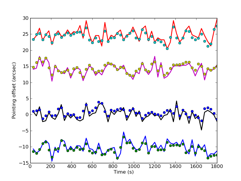
Figure 1: The solutions from the Pointing Selfcal algorithm using simulated data to verify the algorithm. The continuous lines show the pointing offsets as a function of time for four representative antennas while the filled-circles show the pointing offset solutions with 30 sec. solution interval.

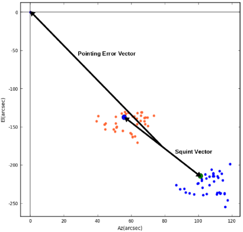
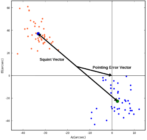
Figure 2: The results from the application of the Pointing SelfCal algorithm to the VLA data. Pointing error solutions along the elevation and azimuth axis for the R- and L-beams are shown with red and blue points. The average separation between these set of points corresponds to the polarization squint of the VLA antennas due to the off-axis feed location. The separation between the center of the squint vector and the origin corresponds to the antenna mechanical pointing error.

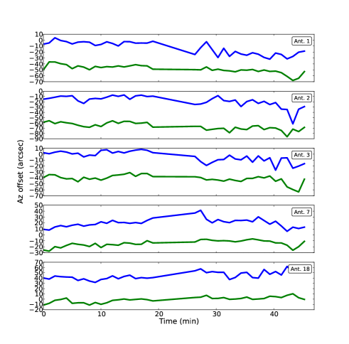
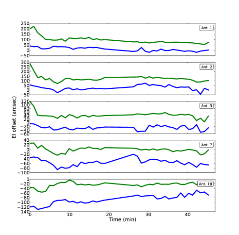
Figure 3: The pointing offsets in the antenna azimuth (left) and elevation (right) axises as a function of time for several antennas. The two curve in each panel correspond to the offsets for the R- and L-polarizations. The separation between the two curves in each panel correspond to the azimuth and elevation components of the polarization squint for each antenna.

4.2 Application to VLA data

To test the algorithm with real data, we used a wide-band observation of the IC2233 field with the VLA at L-Band. This data was imaged using about $\sim\!\!600$ MHz of bandwidth to generate the continuum sky model used as an input for the PSC algorithm. The VLA antenna optics creates an offset between the parallel-hand PBs (polarization squint) of $\sim\!\!6\%$ of the beam at any frequency, corresponding to $\sim\!\!110\arcsec$ at 1.5 GHz. To gain confidence in any antenna pointing offset that the solutions may show, we set up the PSC algorithm to solve for the offsets independently for both the polarizations (R and L). Difference in R- and L-solutions will then be a measure of the polarization squint and the mean value of these solutions ($[R_{offset}+L_{offset}]/2$) will be a measure of the antenna mechanical pointing error (which should be the same for both polarizations). In the antenna Az-El plane, the separation between the R and L solutions will then correspond to the length of the polarization squint vector, while a vector from the center of the squint vector to the origin of the Az-El plane would correspond to the actual antenna mechanical pointing error vector.

The results on the Az-El plane for two of the antennas in the array are shown in Fig. 2. The vector labeled “Squint Vector” shows the separation between the median values of the two offsets and is equal to $\sim\!\!120\arcsec$ and $105\arcsec$ for the two antennas. The vector labeled “Pointing Error Vector” from the center of the Squint Vector to the origin is a measure of the antenna mechanical pointing offsets, which has a magnitude of 3.5′and 0.5′ for these two antennas. These are large systematic pointing offsets, which were subsequently verified independently and corrected in the telescope software. As expected, after corrections, particularly for the first antenna, an improved antenna sensitivity was measured giving us a verification of the solutions and the sign convention used in the software.

The Az- and El-offsets of the RR and LL beams as a function of time from the nominal antenna pointing direction for a set of representative antennas with solution-intervals of 5 min and 600 MHz in time and frequency respectively are shown in Fig. 3. The PB model was derived using a geometric optics simulator for the antenna illumination patterns which includes the effects of aperture blockage, off-axis feed locations, and illumination taper (Brisken 2003). The rotation with PA and scaling of the PB with frequency was included in the model using the A-Projection algorithm. The sky brightness for this observation is dominated by two compact sources separated by $\sim\!\!25\arcsec$ with other weaker sources spread across the FoV. The scatter in the pointing solutions is due to three factors:

1. The actual sky brightness is dominated by two strong sources and so the constraints on the perpendicular directions are weak.

2. Imperfections in the sky model

3. The limitations of the PB model used, particularly as a function of frequency.

Analysis of independent holographic measurements (Perley 2016) show that in addition to systematic deviations from the expected value there are oscillations in the magnitude of the squint vector as a function of frequency due to standing waves in the antenna optics (Jagannathan et al. 2017), which were not included in the PB model. Some variations in the pointing offset solutions, including in the length of the squint vector could therefore be also real. The derived offsets as a function of time along the azimuth axis for a few antennas in the array are shown in Fig. 4. The solutions show significant differences in the antenna pointing errors between the antennas, as well as slow drifts over longer timescales ($\sim\!30~{}min$) – both of which are expected based on the regular pointing model measurements and anecdotal evidence from imaging results.

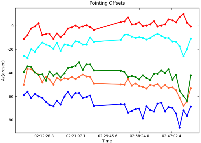
Figure 4: The solved antenna pointing offsets in the azimuth axis with time for a few representative antennas of the VLA.

4.3 Noise budget

In general, the stability and the error on the solved parameters depend directly on the SNR in the measured data (the RHS of Eq. 9) and on the number of free parameters. It is therefore important to devise algorithms that maximize data-SNR using as few free parameters as possible.

The equivalent thermal noise that contribute to the variance in the solution is reduced by a factor equal to the square root of the number of statistically independent samples averaged. The residuals in the PSC solver are averaged at each iteration across all baselines with a given antenna and for the duration of the solution intervals in time and frequency. Assuming that the pointing offsets at each antenna are statistically independent and random in nature, the noise contribution in the solver due to the thermal noise in the data is reduced by a factor equal to $\sqrt{\Delta\nu_{sol}\tau_{sol}\left(N_{ant}-1\right)}$ for solution intervals of $\Delta\nu_{sol}$ and $\tau_{sol}$ in frequency and time. On the other hand, the signal for the solver is the differential apparent-flux with respect to the pointing offsets in the FoV. Comparing this signal with the effective noise allows an estimate for the magnitude and the distribution of the sky brightness required for deriving pointing offset solutions. For a homogeneous array case with identical antennas, the SNR per parameter for an antenna-based pointing offsets solver is

$$SNR_{PSC}=\frac{\left|\nabla S\right|}{SEFD}~{}\sqrt{{\Delta\nu_{sol}\tau_{sol}}{\left(N_{ant}-1\right)}}$$ (16)

where

$$SEFD=\frac{2k_{b}T_{sys}}{(\eta_{A}\pi R^{2})}\times 10^{26}~{}(Jy)$$

$k_{b}$ is the Boltzmann’s constant. $R$, $\eta_{A}$ and $T_{sys}$ are the antenna aperture radius (in meters), efficiency and system temperature (in Kelvin) respectively. $\nabla S$ is the differential apparent integrated flux in the FoV with respect to the antenna pointing errors is given by:

$$\nabla S=\int\left(\frac{\partial{\mathsf{E}}}{\partial l}\otimes{\mathsf{E}^{*}}\right)~{}I^{M}(\vec{s})~{}d\vec{s}~{}~{}~{}~{}(Jy)$$ (17)

where ${\mathsf{E}}$ is the antenna far-field EFP and $I^{M}$ is a model for the sky brightness distribution as a function of the direction $\vec{s}$. For the VLA at L-band, $N_{ant}=27$ and $SEFD\approx\!358$ Jy ($T_{sys}=35$ K, $\eta_{A}=0.55$ and $R=12.5$ m). The total apparent flux in the VLA FoV at L-band above the thermal noise limit for a usable bandwidth of $800$ MHz and 1 min of integration in time is estimated to be few$\times 100$ mJy. In the absence of any other source of noise, solutions for antenna pointing offsets should be possible at reasonably high accuracy on very short timescales. Some numerical experiments suggest that reliable solutions are possible at several minutes timescale due to addition numerical noise, e.g. due to gridding, rotation of ${\mathsf{A}}^{M}$ with PA, inaccuracies in $I^{M}$ and ${\mathsf{A}}^{M}$, etc.

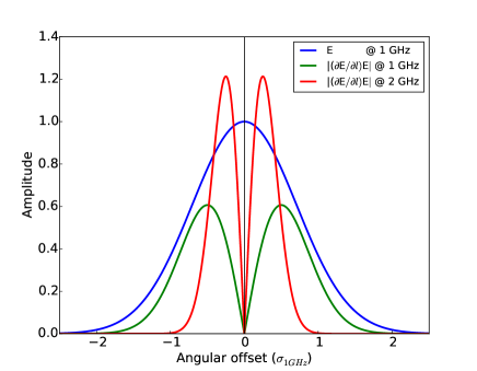
Figure 5: The curves show slices across the $\left|{\mathsf{E}(\nu)}\partial{\mathsf{E}(\nu)}/\partial l\right|$ function at the edges of a 1-GHz wide band (in green and red). The main-lobe of ${\mathsf{E}}$ at 1 GHz is approximated as a gaussian of width $\sigma_{1GHz}$ (in blue).

Analysis of Eq. 17 offers a few useful thumb-rules. The function $\left|\frac{\partial{\mathsf{E}}}{\partial l}\otimes{\mathsf{E}^{*}}\right|$ is a double-hump shaped curve with a null at the location of the peak of ${\mathsf{E}}$ (see Fig. 5). Therefore, while the sky brightness at the center of the PB does not contribute signal for the solver, the contribution of the flux around the center increases with the magnitude of the pointing error. This function peaks around the half-power-point of the PB. The flux in this region of the PB therefore contributes the maximum signal. The PSC algorithm therefore works well for fields where the sky brightness distribution is spread across the PB. This is almost always the case at low frequencies ($\lessapprox$few GHz) and for mosaic imaging which is typically the observing mode at high frequencies. Note that the antenna pointing errors also adversely affect imaging performance only for fields with significant flux away from the pointing center. The area under this curve is independent of frequency (changes in ${\partial{\mathsf{E}}}/{\partial l}$ and ${\mathsf{E}}$ compensates for each other as a function of frequency). Since the mechanical pointing errors are independent of frequency and on an average the low-frequency radio flux varies as $\nu^{-0.7}$, the signal for the pointing solver will increase with bandwidth, particularly at lower radio frequencies. More precise estimates for the SNR and solution timescales will require simulations using models for ${\mathsf{E}}$, the sky brightness and its spectral index distribution.

5 Discussions

5.1 Run-time performance analysis

The run-time cost of PSC has two components: computation of ${\mathsf{A}}_{ij}$ and $\nabla_{\!\!i}{\mathsf{A}}_{ij}$ and their application to $V_{ij}^{Obs}$ via A-Projection. Using Eqs. 14 and 15 with a precomputed ${\mathsf{A}}^{\circ}_{ij}$, the cost of evaluating ${\mathsf{A}}_{ij}$ and $\nabla_{\!i}{\mathsf{A}}_{ij}$ at each iteration becomes relatively insignificant and the total run-time cost is dominated by the cost of their application to $V_{ij}^{Obs}$. For a support size of $N_{sup}$ for ${\mathsf{A}}_{ij}$, this cost scales as $N_{vis}N^{2}_{sup}$, where $N_{vis}$ is the total number of data samples within the solution interval. Since the computations for each data sample is independent, this cost reduces linearly with parallelization by partitioning $N_{vis}$ across multiple computing cores. As a test case using a single CPU running at 1.2 GHz clock, each iteration of the PSC took about 1 sec per frequency channel for the VLA. Using all the 16 computing cores available, the run-time was reduced to $\sim 70$ millisec per channel, with the total run-time for convergence of $\sim 2$ min per solution.

Multi-threaded gridders (e.g., Golap (2015)) which can benefit from a much larger number of compute-cores available on massively parallel hardware like the modern GPUs may help in reducing the run-time cost by a large factor. For arrays that are non-coplanar for long-integration observations, the run-time cost of PSC increases with the W-term (Cornwell et al. 2008). However, for short solution interval the run-time cost may be largely independent of the W-term – by using the fact that arrays are instantaneously co-planar (Cornwell et al. 2012). However, more work is needed in these areas to determine the optimal computing architecture for PSC.

5.2 Use in real-time-calibration

Some modern-era radio telescopes assume that a Local Sky Model is available and use it to determine calibration parameters in real time without resorting to iteration over the model (see e.g. Tasse et al. (2012)). With some additional cost in computing, our algorithm for estimation of the pointing errors could be used to track any antenna pointing errors in real time and possibly correct the pointing errors in real-time.

5.3 Solving for PB shape

The PSC algorithm described above solves for the tip-tilt of the antenna by solving for a phase gradient across the antenna aperture. This does not however alter the Hermitian nature of an ideal aperture illumination pattern and therefore does not alter the predicted shape of the antenna PB. In practice, change in the shape of the antenna PB arises due to a variety of reasons including de-focus and astigmatism in the antenna optics, distortion of the main reflector with elevation, misplaced or misaligned elements in the antenna optics, and projection effects in aperture-array elements. Many of these terms result in a non-Hermitian aperture illumination pattern which, in addition to shape distortions also leads to complex-value PB. While pointing errors constitute the dominant direction-dependent error, errors due to the shape of the PB are also significant for the sensitivity offered by all modern radio telescopes. Its calibration is therefore also necessary.

The low-order A-Solver approach (Jagannathan et al. 2017) offers a method for a closed-loop Shape Selfcal (SSC) similar to the PSC algorithm. The A-Solver uses a physically motivated parametrized model of the antenna structure in a geometric optics (GO) simulator (Brisken 2003) for the antenna illumination pattern (AIP). Starting with reasonable values for these physical parameters, the A-Solver solves for these parameters by minimizing the difference between the predicted and holographically measured AIP. Since the model AIP needs to be predicted in the optimization iterations, it is important to use a simulator with a reasonably short run-time. Full-EM simulators are typically quite expensive (both, in capital and run-time costs). GO simulators on the other hand are less computationally complex and when used in the A-Solver, capture the dominant electromagnetic effects in the resulting optimized model. Jagannathan et al. (2017) show that this approach captures otherwise difficult to model effects like the effect of Standing Waves in the antenna optics and other higher order phase terms across the antenna aperture. These higher order phase terms severely affect the off-axis polarization leakage patterns and the A-Solver approach offers an effective method that can enable noise-limited full-Stokes imaging (not just Stoke-I imaging). The error analysis in Sec.4.3 above suggests that the use of a sky-model instead of the holographic measurements may be possible (from an SNR point of view) in the A-Solver for a closed-loop SSC algorithm. Note however that for many antenna arrays, shape changes are smooth and gradual and it may be sufficient to first derive the AIP model using holographic measurements and include the temporal evolution of the derived parameters separately. For the aperture-array elements, where these evolutions are more severe and faster, a closed-loop SSC may be required, and possible, using a model for the sky-brightness distribution (e.g. a pre-determined Global Sky Model).

6 Conclusions

In this paper we present the mathematical framework for calibration of direction-dependent effects (DDE) not known a priori. We also include a brief overview of the direction-independent (DI) calibration and the mathematical formulation of the existing DI SelfCal algorithm.

As an example of a DD calibration algorithm, we present the Pointing Selfcal (PSC) algorithm. As in DI SelfCal, given a model of the sky brightness distribution, the pointing offset vector per antenna is solved by iteratively minimizing the residual vector with respect to the antenna-based point offsets. We verified the PSC solver, first by applying it to simulated wide-band data for the VLA at L-band and show that the pointing offset vector is recovered correctly. We then also apply the PSC algorithm to on-sky data from the VLA at L-band. The VLA antenna optics has a polarization squint which results in an angular separation between the right- and left-circular polarization beams. To verify the PSC algorithm, the solver was set-up to solve for the pointing offset vector separately for the two polarizations. In the antenna Az-El plane, the difference between the pointing offset vectors for the two polarizations is a measure of the squint vector and the separation of the center of squint vector from the origin gives a measure of the mechanical antenna pointing offset. We verified that the PSC solver indeed recovers the average squint vector, though antenna-to-antenna variations were also large and significant. Some of the antennas had large mechanical pointing offsets, which were subsequently verified via independent measurement of the expected improvement in the antenna gain after correcting for them in the telescope software.

We also discuss the noise budget for the PSC algorithm. Analysis of the signal-to-noise ratio (SNR) available for the PSC solver as a function of the wide-band sky brightness distribution and telescope parameters leads to the following conclusions:

1. The PSC algorithm is optimal in utilizing the SNR due to the sky brightness distribution in the entire antenna field of view, rather than, for example, a few bright sources.

2. Antenna pointing offsets can be solved-for at high significance with the instantaneous sensitivity of most modern radio interferometric telescopes with wide-band receivers and typical sky brightness distributions.

3. While the sky brightness at the center of the PB does not contribute signal for the PSC solver, the contribution from around the center increases with the magnitude of the pointing offsets. This signal also peaks around the half-power points of the PB. The PSC algorithm therefore works well for observations where the sky brightness is distributed across the FoV. The degradation in the imaging performance due to the antenna pointing errors is also more significant for such observations. Emission spread across the FoV is typical at frequencies below a few GHz and at much higher frequencies where mosaic imaging of emission much larger than the antenna PB is often necessary.

4. We expect PSC to scale well in a parallel computing environment. Simple parallelization by data-partitioning is possible and efficient. Reduction in the run time by large factors using multi-threaded re-samplers (Golap 2015) deployed on massively parallel hardware remains a possibility, though more work is needed in this area to arrive at an optimal computing architecture.

5. The PSC is typically set-up for relatively short solution interval in time. For low-frequency observations, the increase in the run time due to the w-term may be mitigated by treating the array as co-planar for each solution interval (Cornwell et al. 2012).

The mathematical framework for DD calibration presented here can be extended for a Shape SelfCal (SSC) algorithm to account for the change in the shape of the aperture using the low-order A-Solver approach. In the A-Solver approach, the parameters describing the physical structure of the antenna are determined using a geometric optics predictor for the antenna aperture illumination pattern (AIP) and holographic measurements of the AIP (Jagannathan et al. 2017). Based on our estimate of the SNR typically available, it may be possible to develop an SSC algorithm using a model of the sky brightness distribution. More work is required, and in progress, in this area.

Finally, our algorithm could be used in the real-time calibration systems of modern-era radio telescopes where a Local Sky Model is assumed to be available. This will allow tracking of any antenna pointing errors in real time and possibly real-time corrections.

References

- Bhatnagar (1998) Bhatnagar, S. 1998, Computation Of Antenna Dependent Complex Gains, Tech. Rep. No. R00l72, National Centre for Radio Astrophysics, Pune. http://www.aoc.nrao.edu/~sbhatnag/GMRT_Offline/antsol/antsol.html
- Bhatnagar et al. (2004) Bhatnagar, S., Cornwell, T. J., & Golap, K. 2004, Solving for the antenna based pointing errors, Tech. rep., EVLA Memo 84. http://www.aoc.nrao.edu/vla/geninfo/memoseries/evlamemo84.ps
- Bhatnagar et al. (2008) Bhatnagar, S., Cornwell, T. J., Golap, K., & Uson, J. M. 2008, A&A, 487, 419. http://adsabs.harvard.edu/abs/2008A%26A...487..419B
- Bhatnagar et al. (2013) Bhatnagar, S., Rau, U., & Golap, K. 2013, The Astrophysical Journal, 770, 91. http://stacks.iop.org/0004-637X/770/i=2/a=91
- Brisken (2003) Brisken, W. 2003, Using Grasp8 To Study The VLA Beam, Tech. rep., EVLA Memo 58. "http://www.aoc.nrao.edu/vla/geninfo/memoseries/evlamemo58.ps"
- Cornwell et al. (2012) Cornwell, T., Voronkov, M., & Humphreys, B. 2012, Proc. SPIE 8500, Image Reconstruction from Incomplete Data VII: Wide field imaging for the Square Kilometre Array
- Cornwell (1999) Cornwell, T. J. 1999, in ASP Conf. Ser. 180: Synthesis Imaging in Radio Astronomy II, ed. G. B. Taylor, C. L. Carilli, & R. A. Perley. http://adsabs.harvard.edu/cgi-bin/nph-bib_query?bibcode=1999sira.conf.....T&db_key=AST
- Cornwell et al. (2008) Cornwell, T. J., Golap, K., & Bhatnagar, S. 2008, IEEE Journal of Selected Topics in Signal Processing, 2, 647
- Cornwell & Wilkinson (1981) Cornwell, T. J., & Wilkinson, P. N. 1981, MNRAS, 196, 1067. http://adsabs.harvard.edu/cgi-bin/nph-bib_query?bibcode=1981MNRAS.196.1067C&db_key=AST
- Golap (2015) Golap, K. 2015, Multi-threading gridders without copying and locks, Tech. rep., EVLA Memo 191. https://library.nrao.edu/public/memos/evla/EVLAM_191.pdf
- Hamaker et al. (1996) Hamaker, J. P., Bregman, J. D., & Sault, R. J. 1996, A&AS, 117, 137. http://adsabs.harvard.edu/cgi-bin/nph-bib_query?bibcode=1996A%26AS..117..137H&db_key=AST
- Jagannathan et al. (2017) Jagannathan, P., Bhatnagar, S., Brisken, W., & Taylor, A. R. 2017, The Astrophysical Journal (submitted)
- Jones (1941) Jones, R. C. 1941, J. Opt. Soc. America, 31, 488
- Mueller (1948) Mueller, H. 1948, J. Opt. Soc. America, 38, 661
- Perley (2016) Perley, R. 2016, Jansky Very Large Array Primary Beam Characteristics, Tech. rep., EVLA Memo 195. "https://library.nrao.edu/public/memos/evla/EVLAM_195.pdf"
- Perley et al. (2011) Perley, R. A., Chandler, C. J., Butler, B. J., & Wrobel, J. M. 2011, The Astrophysical Journal Letters, 739, L1. http://stacks.iop.org/2041-8205/739/i=1/a=L1
- Press et al. (1992) Press, W., Teukolsky, S., Vetterling, W., & Flannery, B. 1992, Numerical Recipes in C (Cambridge: Cambridge University Press)
- Rau & Cornwell (2011) Rau, U., & Cornwell, T. J. 2011, A&A, 532, 17. http://stacks.iop.org/0004-637X/770/i=2/a=91
- Tasse et al. (2012) Tasse, C., van Diepen, G., van der Tol, S., et al. 2012, Comptes Rendus Physique, 13, 28
- Thompson & Daddario (1982) Thompson, A. R., & Daddario, L. R. 1982, Radio Science, 17, 357. http://adsabs.harvard.edu/cgi-bin/nph-bib_query?bibcode=1982RaSc...17..357T&db_key=AST
- Thompson et al. (2017) Thompson, A. R., Moran, J. M., & Swenson, G. W., J. 2017, Interferometry and Synthesis in Radio Astronomy (John Wiley & Sons, Inc.)