NuGrid Stellar Data Set. II. Stellar Yields from H to Bi for Stellar Models with $M_{\rm ZAMS}=1$ to $25\,{\rm M}_{\odot}$ and $Z=0.0001$ to $0.02$

Abstract

We provide here a significant extension of the NuGrid Set 1 models in mass coverage and toward lower metallicity, adopting the same physics assumptions. The combined data set now includes the initial masses $M_{\rm ZAMS}/\,{\rm M}_{\odot}$ = 1, 1.65, 2, 3, 4, 5, 6, 7, 12, 15, 20, 25 for $Z=0.02,0.01,0.006,0.001,0.0001$ with $\alpha$-enhanced composition for the lowest three metallicities. These models are computed with the MESA stellar evolution code and are evolved up to the AGB, the white dwarf stage, or until core collapse. The nucleosynthesis was calculated for all isotopes in post-processing with the NuGrid mppnp code. Explosive nucleosynthesis is based on semi-analytic 1D shock models. Metallicity-dependent mass loss, convective boundary mixing in low- and intermediate mass models and H and He core burning massive star models is included. Convective O-C shell mergers in some stellar models lead to the strong production of odd-Z elements P, Cl, K and Sc. In AGB models with hot dredge-up the convective boundary mixing efficiency is reduced to accommodate for its energetic feedback. In both low-mass and massive star models at the lowest metallicity H-ingestion events are observed and lead to i-process nucleosynthesis and substantial ${}^{\makebox[7.0pt][r]{$\scriptstyle 15$}}_{\makebox[7.0pt][r]{$\scriptstyle$}}\mathrm{N}$ production. Complete yield data tables, derived data products and online analytic data access are provided.

1 Introduction

Stellar yields data are a fundamental input for galactic chemical evolution models (e.g. Romano et al., 2010; Nomoto et al., 2013; Mollá et al., 2015), hydrodynamic models (e.g. Scannapieco et al., 2005) and chemodynamic models (e.g. Few et al., 2012; Côté et al., 2013; Schaye et al., 2015). Gibson (2002) and Romano et al. (2010) showed that results of chemical evolution models are strongly affected by uncertainties related to the choice of the yield set: for example, yield sets lead to $0.6\,\mathrm{dex}$ differences in [C/O] ratio and $0.8\,\mathrm{dex}$ for [C/Fe] in their galaxy models. These yield studies couple separate yield sets for massive and low-mass stars. These two separate sets often use different stellar evolution codes and different nuclear networks. In this paper, we present yields based on stellar models of a range of initial masses and metallicities calculated with the MESA (Paxton et al., 2011) stellar evolution code and post-processed with the NuGrid post-processing network (Pignatari et al., 2016b, P16).

This work builds upon the study by P16, and includes important improvements over this study. In this work, the same stellar code MESA (Paxton et al., 2011) is used for the full stellar set, while the yields set from P16 are calculated with different stellar evolution codes: MESA for AGB star models and the Geneva stellar evolution code (Eggenberger et al., 2008, GENEC) for massive star models. In this work, we have extended the set of models by adding more low-mass, intermediate-mass and massive stars: we provide models also for $M_{\rm ZAMS}=1\,{\rm M}_{\odot}$, $6\,{\rm M}_{\odot}$, $7\,{\rm M}_{\odot}$ and $12\,{\rm M}_{\odot}$ stars, including now low-mass supernova progenitors and super-AGB models, not included in the P16 set. In particular, a finer grid for intermediate-mass stars is important for galactic chemical evolution applications of the yield set, since these stars are important producers of ${}^{\makebox[7.0pt][r]{$\scriptstyle 13$}}_{\makebox[7.0pt][r]{$\scriptstyle$}}\mathrm{C}$ and ${}^{\makebox[7.0pt][r]{$\scriptstyle 14$}}_{\makebox[7.0pt][r]{$\scriptstyle$}}\mathrm{N}$, in particular at low metallicity (e.g. Siess, 2010; Ventura & D’Antona, 2011; Karakas et al., 2012; Ventura et al., 2013; Gil-Pons et al., 2013; Doherty et al., 2014). Models in the narrow transition mass range from AGB stars to massive stars that may including electron-capture SN (Gutierrez et al., 1996; Jones et al., 2013, 2014), as well as yields for Type Ia SN are beyond the scope of this work. Finally, in addition to new masses the yield set is extended by adding models with three lower metallicities for all initial masses. Below $Z=0.01$ an $\alpha$-enhanced initial abundance is adopted which leads to [Fe/H] = -1.24, -2.03 and -3.03 for $Z=0.006,0.001$ and $Z=0.0001$.

The yields of massive AGB stars and super-AGB (S-AGB) stars depend on the nucleosynthesis during hot-bottom burning (HBB, Sackmann & Boothroyd, 1992; Lattanzio et al., 1996; Doherty et al., 2010; García-Hernández et al., 2013; Ventura et al., 2015). There are two options to resolve HBB in stellar models: either to couple the mixing and burning operators or choose time steps smaller than the convective turnover timescale $\tau_{\rm conv}$ of the envelope (e.g. $\tau_{\rm conv}\sim\mathrm{hrs}$ for the $M_{\rm ZAMS}=4\,{\rm M}_{\odot}$, $Z=0.0001$ model). The difficulty in modeling the HBB process is that the large networks required for the heavy element nucleosynthesis in HBB require considerable computing time. But post-processing codes which decouple mixing and burning operators need to resolve the extremely short mixing time scale when HBB convective-reactive conditions are relevant. In this work we present a nested-network post-processing approach in which mixing and burning operators are coupled. With this approach we accurately calculate stellar yields also for isotopes affected by HBB conditions.

Ingestion events are common at low and zero-metallicity in AGB models of low mass (e.g. Fujimoto et al., 2000; Cristallo et al., 2009), in He-core flash in low-metallicity low-mass models (e.g. Campbell et al., 2010), and in S-AGB models in a wide range of metallicities (e.g. Gil-Pons & Doherty, 2010; Jones et al., 2016). The energy release as well as nuclear burning on the convective turn-over time scale due to H ingestion might violate the treatment of convection via mixing-length theory (MLT) (Herwig, 2001b) and/or the assumption of hydrostatic equilibrium (e.g. in S-AGB models Jones et al., 2016). The three-dimensional (3D) hydrodynamic simulations of H ingestion of the post-AGB star Sakurai’s object show that global and non-radial instabilities can be triggered in such convective-reactive phases can not be simulated in 1D stellar evolution (Herwig et al., 2014). Herwig et al. (2011) and Herwig (2001b) also reported that observational abundances and light curve of Sakurai’s object can not be explained with 1D models based on the MLT. Thus, the predictive power of 1D stellar evolution models to describe H ingestion events might be limited. The models nevertheless provide information about the frequency of such events as well as their potential impact on the production of elements.

Yield tables are typically provided in the literature but in order to trace back the underlying reasons for certain abundance features in yield tables it is important to have access to the full stellar models. In this paper we provide full web access of the stellar evolution and post-processing data including yield tables and an interactive interface to analyze and retrieve data.

The paper is organized as follows: in Sect. 2 we describe the methods used to perform the stellar evolution simulations, the semi-analytic models of the core-collapse supernova (CCSN) shock and post-processing. In Sect. 3 we introduce the general properties of stellar models and features related to low metallicity. In Sect. 4 we analyze the final yields at low metallicity. The latter are grouped by nucleosynthesis process. We discuss our assumptions in Sect. 5 and compare the results with available literature. In Sect. 6 we summarize the results.

2 Methods

The yields presented in this paper have been produced using 1D stellar evolution calculations and a semi-analytic prescription for CCSN shock propagation together with a post-processing nuclear reaction network. The details of three steps are described in this section.

2.1 Stellar evolution

The stellar evolution calculations were performed using the MESA stellar evolution code (Paxton et al., 2011), rev. 3709. The AGB models in NuGrid Set 1 (Pignatari et al., 2016b) were not recomputed, and those models used rev. 3372 of MESA. The AGB models in this work adopt the same opacities as P16, in which case the two revisions produce similar results. For example, the time-evolution of H-free core masses agree to within $0.2\,\%$. A comparison of AGB models of newer MESA revisions with the P16 models is presented in Battino et al. (2016). MESA rev. 3709 was also used for the massive star models. This is in contrast with P16, who used GENEC (Eggenberger et al., 2008). A detailed comparison of GENEC and MESA (and KEPLER) massive star models at solar metallicity was performed by Jones et al. (2015), who found that the CO core masses are within $10\,\%$ to $15\,\%$ of one another and the elemental abundances produced in the He core by the weak s-process agree within 30 %. The physics assumptions up to the end of core He burning in the massive star models are as in Jones et al. (2015).

2.1.1 Initial composition and nuclear reaction network

We use solar-scaled initial abundance at $Z=0.02$ and $Z=0.01$ as in P16, based on Grevesse & Noels (1993) and with the isotopic ratios from Lodders (2003). At $Z=0.006$ and below we enhance the $\alpha$ isotopes ${}^{\makebox[7.0pt][r]{$\scriptstyle 12$}}_{\makebox[7.0pt][r]{$\scriptstyle$}}\mathrm{C}$, ${}^{\makebox[7.0pt][r]{$\scriptstyle 16$}}_{\makebox[7.0pt][r]{$\scriptstyle$}}\mathrm{O}$, ${}^{\makebox[7.0pt][r]{$\scriptstyle 20$}}_{\makebox[7.0pt][r]{$\scriptstyle$}}\mathrm{Ne}$, ${}^{\makebox[7.0pt][r]{$\scriptstyle 24$}}_{\makebox[7.0pt][r]{$\scriptstyle$}}\mathrm{Mg}$, ${}^{\makebox[7.0pt][r]{$\scriptstyle 28$}}_{\makebox[7.0pt][r]{$\scriptstyle$}}\mathrm{Si}$, ${}^{\makebox[7.0pt][r]{$\scriptstyle 32$}}_{\makebox[7.0pt][r]{$\scriptstyle$}}\mathrm{S}$, ${}^{\makebox[7.0pt][r]{$\scriptstyle 36$}}_{\makebox[7.0pt][r]{$\scriptstyle$}}\mathrm{Ar}$, ${}^{\makebox[7.0pt][r]{$\scriptstyle 40$}}_{\makebox[7.0pt][r]{$\scriptstyle$}}\mathrm{Ca}$ and ${}^{\makebox[7.0pt][r]{$\scriptstyle 48$}}_{\makebox[7.0pt][r]{$\scriptstyle$}}\mathrm{Ti}$. The $\alpha$ enhancements were derived from fits of halo and disk stars from Reddy et al. (2006) and references therein. For each enhanced isotope ${\alpha}$ we apply Eq. 1 where $A_{\alpha}$ and $B_{\alpha}$ were derived from the fits for metallicities $-1\leq[\mathrm{Fe/H}]\leq 0$ (Reddy et al., 2006). For $[\mathrm{Fe/H}]<-1$ we assume a constant $[X_{\alpha}/\mathrm{Fe}]$ of $[X_{\alpha}/\mathrm{Fe}]=-A_{\alpha}+B_{\alpha}$.

$$[X_{\alpha}/\mathrm{Fe}]=A_{\alpha}[\mathrm{Fe/H}]+B_{\alpha}$$ (1)

For isotopes of Ne, S and Ar values from Kobayashi et al. (2006) were adopted. The resulting $[X_{\alpha}/\mathrm{Fe}]$ and mass fractions for $Z=0.0001$ are shown in Table 1. The fit result gives $\mathrm{[O/Fe]}=0.89$ which is close to the top of the [O/Fe] distribution but within the maximum given in Reddy et al. (2006). For the initial abundance of Li in AGB models with $M_{\rm ZAMS}>3\,{\rm M}_{\odot}$ we choose as a lower limit the Li plateau (Sbordone et al., 2010). In other stellar models the initial Li abundance was unintentionally scaled down with metallicity as other light elements and unrealistic values were adopted. An overview of the model assumptions is presented in the following sections, and a comparison with P16 is given in Table 2.

In the low-mass stellar models up to $M_{\rm ZAMS}=3\,{\rm M}_{\odot}$ we use the same network in MESA as in P16 (agb.net). For the massive AGB and super-AGB models ($4\,{\rm M}_{\odot}\leq M_{\rm ZAMS}\leq 7\,{\rm M}_{\odot}$) we use the network agbtomassive.net which includes an extended network for C, O and Ne burning and relevant electron-capture reactions. No significant rate updates have been adopted compared to P16. The nuclear reaction network for stellar models with masses $M_{\mathrm{zams}}\geq 12\,{\rm M}_{\odot}$ is the same as in Jones et al. (2015, their Table 2) from the pre-main sequence until the depletion of oxygen in the core, at which point the network is reduced to approx21.net to follow Si burning and deleptonisation in the Fe core.

2.1.2 Mass loss

Semi-empirical prescriptions for mass loss (e.g. Vassiliadis & Wood, 1993; van Loon et al., 2005) are still commonly used in stellar evolution. In order to stay consistent with P16 we apply the mass loss prescription by Reimers (1975) for the red giant branch phase and the prescription of Blöcker & Schönberner (1995) for the AGB phase. Both prescription are functions of the mass, luminosity and radius of the stellar model. The efficiency parameter $\eta_{\rm Bloecker}$ is increased to mimic the effect of the C-rich dust-driven phase as described in P16. A more realistic hydrodynamic approach to mass loss models (e.g. Mattsson et al., 2010) in combination with observational calibrations taking into account better data now available (e.g. Rosenfield et al., 2014) should ultimately be deployed for yield calculations.

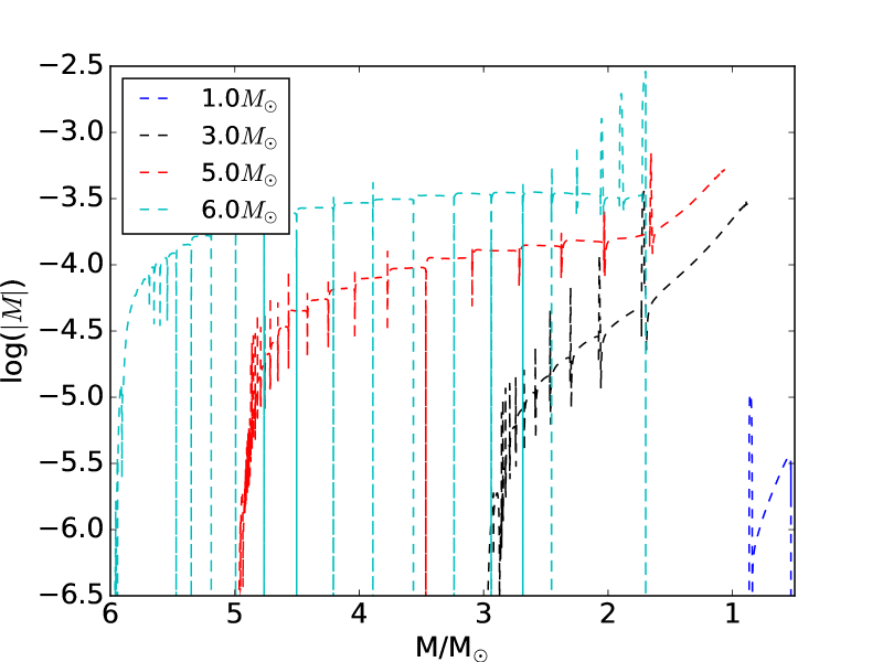
Figure 1: 3D spline fit of $\eta_{\rm Bloecker}$ dependent of mass and metallicity based on Herwig (2004a) and P16 (top). The green circles represent additional ad-hoc values. Mass loss in $\,{\rm M}_{\odot}/{\rm yr}$ for stars of $Z=0.0001$ based on the mass-metallicity fits of $\eta_{Bloecker}$ (bottom).

Our approach here aims to bridge the mass loss choice of P16 with that of Herwig (2004a, H04) who adopted a metallicity dependent mass loss based on van Loon (2000). Since the H04 and these $Z=0.0001$ MESA models are slightly different we derive values of $\eta_{\rm Bloecker}$ to be used in the MESA models to obtain the same mass loss as in H04. We then fit $\eta_{\rm Bloecker}$ in the mass-metallicity plane to be constrained by the mass loss adopted in P16 for $Z=0.02$ and $0.01$ and by H04 for $Z=0.0001$. The resulting spline fit of $\eta_{\rm Bloecker}$ in the mass-metallicity plane is shown in Fig. 1. We have added ad-hoc values for stellar models of $M_{\rm ZAMS}/\,{\rm M}_{\odot}$ = 4, 6, 7, 8 for solar and half-solar metallicity to extrapolate the general trend of decreasing $\eta_{\rm Bloecker}$ at higher initial mass. The fit corresponds to the general notion that $\eta_{\rm Bloecker}$, and with it the mass loss, decreases for low-mass AGB stars with decreasing metallicity (Willson, 2000). This contrasts with the observational findings of shorter AGB lifetimes with lower metallicity in low-mass AGB stars (Rosenfield et al., 2014).

The mass loss prescription adopted in the massive star models depends on the effective temperature $T_{\rm eff}$ and the surface hydrogen mass fraction X(H) as in Glebbeek et al. (2009). For $T_{\rm eff}\geq 1.1\times 10^{4}\,\mathrm{K}$ and $X({\rm H})\geq 0.4$ we adopt the mass loss rate of Vink et al. (2001). At lower temperatures the Vink et al. (2001) rate transits into the de Jager et al. (1988) rate and the latter is adopted below $T_{\rm eff}=10^{4}\,\mathrm{K}$. If $X({\rm H})<0.4$ we adopt either Nugis & Lamers (2000) when $T_{\rm eff}<10^{4}\,\mathrm{K}$, otherwise de Jager et al. (1988). The Nugis & Lamers (2000) and Vink et al. (2001) rates depend explicitly on metallicity. See Glebbeek et al. (2009) for further details. A correction factor of 0.8 is adopted for mass loss rates of massive star models as deduced for MS OB stars in Maeder & Meynet (2001).

2.1.3 Hot-bottom burning

HBB is the activation of the CNO cycle at the bottom of the convective envelope in massive AGB and S-AGB stars (Scalo et al., 1975; Sackmann & Boothroyd, 1992). Higher temperatures in the AGB envelopes at lower metallicity lead to the activation of HBB at lower initial mass compared to AGB models of higher metallicity. This increases the number of stars which experience HBB with decreasing metallicity.

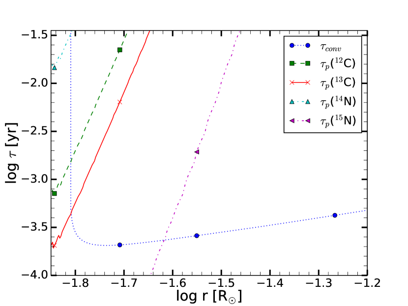
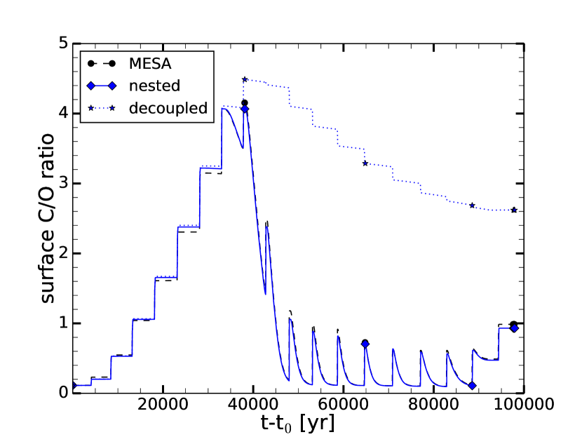
Figure 2: Convective turnover timescale $\tau_{\rm conv}$ and CNO reaction timescales $\tau_{p}$ relevant for HBB at the bottom of the convective envelope of the $M_{\rm ZAMS}=4\,{\rm M}_{\odot}$, $Z=0.0001$ model (top). The evolution of the surface C/O number ratio of this stellar model based on the coupled solution of MESA, on the nested-network method and the decoupled method (middle). $t_{0}$ marks the beginning of the TP-AGB phase. Surface CNO abundances from the nested-network method in comparison with abundances from MESA (bottom).

During HBB the mixing timescale of the convective envelope $\tau_{\rm conv}$ and nuclear timescales of CNO p-capture reactions $\tau_{p}$ become similar as shown for the $M_{\rm ZAMS}=4\,{\rm M}_{\odot}$, $Z=0.0001$ model in Fig. 2. $\tau_{\rm conv}$ is calculated as $\tau_{\rm conv}=l_{\rm MLT}^{2}/D$ where $D$ is the diffusion coefficient and $l_{\rm MLT}$ is the mixing length according to MLT. The coupling of mixing and burning operators in stellar evolution codes allow to resolve HBB correctly. Typically, post-processing codes decouple mixing and burning in order to solve differential equations for large reaction networks including heavy elements. To model HBB in the decoupled approach it is necessary to resolve the mixing timescale at the bottom of the convective envelope. This is just hours, for example in this $M_{\rm ZAMS}=4\,{\rm M}_{\odot}$, $Z=0.0001$ model (Fig. 2), which is short compared to the interpulse phases of tens of thousands of years. Cristallo et al. (2015) calculate heavy elements with a large network in their stellar evolution code and approximate CNO production due to HBB with a burn-mix-burn step. Our solution is to solve the coupled reaction and diffusion equations for a subset of important isotopes (see Sect. 2.3).

2.1.4 Convective boundary mixing treatment

We apply convective boundary mixing (CBM) at all convective boundaries of the AGB models. CBM is modeled with an exponential-diffusive convective boundary mixing model (Freytag et al., 1996; Herwig, 2000). A CBM efficiency of $f=0.014$ is used at all convective boundaries of AGB models except for the bottom of the pulse-driven convective zone (PDCZ) and during the third dredge-up (TDUP) of the thermal-pulse (TP)-AGB stage. Motivated by 2D and 3D simulations of Herwig et al. (2007) a lower CBM efficiency of $f_{\rm PDCZ}=0.008$ is applied at the PDCZ bottom boundary. An increased mixing efficiency of $f_{\rm CE}=0.126$ is applied at the bottom of the convective envelope during the TDUP which is calibrated for low-mass stellar models to produce the ${}^{13}\mathrm{C}$ pocket (Herwig et al., 2003). This approach is the same as in P16.

CBM is only accounted for in the massive star models from the pre-main sequence up to the end of core He burning. It is implemented as the exponential diffusion model of Freytag et al. (1996) with $f=0.022$ at all convective boundaries except for the bottom of convective shells in which nuclear fuel is burning, where $f=0.005$ was used. From the extinction of core He burning, which we have defined as the time when the central mass fraction of helium falls below $10^{-5}$, $f$ is set to zero, equivalent to assuming no CBM.

Corrosive H-burning during TDUP in low-metallicity massive AGB stars leads to an increase of the TDUP efficiency and is referred to as hot dredge-up (HDUP, Herwig, 2004a). The application of CBM at the bottom of the convective envelope results in strong burning of the mixed protons below the envelope and extreme TDUP efficiencies in these massive AGB models at low metallicity. In a $M_{\rm ZAMS}=5\,{\rm M}_{\odot}$, $Z=0.0001$ test model with CBM parameter $f_{\rm CE}=0.126$ used for the ${}^{13}\mathrm{C}$-pocket formation in low-mass AGB stars the TDUP penetrates into the C/O core after the sixth TP as shown in the Kippenhahn diagram in Fig. 3. This finding is in agreement with Herwig (2004b) who found that the HDUP can penetrate into the C/O core and terminate the AGB phase (see also Goriely & Siess, 2004). The abundance profile during the TDUP at the bottom of the convective envelope shows the peak of nuclear burning in the CBM region which steepens the radiative gradient and hence leads to a deeper penetration of the envelope into the He intershell (Fig. 3). Karakas (2010) models do not experience HDUP because the authors do not model CBM in the stellar evolution simulation. Instead, they introduce an ad-hoc partial mixing zone for the formation of the ${}^{13}\mathrm{C}$-pocket in the post-processing simulations.

One way to reduce the vigour of H burning during the HDUP is the reduction of $f_{\rm CE}$. The efficiency of CBM at the lower boundary of the convective envelope in massive and S-AGB is not known. Investigations of the impact of CBM efficiency on structure and nucleosynthesis such as for S-AGB models by Jones et al. (2016) are required. A physical interpretation of the assumption of a reduced CBM is based on the buoyancy of the mixed and burning material which hinders boundary mixing. The situation is similar to the bottom of convective burning shells in the late stage of massive stars where the energy release leads to a lower CBM and a stiffer boundary (e.g. Cristini et al., 2016; Jones et al., 2017). Following Herwig (2004a), we limit CBM by reducing $f_{\rm CE}$ here to $0.01$ for $M_{\rm ZAMS}\geq 4\,{\rm M}_{\odot}$ models if the dredge-up after a thermal pulse is hot (Table 3). With this approach we prevent the termination of the AGB phase due to too extreme H burning during the TDUP. The limiting of $f_{\rm CE}$ in massive and S-AGB models is new in this work, compared to P16. Other choices of CBM efficiencies are as in P16 (Table 2).

2.2 Semi-analytic CCSN explosions

We use a semi-analytic approach for core-collapse supernova explosions as described in P16. The method drives a shock off the proto-neutron star based on a mass cut derived from Fryer et al. (2012, F12). The mass cuts are mass- and metallicity dependent and are provided for delayed and a rapid explosion prescription. The mass coordinates based on these models are shown in Table 4. For some massive star models such as the $M_{\rm ZAMS}=15\,{\rm M}_{\odot}$, $Z=0.006$ model the mass cut is deeper located than than the outer edge of the Fe core as visible from the Fe-core masses in Table 5.

One of the big uncertainties in the yields is the position of the mass cut. The data from F12 were based on fits to the stellar structures produced by comparing the models from a range of stellar evolution codes (Woosley et al., 2002; Limongi & Chieffi, 2006; Young et al., 2009). These mass-cut prescriptions were then validated against the compact remnant mass distribution (Belczynski et al., 2012). For these stellar evolution models, the mass cut is fairly similar for models with $M_{\rm ZAMS}<25\,{\rm M}_{\odot}$. However, in particular for the $M_{\rm ZAMS}=12\,{\rm M}_{\odot}$ model, the core from the MESA model is much larger than that produced by the Kepler code. This corresponds to much higher densities in the inner $2\,{\rm M}_{\odot}$ and, based on the F12 results, we expect the MESA $M_{\rm ZAMS}=12\,{\rm M}_{\odot}$ models to collapse down to a black hole rather than explode to produce a low-mass neutron star. In this case, the $M_{\rm ZAMS}=12\,{\rm M}_{\odot}$ stars would not provide SN yields and would contribute to the chemical evolution of the Galaxy only by stellar winds. In part, these results for the $12\,{\rm M}_{\odot}$ stellar progenitors are caused by the use of a small nuclear network in the MESA code during Si burning.

At earlier times, the MESA models with $M_{\rm ZAMS}=12\,{\rm M}_{\odot}$ and GENEC models with $M_{\rm ZAMS}=15\,{\rm M}_{\odot}$ of P16 are very similar. Therefore, for the MESA models with $M_{\rm ZAMS}=12\,{\rm M}_{\odot}$ we also use the mass cut prescription of F12 under the assumption of $M_{\rm ZAMS}=15\,{\rm M}_{\odot}$ as adopted for these GENEC models. This allows to provide a SN yield set of these MESA models at all metallicities. For more massive MESA models, we use the mass cut prescription of F12 as in P16. The same semi-analytic CCSN prescription as in P16 is applied, except the modification of the $M_{\rm ZAMS}=12\,{\rm M}_{\odot}$ models.

2.3 Nucleosynthesis code and processed data

The temperature, density and diffusion coefficient (from the mixing length theory of convection along with the convective boundary mixing model) $T(m),~{}\rho(m)$ and $D(m)$ in the MESA stellar evolution models are saved every time step and post-processed with the multi-zone NuGrid code mppnp using and the same reaction network as in P16. To summarize: every stellar evolution time step, the 1097-isotope nuclear reaction network is solved using a first-order Newton-Raphson backward Euler integration, which is followed by an implicit diffusion solve. The network adapts the problem size every time step (and every computational grid cell) depending upon the reaction flux of each isotope at current state. The AGB models of P16 were not post-processed again, but are part of the updated analysis presented here.

In Sect. 2.1.3 we described issues that arise with such an operator-splitting method during hot bottom burning in models of massive AGB and super-AGB stars. To predict realistic abundances in these conditions we have implemented a nested-network method to solve the coupled mixing and burning equations for a small network which includes species which are affected by HBB. We solve the small network for zones of the convective envelope and a large decoupled network for the whole stellar model. After each time step the abundances from the coupled solution replace the abundances from the large network. The coupled solution is merged into the large network by normalizing the total abundance of isotopes of the small network to be equal to the total abundance of the corresponding isotopes of the large network. Here, the coupled solution includes mixing and burning, and as in all of the post-processing the structure is provided by MESA. Just as a reminder, MESA solves structure, mixing and burning operators together. The small network models the Cameron-Fowler transport mechanism and ${}^{\makebox[3.5pt][r]{$\scriptstyle 7$}}_{\makebox[3.5pt][r]{$\scriptstyle$}}\mathrm{Li}$ production (Cameron & Fowler, 1971), CNO, NeNa and MgAl cycles and includes isotopes up to ${}^{\makebox[7.0pt][r]{$\scriptstyle 35$}}_{\makebox[7.0pt][r]{$\scriptstyle$}}\mathrm{Cl}$ similar to Siess (2010). Heavier isotopes, which are only included in the large network, do not take part in HBB nucleosynthesis according to the present state-of-the-art (e.g. review by Herwig, 2005). As such we don’t expect the heavier isotopes to be affected by our choice of decoupling of burning and mixing.

We compare of the surface C/O ratio of the $M_{\rm ZAMS}=4\,{\rm M}_{\odot}$, $Z=0.0001$ model of the coupled solution with the nested-network solution and the decoupled solution (Fig. 2). Our nested-network method results in the same evolution of the surface C/O ratio. The decoupled solution based time steps as given for the coupled solution of MESA strongly overestimates the surface C/O ratio compared to the coupled solution from MESA. We find good agreement of the surface abundance of CNO isotopes based on our nested-network method in comparison with predictions from MESA (Fig. 2).

The final stellar yields of CNO isotopes based on the nested-network method are similar to Herwig (2004a, H04) and Karakas (2010, K10) who couple mixing and burning (Table 6). Neither study includes s-process species, although more recent work by Karakas & Lugaro (2016) for $0.007<Z<0.03$ does now include heavy elements. The high ${}^{\makebox[7.0pt][r]{$\scriptstyle 12$}}_{\makebox[7.0pt][r]{$\scriptstyle$}}\mathrm{C}$/${}^{\makebox[7.0pt][r]{$\scriptstyle 13$}}_{\makebox[7.0pt][r]{$\scriptstyle$}}\mathrm{C}$ ratio of the decoupled solution shows that HBB is not properly resolved. Even larger values of Cristallo et al. (2015, C15) could be due to resolution issues during HBB with the mix-burn-mix approximation. The nested-network approach predicts Li production via HBB as well because Cameron-Fowler mechanism is resolved. In summary, the nested-network method allows to predict Li, CNO isotopes and heavy elements in these HBB stellar models.

The total stellar yield of element/isotope $i$ of a stellar model with initial mass $m$ includes the yield from stellar winds and the SN explosion as in P16. The yield ejected by stellar winds ${\rm EM}^{\rm wind}_{\rm im}$ is calculated as

$${\rm EM}^{\rm wind}_{\rm im}=\int^{\tau(m)}_{0}\dot{M}(m,t)\,X^{S}_{i}(m,t)dt$$ (2)

where $\dot{M}(m,t)$ is the mass loss rate, $X^{S}_{i}(m,t)$ is the mass fraction of the element/isotope $i$ at the surface and $\tau(m)$ is the stellar lifetime. The yield from the SN ejecta ${\rm EM}^{\rm SN}_{im}$ is derived as

$${\rm EM}^{\rm SN}_{\rm im}=\int^{m_{\tau}}_{M_{{\rm rem},m}}\,X_{i}(m_{r})dm_{r}$$ (3)

where $X_{i}(m_{r})$ is the mass fraction of element/isotope $i$ at mass coordinate $m_{r}$ and $M_{{\rm rem},m}$ is the remnant mass. Pre-SN yields are calculated as ${\rm EM}^{\rm SN}_{\rm im}$ but without taking into account the nucleosynthesis from the SN shock. Instead, the ejecta of matter at the point of collapse is considered. The overproduction factor $OP_{\rm im}$ of element/isotope $i$ of the stellar model with initial mass $m$ is calculated as

$${\rm OP}_{\rm im}=\frac{{\rm EM}_{\rm im}}{X_{i}^{0}M_{\rm ej}}$$ (4)

where ${\rm EM}_{\rm im}$ and $X_{i}^{0}$ is the total ejected mass and initial mass fraction of element/isotope $i$ respectively. $M_{\rm ej}$ is the total ejected mass.

Isotope	[$X_{i}$/Fe]	$X_{i}$
${}^{\makebox[7.0pt][r]{$\scriptstyle 12$}}_{\makebox[7.0pt][r]{$\scriptstyle$}}\mathrm{C}$	0.562	1.25E-05
${}^{\makebox[7.0pt][r]{$\scriptstyle 16$}}_{\makebox[7.0pt][r]{$\scriptstyle$}}\mathrm{O}$	0.886	7.41E-05
${}^{\makebox[7.0pt][r]{$\scriptstyle 20$}}_{\makebox[7.0pt][r]{$\scriptstyle$}}\mathrm{Ne}$	0.5	5.75E-06
${}^{\makebox[7.0pt][r]{$\scriptstyle 24$}}_{\makebox[7.0pt][r]{$\scriptstyle$}}\mathrm{Mg}$	0.411	1.51E-06
${}^{\makebox[7.0pt][r]{$\scriptstyle 28$}}_{\makebox[7.0pt][r]{$\scriptstyle$}}\mathrm{Si}$	0.307	1.51E-06
${}^{\makebox[7.0pt][r]{$\scriptstyle 32$}}_{\makebox[7.0pt][r]{$\scriptstyle$}}\mathrm{S}$	0.435	1.09E-05
${}^{\makebox[7.0pt][r]{$\scriptstyle 36$}}_{\makebox[7.0pt][r]{$\scriptstyle$}}\mathrm{Ar}$	0.3	1.64E-07
${}^{\makebox[7.0pt][r]{$\scriptstyle 40$}}_{\makebox[7.0pt][r]{$\scriptstyle$}}\mathrm{Ca}$	0.222	1.21E-07
${}^{\makebox[7.0pt][r]{$\scriptstyle 48$}}_{\makebox[7.0pt][r]{$\scriptstyle$}}\mathrm{Ti}$	0.251	5.38E-09

Table 1: Mass fractions of $\alpha$-enhanced isotopes for $Z=0.0001$ derived from Reddy et al. (2006) and Kobayashi et al. (2006). The solar normalization based on Grevesse & Noels (1993) and Lodders (2003) as introduced in Sect. 2.1.1.

Method	Comparison	Reference
Stellar evolution code	MESA rev. 3709 is used for AGB models and massive star models. P16 uses MESA rev. 3372 for AGB models and GENEC for massive star models.	Sect. 2.1
Initial abundance	Adoption of $\alpha$-enhancement for stellar models with $Z<0.01$, otherwise solar-scaled abundance as in P16.	Sect. 2.1.1
MESA network	Same network as in P16 except for massive AGB and S-AGB models which have an extended network for C burning.	Sect. 2.1.1
Mass loss	Introduction of a Z-dependence of the AGB mass loss. The massloss of massive-star models is as in P16.	Sect. 2.1.2
CBM model	Massive and S-AGB models have a reduced CBM efficiency at the bottom of the convective envelope compared
	to AGB models of P16.	Sect. 2.1.4
CCSN prescription	Same prescription as in P16 except that the $12\,{\rm M}_{\odot}$ models have the remnant mass of the $15\,{\rm M}_{\odot}$ models.	Sect. 2.2
HBB	HBB in AGB models is modeled with a nested-network approach in which burning and mixing are coupled during post-processing in contrast to P16.	Sect. 2.3
Post-processing code	Post-processing in this work is done with MPPNP network as in P16.	Sect. 2.3

Table 2: Overview and comparison of stellar model assumptions of this work with P16.

$M_{\rm ZAMS}<4\,{\rm M}_{\odot}$			$M_{\rm ZAMS}\geq 4\,{\rm M}_{\odot}$
fCE		fPDCZ	fCE		fPDCZ
burn	non-burn	burn	burn	non-burn	burn
0.014	0.126	0.008	0.0035	0.126	0.008

Table 3: CBM efficiencies $f$ for the diffusive CBM mechanism in the range of initial masses $M_{\rm ZAMS}$ of AGB models. $f_{\rm CE}$ is adopted at the bottom boundary of the convective envelope while f_PDCZ is adopted at the bottom boundary of the PDCZ. ’burn’ or ’non-burn’ stand for burning or no burning at the bottom of the respective convective zone.

$M_{\rm ZAMS}$	$Z=0.02$		$Z=0.01$		$Z=0.006$		$Z=0.001$		$Z=0.0001$
	delay	rapid	delay	rapid	delay	rapid	delay	rapid	delay	rapid
12	1.61	1.44	1.61	1.44	1.62	1.44	1.62	1.44	1.62	1.44
15	1.61	1.44	1.61	1.44	1.62	1.44	1.62	1.44	1.62	1.44
20	2.73	2.7	2.77	1.83	2.79	1.77	2.81	1.76	2.82	1.76
25	5.71	-	6.05	9.84	6.18	7.84	6.35	5.88	6.38	5.61

Table 4: Remnant masses of massive star models according to Fryer et al. (2012) for the delayed and rapid explosion prescriptions. The $M_{\rm ZAMS}=25\,{\rm M}_{\odot}$, $Z=0.02$ model based on the rapid explosion prescription collapses directly into a black hole. See text for description of details regarding the prescription.

$M_{\rm ZAMS}$	Z=0.02	Z=0.01	Z=0.006	Z=0.001	Z=0.0001
12	1.60	1.52	1.55	1.50	1.64
15	1.46	1.50	1.66	1.55	1.53
20	1.68	1.32	2.02	2.08	1.65
25	1.55	1.78	1.66	1.56	1.69

Table 5: Fe core mass of massive star models presented in this work. The Fe core boundary is defined where the mass fraction of Fe, Co and Ni falls below $50\,\%$. Units are in $\,{\rm M}_{\odot}$.

species	nested	decoupled	H04	K10	C15
CNO isotopes
C-12	1.755E-03	9.075E-03	2.739E-03	5.068E-03	1.39E-02
C-13	2.333E-04	3.798E-04	2.612E-04	4.289E-04	5.42E-05
N-14	1.019E-02	1.230E-03	7.110E-03	2.634E-02	1.17E-04
O-16	4.070E-03	4.373E-03	1.864E-03	7.987E-04	7.88E-04
isotopic ratios
C-12/C-13	7.52	23.89	10.48	11.82	256.46
C-12/O-16	0.43	2.08	1.47	6.35	17.64
s-process isotopes
Sr-88	2.240E-09	2.240E-09			1.87E-08
Zr-90	5.069E-10	5.069E-10			3.72E-09
Ba-136	7.573E-11	7.674E-11			4.69E-09
Pb-208	3.776E-10	3.776E-10			4.21E-08

Table 6: The final yields for the $M_{\rm ZAMS}=4\,{\rm M}_{\odot}$, $Z=0.0001$ model based on the nested-network approach and the decoupled approach in comparison with yields of H04, K10 and C15. Units are in $\,{\rm M}_{\odot}$.

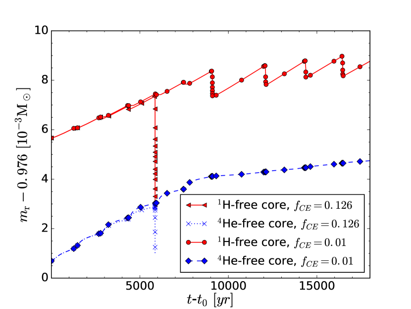
Figure 3: Evolution of H-free and He-free cores for $f_{\rm CE}=0.126$ and $f_{\rm CE}=0.01$ for $M_{\rm ZAMS}=5\,{\rm M}_{\odot}$, $Z=0.0001$ models (top). $t_{0}$ marks the beginning of the TP-AGB phase. Abundance profile and energy release due to H mixing through the bottom of the convective envelope during HDUP at $\approx(t-t_{0})=7800\mathrm{yr}$ for the case of $f_{\rm CE}=0.01$ (bottom). The vertical dashed line marks the position of the mass coordinate of the Schwarzschild boundary $m_{\mathrm{\rm SB}}$.

3 Results of stellar evolution and explosion

3.1 General properties

3.1.1 The mass and metallicity grid

The new set of models and stellar yields are all calculated with the same stellar evolution code MESA. We calculate massive star models with $M_{\rm ZAMS}=15$, $20$ and $25\,{\rm M}_{\odot}$ at $Z=0.02$ and $Z=0.01$ as an alternative to the massive star GENEC models from P16. Stellar models with $M_{\rm ZAMS}=12\,{\rm M}_{\odot}$ are added at all metallicities to cover the lower-mass end of the massive star mass range. Côté et al. (2016a) show that based on our assumption of the remnant mass distribution (cf. Sect. 2.2) adding more masses to the grid would not significantly improve galactic chemical evolution models. Côté et al. (2016a) find that the metallicity range covered is more important than the number of metallicities within that range. In addition to the $M_{\rm ZAMS}=5\,{\rm M}_{\odot}$ models in P16 we are adding intermediate and S-AGB models at all metallicities ($6$ and $7\,{\rm M}_{\odot}$). We also add a $M_{\rm ZAMS}=1\,{\rm M}_{\odot}$ models at all metallicities.

3.1.2 Stellar evolution tracks

AGB stars

The influence of metallicity on the stellar evolution is visible in the Hertzsprung-Russell diagram (HRD) with the stellar models with $M_{\rm ZAMS}=3\,{\rm M}_{\odot}$ and $M_{\rm ZAMS}=5\,{\rm M}_{\odot}$ shown in Fig. 4. The shift of the tracks of lower metallicity to higher luminosities and higher surface temperatures is the result of the larger core masses and lower opacities of the envelopes (Herwig, 2004a). The central temperature-density tracks of $M_{\rm ZAMS}=5\,{\rm M}_{\odot}$ models are separated from $M_{\rm ZAMS}=3\,{\rm M}_{\odot}$ models. The central densities $\rho_{c}$ depend on stellar mass $M$ as $\rho_{c}\propto M^{-2}$ under the assumption of constant temperature during each burning phase. Lower metallicity models behave as models with higher initial masses which is visible in the approach of the $M_{\rm ZAMS}=3\,{\rm M}_{\odot}$ tracks at low metallicities towards the $M_{\rm ZAMS}=5\,{\rm M}_{\odot}$ tracks in the central temperature-density diagram (Fig. 4).

Stellar models with $M_{\rm ZAMS}\leq 1.65\,{\rm M}_{\odot}$ for $Z=0.006$, $Z=0.001$ and $Z=0.0001$ exhibit He-core flashes. First dredge-up appears at $Z=0.006$ and $Z=0.001$ in all the AGB models but at $Z=0.0001$ only in stellar models with $M_{\rm ZAMS}\leq 2\,{\rm M}_{\odot}$. Second dredge-up occurs in models with $M_{\rm ZAMS}\geq 4\,{\rm M}_{\odot}$ and $M_{\rm ZAMS}\geq 3\,{\rm M}_{\odot}$ at $Z=0.006$ and $Z=0.001$ respectively. Core flash, first dredge-up and second dredge-up at $Z=0.006$ show the same initial-mass dependence as the AGB models at $Z=0.01$ in P16.

The average luminosity of low-mass, non-HBB stellar models follows the linear core-mass luminosity relation of Blöcker (1993) that was originally derived for $Z=0.02$ models (Fig. 5). AGB models with higher initial masses which experience HBB agree with the exponential core-mass luminosity relationship of Herwig (2004a).

AGB models with $M_{\rm ZAMS}\geq 5\,{\rm M}_{\odot}$ for $Z=0.006$, $Z=0.001$ and $Z=0.0001$ ignite C and reach the S-AGB stage. For S-AGB models with initial mass below $M_{\rm ZAMS}=7\,{\rm M}_{\odot}$ at $Z=0.006$ and below $M_{\rm ZAMS}=6\,{\rm M}_{\odot}$ at $Z=0.001$ and $Z=0.0001$ a convective C-burning flame does not appear as in stellar models of higher initial mass. In these models C burning takes place under radiative conditions. For $M_{\rm ZAMS}=4\,{\rm M}_{\odot}$ models the maximum temperatures in the C/O core do not exceed $T\approx 3\times 10^{8}\,\mathrm{K}$ which is far below the ignition temperature of $T\approx 6\times 10^{8}\,\mathrm{K}$ found by (Siess, 2007). Farmer et al. (2015) has provided a recent, detailed study of the onset of C burning, which also depends sensitively on the still very uncertain ${}^{12}\mathrm{C}$+${}^{12}\mathrm{C}$ reaction rate (see also Chen et al., 2014).

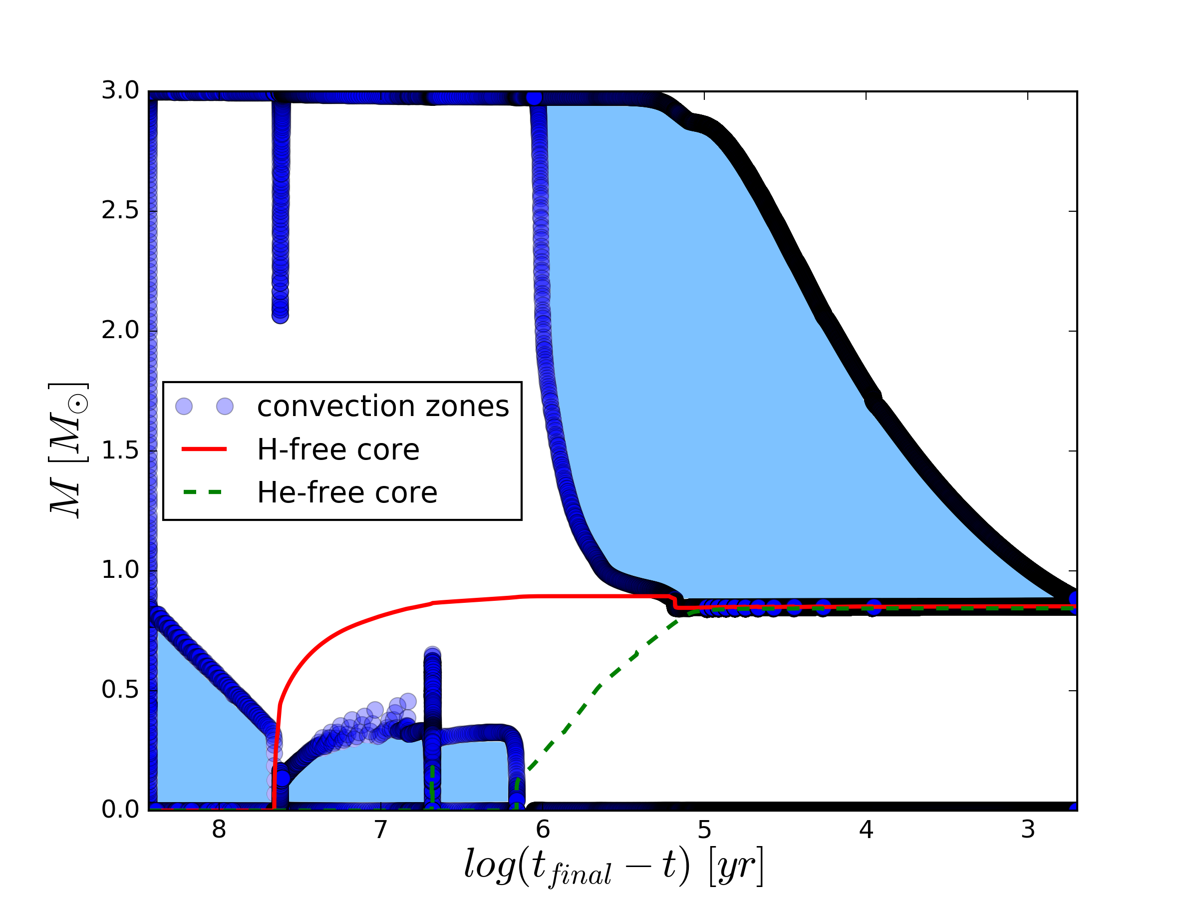
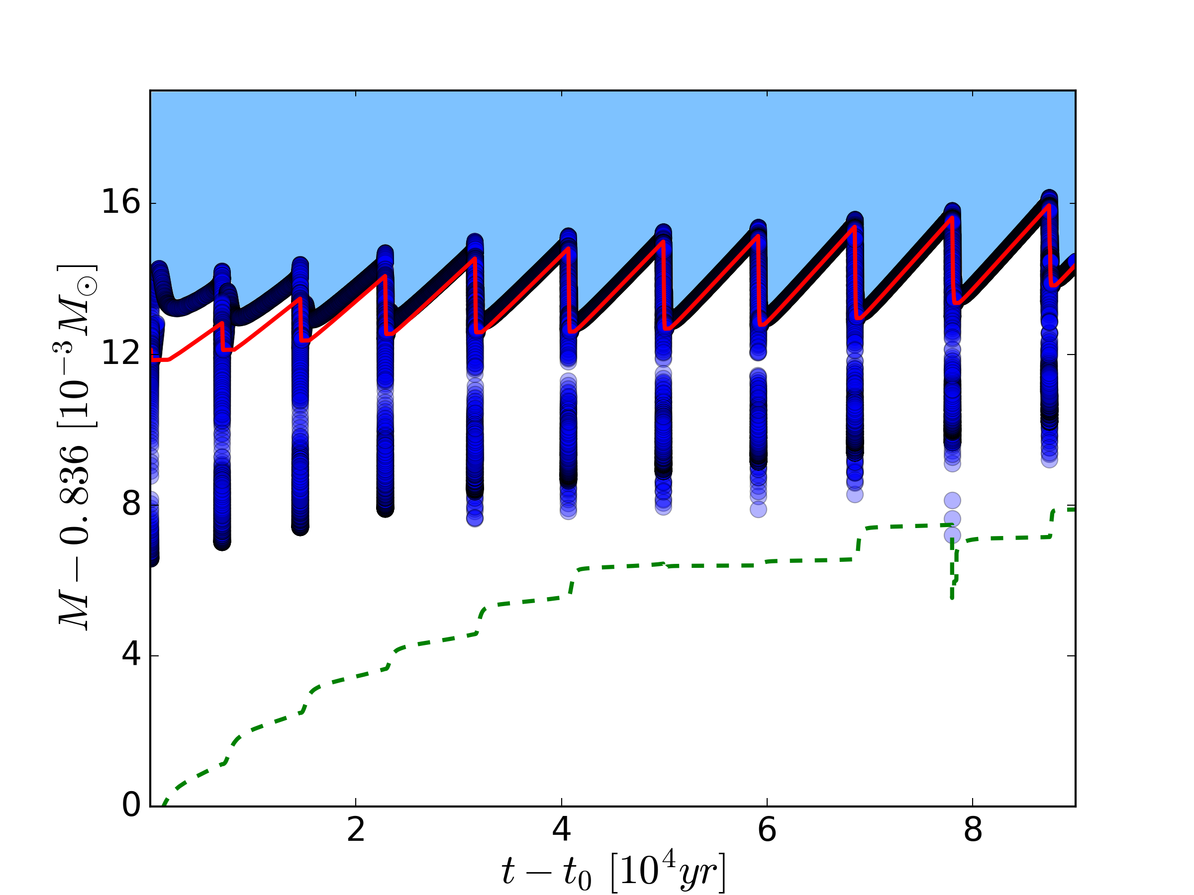
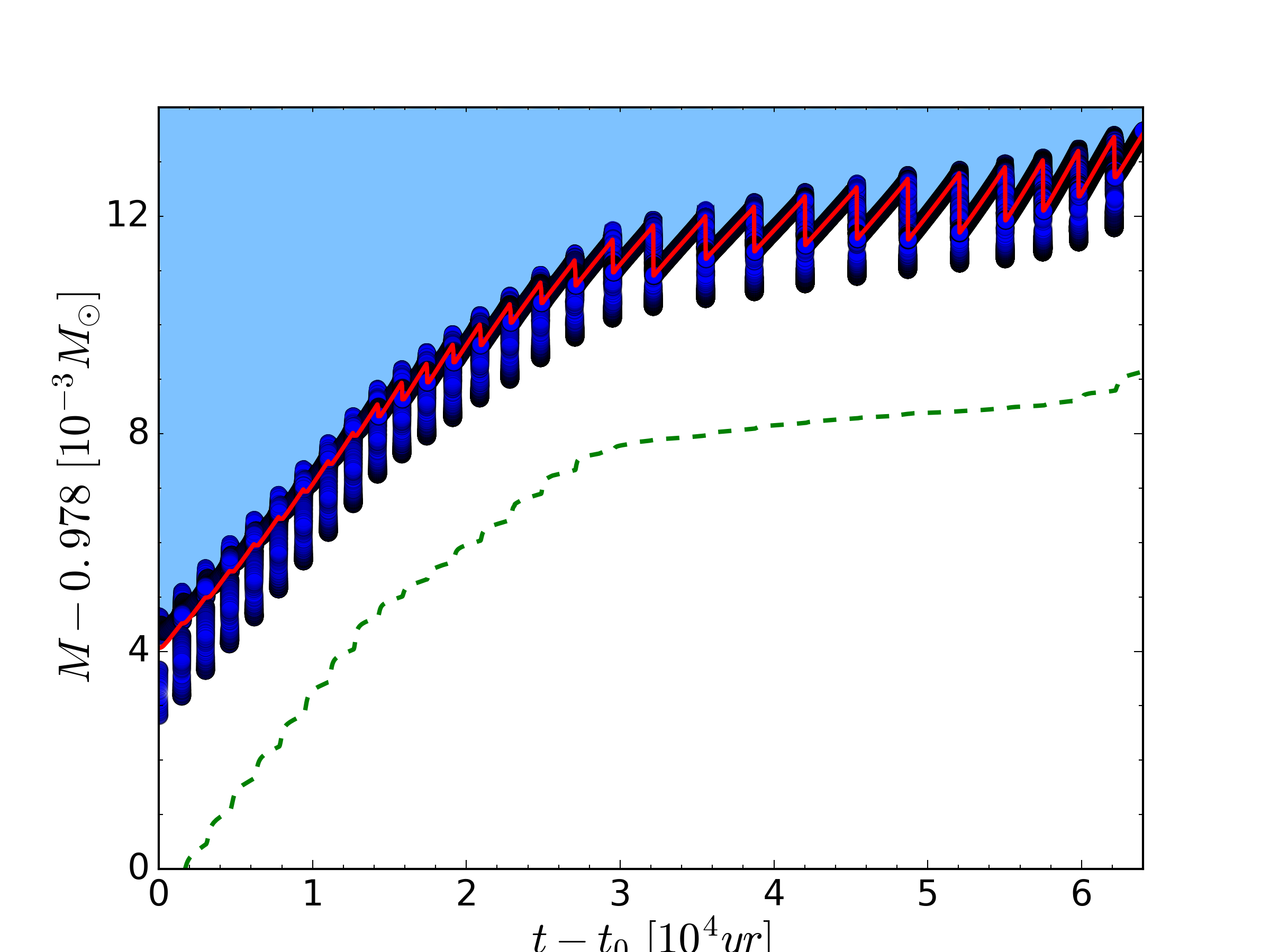
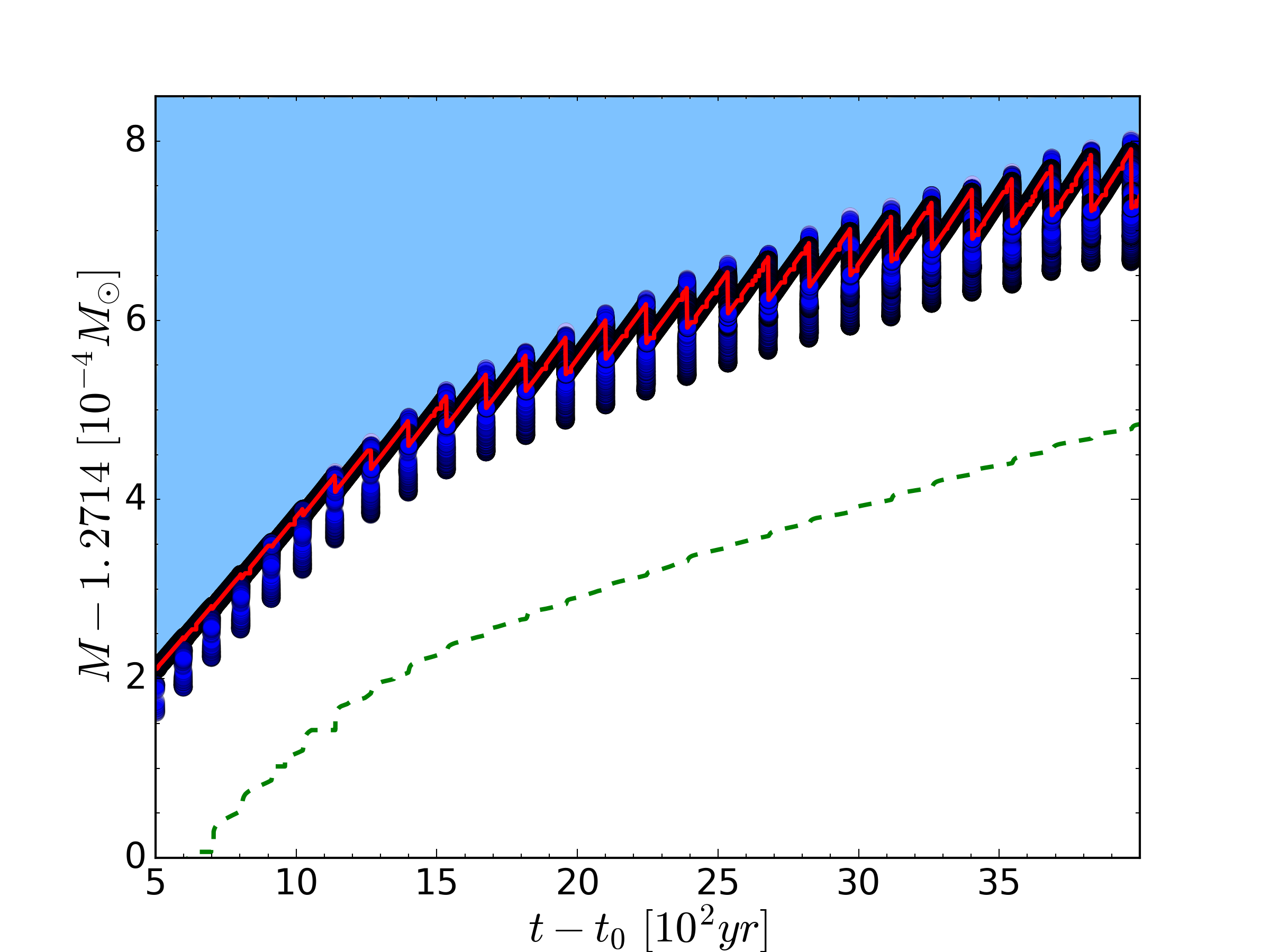
Figure 6: Kippenhahn diagrams of a $M_{\rm ZAMS}=3\,{\rm M}_{\odot}$, $Z=0.0001$ model with its pre-AGB phase (top, left) and TP-AGB phase (top, right). The H-free and He-free core boundaries are displayed by red solid and green dashed lines. The convective zones are marked in blue. $t_{0}$ and $t_{\rm final}$ are the times at the beginning and the end of the TP-AGB phase respectively. The TP-AGB phase of a massive AGB model with $M_{\rm ZAMS}=5\,{\rm M}_{\odot}$ (bottom, left) and S-AGB model with $M_{\rm ZAMS}=7\,{\rm M}_{\odot}$ (bottom, right) at $Z=0.0001$ are shown.

Model properties of the TP-AGB phase for each initial mass and metallicity are shown in Table 7. We present in Table 8 the detailed TP properties for stellar models of $Z=0.0001$. The structure evolution of models $M_{\rm ZAMS}=3\,{\rm M}_{\odot}$, $M_{\rm ZAMS}=5\,{\rm M}_{\odot}$ and $M_{\rm ZAMS}=7\,{\rm M}_{\odot}$ at $Z=0.0001$ are shown in the Kippenhahn diagrams in Fig. 6.The final core mass and lifetimes for AGB models are shown in Table 9.

We compare stellar models with $M_{\rm ZAMS}=2\,{\rm M}_{\odot}$ and $M_{\rm ZAMS}=5\,{\rm M}_{\odot}$ at $Z=0.001$ with models of Karakas (2003, K03) and Weiss & Ferguson (2009, W09) who calculated models with $M_{\rm ZAMS}=1.9\,{\rm M}_{\odot}$ and $M_{\rm ZAMS}=5\,{\rm M}_{\odot}$ based on $\alpha$-enhanced initial abundances and models of $M_{\rm ZAMS}=2\,{\rm M}_{\odot}$ and $M_{\rm ZAMS}=5\,{\rm M}_{\odot}$ of solar-scaled abundance respectively. The core mass of these two stellar models at the first TP are $0.63\,{\rm M}_{\odot}$ and $0.985\,{\rm M}_{\odot}$ while K03 obtain $0.548\,{\rm M}_{\odot}$ and $0.888\,{\rm M}_{\odot}$ and W09 get $0.494\,{\rm M}_{\odot}$ and $0.908\,{\rm M}_{\odot}$. As P16 we find larger core masses compared to K03 and W09. Our number of thermal pulses of the stellar models are 14 and 32 while K03 have 16 and 83 and W09 have 10 and 38.

The final surface C/O ratio of these stellar models is 3.243 and 3.379 compared to 8.18 and 4.48 of K03 and 3.449 and 0.772 of W09. The latter value of W09 is taken when the envelope mass is $2.642\,{\rm M}_{\odot}$ and their simulation stops. It differs from ours because in our $M_{\rm ZAMS}=5\,{\rm M}_{\odot}$ simulation the dominance of the 3DUP over weakening HBB as described in Frost et al. (1998) increases the C/O ratio from $<1$ to the large final value $>3$ over the last two thermal pulses when the stellar model loses the last $1\,{\rm M}_{\odot}$ of envelope mass. The $Z=0.006$, $M_{\rm ZAMS}=5\,{\rm M}_{\odot}$ simulation still has $0.75\,{\rm M}_{\odot}$ of envelope when it stops and the C/O ratio is $\approx 0.13$. This case does not experience the final thermal pulse where TDUP could have significantly increased the C/O ratio.

The surface C/O ratio increases due to TDUP and decreases during the interpulse HBB in massive AGB models (Lattanzio et al., 1996, 1997; Lattanzio & Boothroyd, 1997). The surface C/O ratios for stellar models of $Z=0.0001$ presented is complex (Fig. 7). While at $Z=0.02$ low mass stellar models steadily increase their surface C/O ratio (see Fig. 4 in P16), at low metallicity the first pulses can lead to a surface enhancement close to or even above the He-intershell C/O ratio as shown in Fig. 7. At low metallicity the envelope C/O ratio quickly represents that of the intershell because the total initial amount of O and C in the envelope is smaller due to the low initial metallicity. Due to a steady decrease of the C/O ratio in the He intershell over time the TDUP leads to a decline in the surface C/O ratio. Stellar models at higher metallicity such as the $M_{\rm ZAMS}=1.65\,{\rm M}_{\odot}$, $Z=0.001$ model experience only an increase of the surface C/O ratio during their evolution. For models with higher initial mass a higher C/O intershell ratio is reached which leads to a higher C/O surface enhancement in the non-HBB models.

The TDUP strength is described by the dredge-up parameter $\lambda_{\mathrm{DUP}}$ defined as $\lambda=\Delta M_{\mathrm{DUP}}/\Delta M_{\mathrm{H}}$ where $\Delta M_{\mathrm{DUP}}$ is the amount of mass dredged-up into the envelope and $\Delta M_{\rm H}$ is the increase in mass of the H-free core during the previous interpulse phase. $\lambda_{\mathrm{DUP}}$ shows a strong dependence behaviour on metallicity. In Fig. 8 we compare the stellar models with $M_{\rm ZAMS}=2\,{\rm M}_{\odot}$ and $M_{\rm ZAMS}=7\,{\rm M}_{\odot}$ at $Z=0.006$ and $Z=0.0001$. The low-mass AGB star model with lower metallicity has higher $\lambda_{\mathrm{DUP}}$ than the higher metallicity model, while the S-AGB model has higher $\lambda_{\mathrm{DUP}}$ at higher metallicity. This can be understood by considering that the dredge-up efficiency has a maximum for a core mass $\approx 0.8\,{\rm M}_{\odot}$, which at $Z=0.02$ corresponds to an initial mass of $4\,{\rm M}_{\odot}$ (P16), and in combination with the metallicity dependence of the initial to final mass relation (Fig. 9). The lower metallicity $7\,{\rm M}_{\odot}$ model has a higher core mass and therefore lower $\lambda_{\mathrm{DUP}}$. The low-mass model has also a higher core mass at lower metallicity, but here this implies larger $\lambda_{\mathrm{DUP}}$.

While the $M_{\rm ZAMS}=2\,{\rm M}_{\odot}$, $Z=0.006$ model is very similar to the $M_{\rm ZAMS}=2\,{\rm M}_{\odot}$, $Z=0.01$ model shown in Fig.  5 of P16, the $M_{\rm ZAMS}=2\,{\rm M}_{\odot}$, $Z=0.0001$ model reaches $\lambda_{\mathrm{DUP}}\approx 1$, similar to the stellar model of the same initial mass and metallicity in Herwig (2004b). The maximum of total dredged-up mass increase up to $M_{\rm ZAMS}=3\,{\rm M}_{\odot}$ for $Z=0.006$ and up to $M_{\rm ZAMS}=2\,{\rm M}_{\odot}$ for $Z=0.001$ and $Z=0.0001$. For low-mass models both quantities decline towards higher initial masses (Table 7). For comparison, Fishlock et al. (2014) found that the $M_{\rm ZAMS}=2.5\,{\rm M}_{\odot}$ and $M_{\rm ZAMS}=2.75\,{\rm M}_{\odot}$ models at $Z=0.001$ dredge-up the most material. In intermediate-mass stellar models we find lower total mass dredged up compared to Fishlock et al. (2014) who reach another maximum at $M_{\rm ZAMS}=4\,{\rm M}_{\odot}$.

The final core masses are larger at lower metallicity for most stellar models. This implies a steeper initial-final mass relation (IFMR, Fig. 9). The core masses of models from P16 are added for comparison. The IFMRs in Weiss & Ferguson (2009) which spans from $M_{\rm ZAMS}=1\,{\rm M}_{\odot}$ to $M_{\rm ZAMS}=6\,{\rm M}_{\odot}$ and covers $Z=0.02$ down to $Z=0.0005$ show in general a smaller final core mass than the present stellar models and those by P16. The spread in metallicity is more pronounced for these models. Our IFMR covers the upper part of the compiled data of observed open cluster objects shown in Fig. 10 of Weiss & Ferguson (2009). The AGB phase of the $M_{\rm ZAMS}=1\,{\rm M}_{\odot}$, $Z=0.0001$ model is terminated due to a H-ingestion event which prevents further core growth.

Massive stars

The massive star models used the same MESA code version and input parameters used by Jones et al. (2015, J15). J15 conducted a resolution study of the time steps at the end of core helium burning and we use the coarsest time step resolution that reproduced the He-free and C/O core masses. The impact of metallicity in the HRD evolution (e.g. $M_{\rm ZAMS}=15\,{\rm M}_{\odot}$ models, Fig. 4) is similar to that shown in low-mass models. There is little impact of metallicity on central temperature and density.

P16 found the final fate of massive stellar models in the mass range $M_{\rm ZAMS}=15\,{\rm M}_{\odot}$ to $M_{\rm ZAMS}=25\,{\rm M}_{\odot}$ to be the red super giant phase which is in agreement with other non-rotating models (e.g. Hirschi et al., 2004). All these massive star models experience the same phase except stellar models of $M_{\rm ZAMS}=20\,{\rm M}_{\odot}$ and $M_{\rm ZAMS}=25\,{\rm M}_{\odot}$ at $Z=0.0001$. The latter move from the blue region of the HRD into the region of yellow supergiants but not further, similar to models of Pop III stars of Heger & Woosley (2010). Due to their low metallicity these stellar models experience negligible mass loss and their intermediate convective zones are largest among all models. This leads to higher compactness which favours the blue region of the HRD (Hirschi, 2007; Peters & Hirschi, 2013).

The stellar models with $M_{\rm ZAMS}=25\,{\rm M}_{\odot}$ at all metallicities and the $M_{\rm ZAMS}=20\,{\rm M}_{\odot}$, $Z=0.01$ model burn C under radiative conditions consistent with solar-metallicity and PopIII models (Heger & Woosley, 2010, P16). The occurrence of convective core C burning in the $M_{\rm ZAMS}=20\,{\rm M}_{\odot}$, $Z=0.02$ model results from the higher luminosity of C core burning present in stellar models of higher metallicity (Hirschi, 2007; Rauscher et al., 2002; El Eid et al., 2004). Convective core C burning is present in all massive star models of lower initial mass as in P16.

The lifetimes of the core-burning stages are given in Table 10, using the definition of the lifetimes as in P16. Most burning stages are shorter for higher initial masses and lower metallicities, as expected. The final masses and the masses of the He, CO and Si cores are shown in Fig. 10, using the definitions of the core masses as in P16. The final mass increases towards lower metallicity at each initial mass. The He core masses and CO core masses show only a mild metallicity dependence compared to the clear metallicity dependence of the final mass. For some initial masses the core mass does not increase with decreasing metallicity such as the CO core masses of the stellar models with $M_{\rm ZAMS}=25\,{\rm M}_{\odot}$. The Si cores do not increase with initial mass as found for the He and CO cores. Instead, we find large variations in the metallicity of similar magnitude at different initial masses and no clear trend with metallicity (Fig. 10). This is due to the non-monotonicity for the Si core (e.g. Ugliano et al., 2012; Sukhbold & Woosley, 2014)

We compare the core masses of these stellar models with initial mass of $15\,{\rm M}_{\odot}$ and $25\,{\rm M}_{\odot}$ for $Z=0.006$ with those of Meynet & Maeder (2002, M02) at $Z=0.004$ and P16 at $Z=0.01$ in Table 11. Our He core masses are in better agreement with P16 who got larger values than M02 in spite of the metallicity difference. This is because we adopt a similar convective overshooting strength for the H-burning cores as P16 while M02 do not adopt any overshooting. More precisely, for core H and He-burning phases, in MESA models an exponentially-decaying diffusion coefficient with $f=0.022$ is used whereas in GENEC, an instantaneous penetrative overshoot with $\alpha_{\rm ov}=0.2$ H_P is used. The different treatment of convective boundary mixing explains the differences in core masses between this work and P16. The CO core masses show larger differences between this work, P16 and M02 than found for the He core masses. The mass of the Si core is in better agreement with P16 than the CO core mass (Table 11).

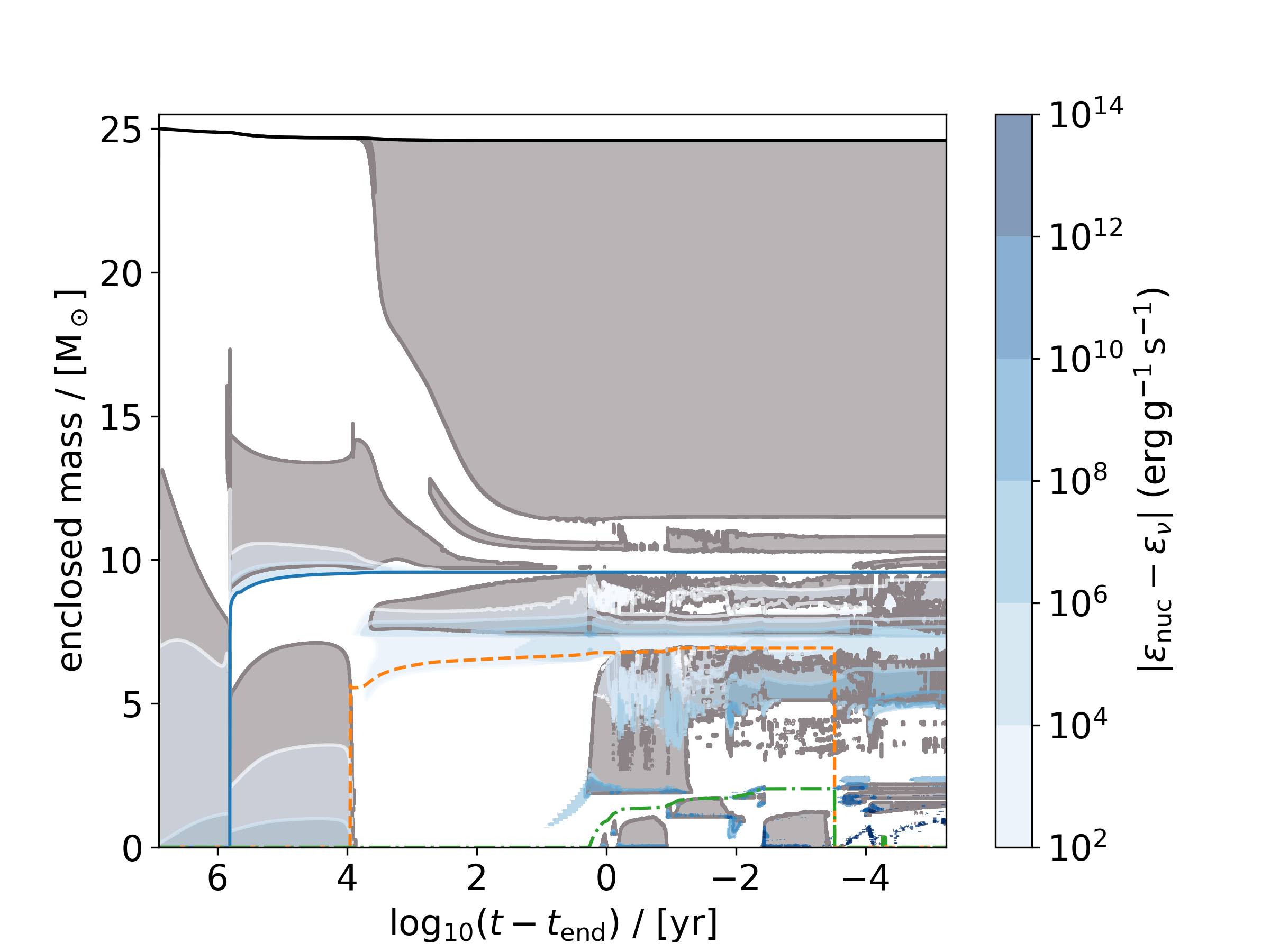
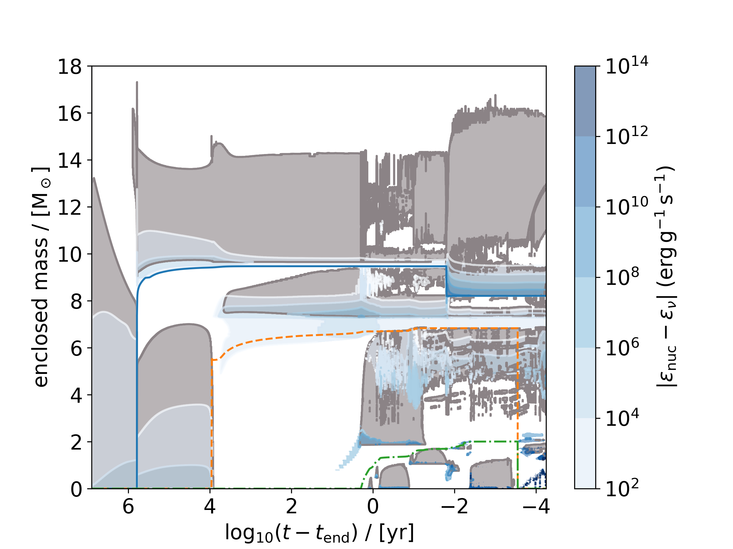
Figure 11: Kippenhahn diagrams for two stellar models with $M_{\rm ZAMS}=25\,{\rm M}_{\odot}$ at $Z=0.001$ (top) and $Z=0.0001$ (bottom). Grey areas are convective zones. The blue solid line and orange dashed line represent H-free and He-free cores respectively. The green dot-dashed line represents the C-free core. The x axis is the logarithm of the time until $t_{\mathrm{end}}$ when the infall velocity reaches $1000\,\mathrm{km/s}$. Also shown is the nuclear energy generation $\epsilon_{nuc}$ in blue shades. The specific energy loss rate due to neutrino production via nuclear reaction $\epsilon_{\nu}$ is subtracted and only positive values of $|\epsilon_{nuc}-\epsilon_{\nu}|$ are plotted.

The structural differences of stellar models with $M_{\rm ZAMS}=25\,{\rm M}_{\odot}$ at $Z=0.001$ and $Z=0.0001$ are shown in the Kippenhahn diagram in Fig. 11. Contacts between convective burning shells occur in different advanced burning stages and can have, in particular for a complete shell merger, a profound impact on stellar structure and nucleosynthesis (see Sect. 4) The contact between the convective H-burning shell and convective He-burning shell leads in the $M_{\rm ZAMS}=25\,{\rm M}_{\odot}$, $Z=0.0001$ model to a H-ingestion event. The occurrence of shell merger is affected by considerable uncertainties (Woosley et al., 2002) and requires studies with 3D hydrodynamic simulations (e.g. Meakin & Arnett, 2007; Jones et al., 2017). This point is discussed in more details below.

3.1.3 Core-collapse supernovae

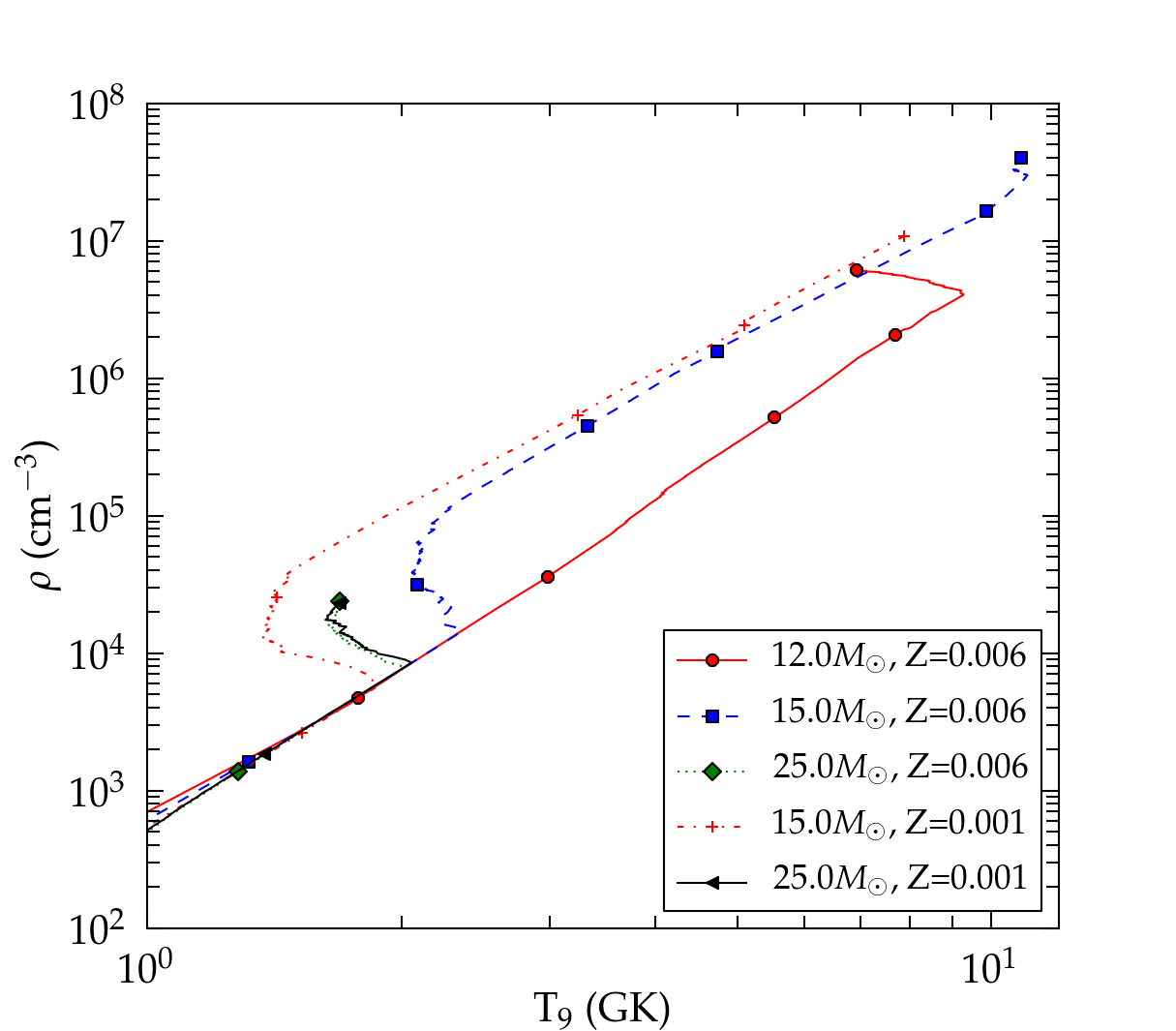
Figure 12: Maximum temperature $T_{9}$ and density $\rho$ of each zone during the CCSN explosion based on the delayed explosion prescription for massive star models of different initial masses at $Z=0.006$ and $Z=0.001$.

The explosion energy and remnant mass of a progenitor depends strongly on the pre-SN structure Fryer (1999); Müller (2016); Janka et al. (2007). The explosion properties determine the layers of the star that are ejected and the shock conditions. We compare the maximum temperatures and densities reached during the shock passage for massive star models of $Z=0.006$ and $Z=0.001$ obtained with the delayed explosion prescription (Fig. 12). The shock temperature for stellar models with $M_{\rm ZAMS}=12\,{\rm M}_{\odot}$ and $M_{\rm ZAMS}=15\,{\rm M}_{\odot}$ at $Z=0.006$ are the largest of all metallicities. Up to $Z=0.006$ stellar models with $M_{\rm ZAMS}=15\,{\rm M}_{\odot}$ reach the highest shock temperatures and densities followed by the $M_{\rm ZAMS}=12\,{\rm M}_{\odot}$ models but at higher metallicity the trend is reversed.

The pre-SN structure of these stellar models do not always show trends with metallicity (Fig. 13) and the same counts for the shock temperatures. There is no trend in the Fe-core mass with mass and metallicity and instead the stellar models with $M_{\rm ZAMS}=20\,{\rm M}_{\odot}$ show the largest Fe core masses (Fig. 13). Recent studies show that there is no monotonous compactness trend with initial mass and metallicity (Ugliano et al., 2012; Sukhbold & Woosley, 2014; Sukhbold et al., 2016).

Under the convective engine paradigm (Herant et al., 1994), whether or not the model explodes depends sensitively on the ram pressure of the stellar material falling onto the outer edge of the convective region (Fryer, 1999). To drive an explosion, the energy in the convective region must overcome this ram pressure and the energy in the convective region when this occurs determines the explosion energy of the supernova. Typically, the energy in the convective region required to overcome an accretion rate of $0.5\mathrm{\,{\rm M}_{\odot}\mathrm{s^{-1}}}$ is $1-3\times 10^{51}\,{\rm erg}$. The Fryer et al. (2012) formalism assumes that the energy in the convective region increases over time (either on rapid or delayed timescales) and assumed that, when the pressure in the convective region exceeded the ram pressure, an explosion was launched.

To determine this pressure and, hence, the likelihood of the star exploding, we calculate the accretion rate as a function of time (Fig. 14). Just based on these accretion rates, we see that the convective engine is likely to explode both the $M_{\rm ZAMS}=12$ and $M_{\rm ZAMS}=15\,{\rm M}_{\odot}$ progenitors at z=0.02 and z=0.01. Although the $M_{\rm ZAMS}=12\,{\rm M}_{\odot}$ will explode at all metallicities, it becomes increasingly difficult to drive explosions in the $M_{\rm ZAMS}=15\,{\rm M}_{\odot}$ at lower metallicities. Typically, the high accretion rates for the $M_{\rm ZAMS}=20$ and $M_{\rm ZAMS}=25\,{\rm M}_{\odot}$ models make them difficult to explode and we expect no or weak explosions from these models. The exception is the z=0.01 metallicity $M_{\rm ZAMS}=20\,{\rm M}_{\odot}$ star where a shell merger occurred. This altered the density profile at collapse sufficiently to make this star more-likely to explode, but the high accretion rates at late times is indicative of a large density that may lead to considerable fallback.

The mass at the launch of the explosion can be estimated by looking at the accretion rate as a function of accreted mass. The unique feature of our $M_{\rm ZAMS}=12\,{\rm M}_{\odot}$ MESA progenitor is evident here. Its core is larger than other progenitors in the literature and it is more likely to make more massive neutron stars. When the accretion rate falls below $0.5\,{\rm M}_{\odot}\mathrm{s^{-1}}$, the accreted baryonic mass is $\approx 1.7$ to $1.9\,{\rm M}_{\odot}$, corresponding to a gravitational mass of $\approx 1.5$ to $1.7\,{\rm M}_{\odot}$. In the $Z=0.01$ sequence the $M_{\rm ZAMS}=12$, $15\,{\rm M}_{\odot}$ and $20\,{\rm M}_{\odot}$ models experience O-C shell mergers (Sect. 4.4). The consequence is a rapid decline of the mass accretion rate at the location of the bottom of the merged shell. At least at the launch of the explosion, the $M_{\rm ZAMS}=20\,{\rm M}_{\odot}$ stellar model can produce a smaller remnant than our $M_{\rm ZAMS}=12\,{\rm M}_{\odot}$ and $M_{\rm ZAMS}=15\,{\rm M}_{\odot}$ models.

The maximum temperatures and densities of these delayed explosions at $Z=0.02$ are similar to those shown in Fig. 31 of P16 for stellar models with $M_{\rm ZAMS}/\,{\rm M}_{\odot}$ = 15, 20, 25. We find qualitatively the same increase with initial mass but lower explosion temperatures except for the model with $M_{\rm ZAMS}=25\,{\rm M}_{\odot}$. We attribute the different explosion conditions to the different pre-SN structures which were calculated with different stellar evolution codes. The density in Fe core layers at collapse of our $M_{\rm ZAMS}=25\,{\rm M}_{\odot}$, $Z=0.02$ model is more than $1\,\mathrm{dex}$ larger than in the model of P16 that were calculated with the GENEC code and for which the pre-collapse phase was not modeled (Fig. 13). The densities of the O shell layers are in better agreement.

3.2 Features at low metallicity

3.2.1 H ingestion

H-ingestion episodes are found in many phases of stellar evolution particularly in low and zero-metallicity AGB and He-core flash models (e.g. Fujimoto et al., 2000; Cristallo et al., 2009; Campbell et al., 2010), in very late thermal pulses in models of post-AGB stars (Herwig et al., 1999), in S-AGB stars (cf. Sect. 3.2.3, Jones et al., 2016). The mixing between the H-burning shell and He-burning shell in massive stars have been reported for models at low metallicity in Woosley & Weaver (1995); Hirschi (2007) and for Pop III models in Heger & Woosley (2010).

At the first TP of the $M_{\rm ZAMS}=1\,{\rm M}_{\odot}$, $Z=0.0001$ model the PDCZ penetrates slightly into the H-rich envelope. The protons from the envelope are mixed into the PDCZ and react with ${}^{\makebox[7.0pt][r]{$\scriptstyle 12$}}_{\makebox[7.0pt][r]{$\scriptstyle$}}\mathrm{C}$ and form ${}^{\makebox[7.0pt][r]{$\scriptstyle 13$}}_{\makebox[7.0pt][r]{$\scriptstyle$}}\mathrm{N}$. The latter decays to ${}^{\makebox[7.0pt][r]{$\scriptstyle 13$}}_{\makebox[7.0pt][r]{$\scriptstyle$}}\mathrm{C}$ which activates the ${}^{\makebox[7.0pt][r]{$\scriptstyle 13$}}_{\makebox[7.0pt][r]{$\scriptstyle$}}\mathrm{C}$($\alpha$,n) neutron source. This leads to the production of heavy elements. In the following TP the convective He-burning zone penetrates again into the envelope which leads to the ingestion of much larger amounts of H than previously and stronger surface enrichment of He intershell material. A H-ingestion flash (HIF) with a peak luminosity of $L_{\mathrm{H}}\approx 10^{10}\,\,{\rm L}_{\odot}$ occurs. This HIF terminates the AGB phase and is shown in the Kippenhahn diagram in Fig. 15. The conditions are similar to those found in Iwamoto et al. (2004).

The $M_{\rm ZAMS}=1\,{\rm M}_{\odot}$, $Z=0.006$ model experiences a He-shell flash when it leaves its horizontal post-AGB evolution towards the white dwarf (WD) cooling track (Iben et al., 1983; Iben & MacDonald, 1995). This Very-late Thermal Pulse (VLTP, Herwig, 2001a) causes the PDCZ to reach into the H-rich envelope, leading to H ingestion, and a born-again phase (Herwig et al., 1999, 2011). The calculation is terminated six years after the H ingestion due to convergence problems. The H ingestion leads to the production of heavy elements up to the first s-process peak in the He intershell which are mixed to the surface. Due to the energy release of H burning a connected stable layer forms within the PDCZ and the convective zone splits into two. VLTP events like this are not expected to influence significantly the composition of the stellar ejecta and the total yields, because the remaining envelope is small and the cool born-again evolution phase is short. VLTP events have been shown to posses significant non-radial, global oscillations (Herwig et al., 2014) which make their one-dimensional stellar evolution modelling unreliable. This applies equally to H-ingestion flashes in low-metallicity AGB stars (Woodward et al.  in prep.).

In the S-AGB models the time between TP and TDUP becomes shorter for lower metallicity, and this may lead to H-ingestion events (Jones et al., 2016). Due to the choice of convective boundary mixing parameters this happens only occasionally in these models, below $Z=0.01$. For example, H ingestion happens during the 29th TP of the $M_{\rm ZAMS}=7\,{\rm M}_{\odot}$, $Z=0.001$ model. For this thermal pulse we obtain neutron densities of up to $N_{n}=10^{12}\,\mathrm{cm}^{-3}$ in the deepest layers of the PDCZ, for about five days. The splitting of the PDCZ due to H burning prevents the transport of material from the deep layers to the surface. Since these events are not frequent in these $7\,{\rm M}_{\odot}$ models, the nucleosynthesis of HIFs does not contribute significantly to the stellar yields presented here.

Stellar models of $M_{\rm ZAMS}=20\,{\rm M}_{\odot}$ and $M_{\rm ZAMS}=25\,{\rm M}_{\odot}$ of $Z=0.0001$ experience H ingestion at the beginning of convective C shell burning and during O shell burning respectively. At higher metallicity we find H ingestion in the $M_{\rm ZAMS}=20\,{\rm M}_{\odot}$, $Z=0.001$ model and in the $M_{\rm ZAMS}=12\,{\rm M}_{\odot}$, $Z=0.006$ model. In both models H ingestion events occur during Si shell burning. These H-ingestion, or sometimes H/He-shell mixing events happen without the application of CBM at the boundaries of the convective He shell (as all other convective boundaries post-He core burning). The penetration into the convective He-burning layer is visible for the $M_{\rm ZAMS}=25\,{\rm M}_{\odot}$, $Z=0.0001$ model in Fig. 11. The resulting energy release leads to the formation of two extended convective regions which persist until collapse. We find at the bottom of the He-shell convective zone neutron densities close to $N_{n}=10^{11}\,\mathrm{cm}^{-3}$ which remain for days until core collapse. There is only a minor production of heavy elements but lighter elements such as F are effectively produced and contribute a relevant fraction of the total stellar yields of this stellar model.

Detailed investigations of the nucleosynthesis and 3D stellar hydrodynamics of the H-ingestion event in the post-AGB star Sakurai’s object (Herwig et al., 2011; Herwig et al., 2014) have shown that the assumption of spherical symmetry and the approximation of mixing via mixing length theory of convection are not appropriate. This is consistent with the failure of such 1D models to reproduce several key observables, such as light-curve and heavy-element abundance patterns of Sakurai’s object. This suggests that the properties of H-ingestion events in this stellar yield grid are indicative at best, and need to be investigated further through 3D hydrodynamics simulations.

3.2.2 Hot bottom burning

The temperature at the bottom of the convective envelope $T_{\mathrm{CEB}}$ increases with increasing initial mass and decreasing metallicity as shown in Fig. 5 and reaches up to $T_{\mathrm{CEB}}=2.3\times 10^{8}\,\mathrm{K}$. In S-AGB models with $M_{\rm ZAMS}=7\,{\rm M}_{\odot}$ at $Z=0.0001$ and $Z=0.006$ temperatures reach more than $T_{\mathrm{CEB}}=1.5\times 10^{8}\,\mathrm{K}$ which allows the activation of the NeNa and MgAl cycles. The $M_{\rm ZAMS}=3\,{\rm M}_{\odot}$, $Z=0.0001$ model reaches $T_{\mathrm{CEB}}=4\times 10^{7}\,\mathrm{K}$ which leads to HBB. Models of the same mass but of higher metallicity do not experience HBB (Table 7). The threshold initial mass for HBB in Ventura et al. (2013) was found to be $M_{\rm ZAMS}=3\,{\rm M}_{\odot}$ at $Z=0.0003$ and $M_{\rm ZAMS}=3.5\,{\rm M}_{\odot}$ at $Z=0.008$ which is similar to our findings. HBB is active in stellar models of masses as low as $M_{\rm ZAMS}=3\,{\rm M}_{\odot}$ in agreement with models at $Z=0.001$ of Fishlock et al. (2014).

3.2.3 Effects of hot dredge-up and dredge-out

Herwig (2004b) find that hot dredge-up is characterized by extreme H-burning luminosities of $L_{\mathrm{H}}=2\times 10^{6}\,\,{\rm L}_{\odot}$ for their $M_{\rm ZAMS}=5\,{\rm M}_{\odot}$, $Z=0.0001$ model. For stellar models with $M_{\rm ZAMS}\leq 4\,{\rm M}_{\odot}$ and $Z=0.0001$ $L_{\mathrm{H}}$ often exceeds the peak He-burning luminosities of the TP. Under the most extreme conditions in models with $M_{\rm ZAMS}=6\,{\rm M}_{\odot}$ and $M_{\rm ZAMS}=7\,{\rm M}_{\odot}$ we find $L_{\mathrm{H}}>10^{9}\,\,{\rm L}_{\odot}$. At higher metallicities $L_{\mathrm{H}}$ is lower. Because of the reduced CBM efficiency $f_{\mathrm{CE}}$ in massive AGB and S-AGB models (see Sect. 2.1.4) the size of ${}^{13}\mathrm{C}$ pocket decreases substantially with increasing initial mass. Additionally, the pressure scale height at the core-envelope interface decreases with increasing initial mass which leads to a further decrease of the CBM in the parametrized model. This leads to ${}^{13}\mathrm{C}$ pockets in S-AGB models below $10^{-7}\,\,{\rm M}_{\odot}$ at $Z=0.0001$.

Dredge-out is found in the most massive AGB models during second DUP when the convective He-burning shell grows in mass and merges with the convective envelope. This leads to the enrichment of the surface with products of He-shell burning (Ritossa et al., 1999). H can be entrained into the He-burning convection zone and ignite as a flash. This is another H-ingestion event (Gil-Pons & Doherty, 2010; Jones et al., 2016). We find dredge-out in S-AGB models with $M_{\rm ZAMS}=7\,{\rm M}_{\odot}$ at $Z=0.001$ and $Z=0.0001$. The flash at $Z=0.0001$ produces a peak in luminosity of up to $L_{\mathrm{H}}\approx 10^{8}\,\,{\rm L}_{\odot}$. The maximum H-burning luminosities agree well with Jones et al. (2016). The initial masses of our stellar models with dredge-out are below the lower initial mass limit of dredge-out of $M_{\rm ZAMS}\gtrapprox 9\,{\rm M}_{\odot}$ as reported by Gil-Pons & Doherty (2010), presumably due to difference in the core overshooting prescription.

3.2.4 Carbon flame quenching in S-AGB stars

In the $M_{\rm ZAMS}=7\,{\rm M}_{\odot}$, $Z=0.006$ S-AGB model the propagation of the C flame toward the center is quenched (Denissenkov et al., 2013). The C-flame quenching depends sensitively on the assumption of CBM, which is essentially unconstrained. If CBM at the bottom of the C-burning shell is efficient enough to quench the flame, then the result is a hybrid core. It consists of a inner C-O core of $\approx 0.145\,{\rm M}_{\odot}$ surrounded by thicker layers of O, Ne and Mg. For stellar models with $M_{\rm ZAMS}=7\,{\rm M}_{\odot}$ the first C-burning flash occurs at $Z=0.0001$ closer to the center than at higher metallicity. The C burning moves outward in mass through a series of convective C-shell burning episodes. The location of the first C ignition is further outwards for models of higher metallicity due to the higher degeneracy of the lower core masses (García-Berro et al., 1997; Siess, 2007). The onset of C burning coincides with the beginning of the second DUP for the $M_{\rm ZAMS}=7\,{\rm M}_{\odot}$, $Z=0.006$ model. At higher metallicity the C burning starts earlier than at lower metallicity. The difference in metallicity has a qualitatively similar effect on convective C burning as the difference in initial mass between $M_{\rm ZAMS}=7.6\,{\rm M}_{\odot}$ and $M_{\rm ZAMS}=9\,{\rm M}_{\odot}$ shown in Fig. 3 in Farmer et al. (2015). Possible implications of hybrid WDs are discussed in Denissenkov et al. (2017).

$M_{\rm ZAMS}$	$m_{c}$	$\log L_{\ast}$	$R_{\ast}$	$N_{\rm TP}$	$N_{\rm TDUP}$	$t_{\rm TPI}$	$\Delta M_{\rm Dmax}$	$M_{D}$	$t_{ip}$	$M_{\rm lost}$	$\log T_{\rm CEB,max}$	$\log T_{\rm PDCZ,max}$	$M_{\rm PDCZ}$	$\log L_{\rm He,max}$	$\log L_{\rm max}$
[$M_{\odot}$]	[$M_{\odot}$]	[$L_{\odot}$]	[$R_{\odot}$]			[$10^{6}\,{\rm yr}$]	[$10^{-2}\,\,{\rm M}_{\odot}$]	[$10^{-2}\,\,{\rm M}_{\odot}$]	[${\rm yr}$]	[$M_{\odot}$]	[${\rm K}$]	[${\rm K}$]	[$10^{-2}\,\,{\rm M}_{\odot}$]	[$L_{\odot}$]	[$L_{\odot}$]
Z=0.0001
1.00	0.532	3.19	75	2	1	5.726E+03	2.485	2.485	274820	0.33	6.266	8.312	3.986	6.72	3.63
1.65	0.589	3.77	161	12	11	1.231E+03	0.702	5.482	91155	0.99	6.870	8.461	2.956	7.53	4.05
2.00	0.655	3.97	205	11	10	7.494E+02	0.895	6.242	56131	1.31	7.114	8.490	1.906	7.89	4.14
3.00	0.848	4.29	295	11	10	2.722E+02	0.242	1.897	8765	2.01	7.715	8.514	0.569	7.63	4.48
4.00	0.899	4.43	345	19	18	1.414E+02	0.246	2.506	5253	3.01	7.979	8.541	0.376	8.00	4.55
5.00	0.982	4.59	413	29	20	8.805E+01	0.111	1.331	2228	3.93	8.057	8.553	0.165	7.82	4.76
6.00	1.124	4.83	572	19	16	6.115E+01	0.038	0.428	824	4.52	8.141	8.561	0.049	7.07	4.96
7.00	1.272	5.05	743	27	21	4.557E+01	0.007	0.091	134	4.70	8.369	8.597	0.009	6.72	5.10
$M_{ini}$: Initial stellar mass.
$m_{c}$: H-free core mass at the first TP.
$L_{\ast}$: Approximated mean stellar luminosity.
$R_{\ast}$ : Approximated mean stellar radius.
$N_{\rm TP}$: Number of TPs.
$N_{\rm TDUP}$ : Number of TPs with TDUP.
$t_{\rm TPI}$: Time at first TP.
$\Delta M_{\rm Dmax}$: Maximum dredged-up mass after a single TP.
$M_{D}$: Total dredged-up mass of all TPs.
$t_{ip}$ : Average interpulse duration of TPs.
$M_{\rm lost}$: Total mass lost during the TP-AGB phase.
$T_{\rm PDCZ,max}$: Maximum temperature during the TP-AGB phase.
$M_{\rm PDCZ}$: Maximum size of PDCZ.
$\log L_{\rm He,max}$: Maximum He luminosity during TP-AGB phase.
$\log L_{max}$: Maximum total luminosity during TP-AGB phase.

Table 7: TP-AGB properties for models at $Z=0.0001$. Properties for $Z=0.006$, $0.001$ are available with the online version of the paper (Appendix A).

TP	$t_{\rm TP}$	$\log T_{\rm FBOT}$	$\log T_{\rm HES}$	$\log T_{\rm HS}$	$\log T_{\rm CEB}$	$m_{\rm FBOT}$	$m_{\rm HTP}$	$m_{\rm D,max}$	$M_{\ast}$
	[${\rm yr}$]	[${\rm K}$]	[${\rm K}$]	[${\rm K}$]	[${\rm K}$]	[$M_{\odot}$]	[$M_{\odot}$]	[$M_{\odot}$]	[$M_{\odot}$]
$M=1.0M_{\odot}$
1	0.00E+00	8.31	8.16	7.75	5.98	0.4926	0.5324	0.5358	0.867
2	2.75E+05	8.09	8.05	8.05	5.99	0.5218	0.5374	0.0000	0.867
TP: TP number.
$t_{\rm TP}$: Time since the first TP.
$T_{\rm FBOT}$: Largest temperature at the bottom of the PDCZ.
$T_{\rm HES}$: Temperature in the He-burning shell during deepest extend of TDUP.
$T_{\rm CEB}$: Temperature at the bottom of the convective envelope during deepest extend of TDUP.
$m_{\rm FBOT}$: Minimum mass coordinate of the bottom of the He-flash convective zone.
$m_{\rm D,max}$: Mass coordinate of the H-free core at the time of the TP.
$M_{\ast}$: Stellar mass at the TP.

Table 8: Model properties of the TP-AGB phase for $Z=0.0001$. Properties for $Z=0.006$, $0.001$ are available with the online version of the paper (Appendix A).

$M_{\rm ZAMS}$	$M_{\mathrm{final}}$	$\tau_{\mathrm{total}}$
[$\,{\rm M}_{\odot}$]	[$\,{\rm M}_{\odot}$]	[${\rm yr}$]
1.0	0.592	5.670E+09
1.65	0.637	1.211E+09
2.0	0.665	6.972E+08
3.0	0.852	2.471E+08
4.0	0.905	1.347E+08
5.0	0.992	8.123E+07
6.0	1.125	5.642E+07
7.0	1.272	4.217E+07

Table 9: Final core masses $M_{\mathrm{final}}$ and total lifetime $\tau_{\mathrm{total}}$ for $Z=0.0001$. We provide tables for other metallicities online (Appendix A).

$M_{\rm ZAMS}$	$\tau_{\mathrm{H}}$	$\tau_{\mathrm{He}}$	$\tau_{\mathrm{C}}$	$\tau_{\mathrm{Ne}}$	$\tau_{\mathrm{O}}$	$\tau_{\mathrm{Si}}$	$\tau_{\mathrm{total}}$
Z = 0.02
12	1.742E+07	1.669E+06	1.046E+04	1.046E+01	2.973E+00	1.895E-01	1.935E+07
15	1.243E+07	1.250E+06	1.835E+03	2.829E+00	1.361E+00	8.840E-02	1.386E+07
20	8.687E+06	8.209E+05	1.270E+02	1.811E+00	7.086E-01	5.071E-02	9.596E+06
25	6.873E+06	6.426E+05	2.525E+02	5.303E-01	1.390E-01	1.385E-02	7.585E+06

Table 10: Lifetimes of major central burning stages of massive star models. Shown are lifetimes for H burning, $\tau_{\mathrm{H}}$, He burning, $\tau_{\mathrm{He}}$, C burning, $\tau_{\mathrm{C}}$, Ne burning $\tau_{\mathrm{Ne}}$, O burning, $\tau_{\mathrm{O}}$, Si burning, $\tau_{\mathrm{Si}}$, and the total lifetime of the stellar models, $\tau_{\mathrm{total}}$. Times in $\mathrm{yr}$. The complete table is available with the online version of the paper.

$M_{\rm ZAMS}$	$15\,{\rm M}_{\odot}$			$25\,{\rm M}_{\odot}$
	this work	M02	P16	this work	M02	P16
$M_{\mathrm{\alpha}}$	5.09	4.45	4.81	9.66	8.44	9.39
$M_{\mathrm{CO}}$	3.27	2.27	2.84	7.26	5.35	6.45
$M_{\mathrm{Si}}$	2.02		1.7	1.99		1.85

Table 11: Comparison of the He core mass ($M_{\mathrm{\alpha}}$), CO core mass ($M_{\mathrm{CO}}$) and Si core mass $M_{\mathrm{Si}}$ of massive star models at $Z=0.006$ of this work with models at $Z=0.004$ of M02 and models at $Z=0.01$ of P16. Core masses are in $\,{\rm M}_{\odot}$.

Figure 4: Comparison of HRD’s for AGB models with $M_{\rm ZAMS}=3\,{\rm M}_{\odot}$ and $M_{\rm ZAMS}=5\,{\rm M}_{\odot}$ (top) and massive star models with $M_{\rm ZAMS}=15\,{\rm M}_{\odot}$ (middle) for $Z=0.006$, $Z=0.001$ and $Z=0.0001$. Central temperatures $T_{c}$ and densities $\rho_{c}$ for those AGB models (bottom).

Figure 5: Average luminosity versus average core mass of the TP-AGB stage for stellar models at $Z=0.006,0.001$ and $0.0001$ in comparison with the linear and exponential core-mass luminosity relations of Blöcker (1993, CMLR B93) and Herwig (2004a, CMLR H04) respectively (top). The luminosities of low-mass models are higher than the the classical CMLR because of third dredge-up (Herwig et al., 1998). Maximum temperature at the bottom of the convective envelope $T_{\rm CEB}$ versus final core mass during the AGB evolution (bottom).

Figure 7: Surface C/O ratio versus total stellar mass for $Z=0.0001$ (top). The He intershell and surface C/O ratio for each TP of two stellar models with $M_{\rm ZAMS}=1.65\,{\rm M}_{\odot}$ and $M_{\rm ZAMS}=2\,{\rm M}_{\odot}$ (bottom).

Figure 8: Metallicity dependence of the DUP parameter $\lambda$ shown at the example of low-mass AGB models and a S-AGB models with $M_{\rm ZAMS}=2\,{\rm M}_{\odot}$ and $M_{\rm ZAMS}=7\,{\rm M}_{\odot}$ for $Z=0.0001$ and $Z=0.006$.

Figure 9: Initial-final mass relation for AGB models of this work with AGB models between $M_{\rm ZAMS}=1.65\,{\rm M}_{\odot}$ and $M_{\rm ZAMS}=5\,{\rm M}_{\odot}$ at $Z=0.02$ and $Z=0.01$ from P16.

Figure 10: Core masses versus initial mass at the time of core collapse for massive star models. For each model the final mass ($M_{\mathrm{final}}$), He core mass ($M_{\mathrm{\alpha}}$), CO core mass ($M_{\mathrm{CO}}$) and Si core mass ($M_{\mathrm{Si}}$) are shown.

Figure 13: Density profiles at core collapse when the infall velocity reaches $1000\,\mathrm{km/s}$ for massive star models at $Z$=0.02, 0.01, 0.001, 0.0001. The 1 to 8 Mo range is shown. This includes, from left to right, from the outer part of the Fe core to at least the end of the O shell. Comparison of the density profiles at the end of Si core burning of our stellar model with $M_{\rm ZAMS}=25\,{\rm M}_{\odot}$ at $Z=0.02$ computed with the MESA code (MES, this work) and the model provided by P16 and calculated with the GENEC code (GNV).

Figure 14: Free-fall mass accretion rates for all massive star models for four metallicities at the time of collapse. The time offset for the $12\,{\rm M}_{\odot}$ models is due to the larger core mass and associated choice of the mass cut (Sect. 2.2).

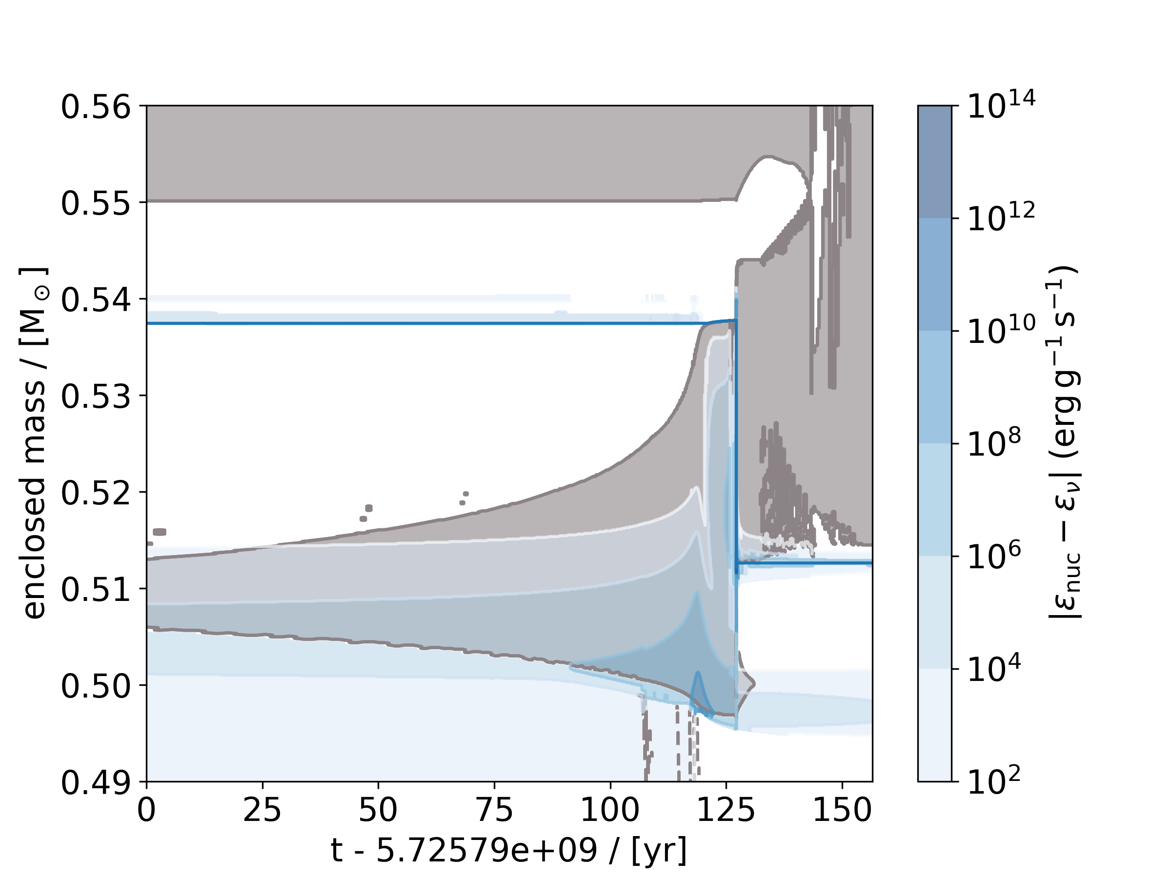
Figure 15: H-ingestion in the $M_{\rm ZAMS}=1\,{\rm M}_{\odot}$, $Z=0.0001$ model. The blue solid line represents the H-free core. The H ingestion during the second thermal pulse terminates the TP-AGB phase.

4 Post-processing nucleosynthesis results

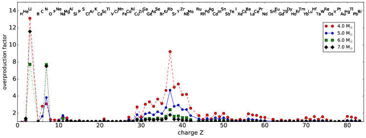
Figure 16: Overproduction factors versus charge number of final yields of AGB models at $Z=0.02$ with models of $M_{\rm ZAMS}/\,{\rm M}_{\odot}$ = 1.65, 2, 3, 4, 5 of P16.

This section is complementary to the discussion in P16 ($Z\geq 0.01$) and the main focus are results obtained for $Z\leq 0.006$. Processes covered include, among others, the weak and main s process (Käppeler et al., 1989; Straniero et al., 1995; Gallino et al., 1998; Käppeler et al., 2011), the $\alpha$-process (Woosley & Hoffman, 1992; Magkotsios et al., 2010) and $\gamma$ process (Rayet et al., 1995; Arnould & Goriely, 2003). Overproduction factors ${\rm OP}_{\rm im}$ (Sect. 2.3) provide an overview of which stellar models at which metallicity contribute to which elements/isotopes (Figs. 16 through 23).

Final yields with their wind contribution, pre-SN and SN contribution (Sect. 2.3) are shown for $Z=0.0001$ in Table 12, and all others are available online (Appendix A). In this section we briefly discuss the results from our post-process calculations.

4.1 First dredge-up, second dredge-up and dredge-out

In the AGB models with $M_{\rm ZAMS}=1.65\,{\rm M}_{\odot}$, He originates mostly from the first dredge-up. For higher initial masses the contribution of the second dredge-up increases while the contribution of the first dredge-up decreases. Stellar models of the same initial mass experience deeper first dredge-up at higher metallicity. The initial mass above which the second dredge-up is responsible for most He production is $M_{\rm ZAMS}=2\,{\rm M}_{\odot}$ at $Z=0.0001$ and $M_{\rm ZAMS}=3\,{\rm M}_{\odot}$ at $Z=0.006$. The largest overproduction of He in AGB models occurs at the highest initial masses.

The C overproduction factors of AGB models peak at $M_{\rm ZAMS}=2\,{\rm M}_{\odot}$ for $Z=0.006$ and $Z=0.001$ and at $M_{\rm ZAMS}=1.65\,{\rm M}_{\odot}$ for $Z=0.0001$ (Fig. 24). The total amount of dredged-up material reaches a maximum in these three initial stellar models (Table 7). The largest overproduction factors of AGB models are slightly larger than those found in massive star models. We find dredge-out (Ritossa et al., 1999; Jones et al., 2016) in stellar models with initial mass of $7\,{\rm M}_{\odot}$ at $Z=0.001$ and $Z=0.0001$ where it is the main source of surface enrichment of C.

In the lowest-metallicity cases, O production factors in AGB stars can reach $10\,\%$ of that in massive stars (Fig. 24). In AGB stars O is produced in AGB models in the He intershell (Herwig, 2005). CBM at the bottom of the PDCZ in AGB models leads to an O enhancement in the He intershell of $X({{}^{\makebox[7.0pt][r]{$\scriptstyle 16$}}_{\makebox[7.0pt][r]{$\scriptstyle$}}\mathrm{O}})\approx 15\,\%$ compared to $2\,\%$ without CBM (Herwig, 2005; Herwig et al., 2007). At $Z=0.006$ and $Z=0.001$ the largest overproduction factors of O of AGB models are from $M_{\rm ZAMS}=2\,{\rm M}_{\odot}$ models while at $Z=0.0001$ it is the $M_{\rm ZAMS}=1.65\,{\rm M}_{\odot}$ model.

4.2 HBB nucleosynthesis

Li is produced during HBB in massive AGB models through the Cameron-Fowler mechanism via ${}^{\makebox[3.5pt][r]{$\scriptstyle 3$}}_{\makebox[3.5pt][r]{$\scriptstyle$}}\mathrm{He}$($\alpha$,$\gamma$)${}^{\makebox[3.5pt][r]{$\scriptstyle 7$}}_{\makebox[3.5pt][r]{$\scriptstyle$}}\mathrm{Be}$ at the hot bottom of the convective envelope and the decay of ${}^{\makebox[3.5pt][r]{$\scriptstyle 7$}}_{\makebox[3.5pt][r]{$\scriptstyle$}}\mathrm{Be}$ into ${}^{\makebox[3.5pt][r]{$\scriptstyle 7$}}_{\makebox[3.5pt][r]{$\scriptstyle$}}\mathrm{Li}$ in cooler outer layers ($T_{\rm CEB}\geq 3\times 10^{7}\,\mathrm{K}$, Cameron & Fowler, 1971; Sackmann & Boothroyd, 1992). We improved over the approach of P16 and resolve the simultaneous burning and mixing of CNO isotopes while still including all heavy species in the calculation (Sect. 3.2.2). Li is effectively produced in all these massive AGB models and the largest yields for each metallicity result from the most massive AGB models (Fig. 16 to Fig. 20).

HBB in AGB models synthesizes large amounts of primary N in the form of ${}^{\makebox[7.0pt][r]{$\scriptstyle 14$}}_{\makebox[7.0pt][r]{$\scriptstyle$}}\mathrm{N}$. The overproduction factors of N increase with initial mass above $3\,{\rm M}_{\odot}$ at $Z=0.001$ and $Z=0.0001$ due to HBB for these stellar models (Fig. 24). The production of N increases in stellar models at lower metallicity due to the larger temperatures at the bottom of the convective envelope $T_{\rm CEB}$ (Table 7).

In these most massive AGB models the activation of the complete CNO cycle at $T_{\rm CEB}\approx 8\times 10^{7}\,\mathrm{K}$ owing to HBB leads to effective O destruction (Fig. 24) as in Ventura et al. (2013). More efficient destruction of O occurs at lower metallicity due to higher $T_{\rm CEB}$.

4.3 C/Si zone and n process

During explosive nucleosynthesis of massive star models O is transformed through $\alpha$ captures into heavier isotopes including ${}^{\makebox[7.0pt][r]{$\scriptstyle 28$}}_{\makebox[7.0pt][r]{$\scriptstyle$}}\mathrm{Si}$ at the bottom of the He shell which leads to the formation of a C/Si zone (Pignatari et al., 2013a). The presence of ${}^{\makebox[3.5pt][r]{$\scriptstyle 4$}}_{\makebox[3.5pt][r]{$\scriptstyle$}}\mathrm{He}$ is crucial to activate explosive He-burning and to form the C/Si zone, for which temperatures in excess of $10^{9}\,\mathrm{K}$ are required. The $\alpha$-capture chain can produce isotopes up to ${}^{\makebox[7.0pt][r]{$\scriptstyle 44$}}_{\makebox[7.0pt][r]{$\scriptstyle$}}\mathrm{Ti}$, which are observed in C-rich presolar stellar dust together with ${}^{\makebox[7.0pt][r]{$\scriptstyle 28$}}_{\makebox[7.0pt][r]{$\scriptstyle$}}\mathrm{Si}$ (Pignatari et al., 2013a; Zinner, 2014). We find the C/Si zone in all our massive star models where the most abundant isotopes are ${}^{\makebox[7.0pt][r]{$\scriptstyle 20$}}_{\makebox[7.0pt][r]{$\scriptstyle$}}\mathrm{Ne}$, ${}^{\makebox[7.0pt][r]{$\scriptstyle 24$}}_{\makebox[7.0pt][r]{$\scriptstyle$}}\mathrm{Mg}$ and ${}^{\makebox[7.0pt][r]{$\scriptstyle 28$}}_{\makebox[7.0pt][r]{$\scriptstyle$}}\mathrm{Si}$.

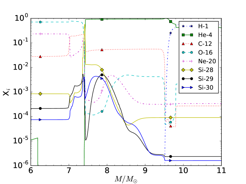
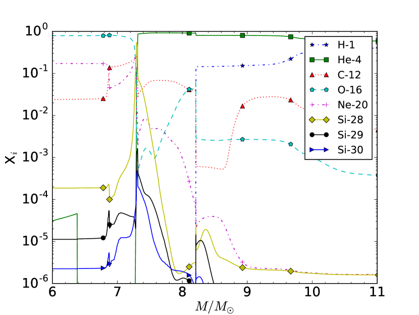
Figure 25: Abundance profiles of the C/Si zones after the passage of the SN shock for stellar models with $M_{\rm ZAMS}=25\,{\rm M}_{\odot}$ at $Z=0.006$ (top) and $Z=0.0001$ (bottom). Shown are the $\alpha$-chain isotope ${}^{\makebox[7.0pt][r]{$\scriptstyle 28$}}_{\makebox[7.0pt][r]{$\scriptstyle$}}\mathrm{Si}$ and the n-process isotopes ${}^{\makebox[17.61107pt][r]{$\scriptstyle 29,30$}}_{\makebox[17.61107pt][r]{$\scriptstyle$}}\mathrm{Si}$.

The C/Si zone in the stellar models with higher metallicity is more extended as shown in the comparison of the stellar models with $M_{\rm ZAMS}=25\,{\rm M}_{\odot}$ at $Z=0.006$ and $Z=0.0001$ in Fig. 25. As discussed in Pignatari et al. (2013b), $\alpha$-captures on ${}^{\makebox[7.0pt][r]{$\scriptstyle 16$}}_{\makebox[7.0pt][r]{$\scriptstyle$}}\mathrm{O}$ and ${}^{\makebox[7.0pt][r]{$\scriptstyle 20$}}_{\makebox[7.0pt][r]{$\scriptstyle$}}\mathrm{Ne}$ are in competition with the nucleosynthesis channel (n,$\gamma$)($\alpha$,n), leading to the production of the same species as the ($\alpha$,$\gamma$) reactions. The ($\alpha$,p) reactions are in balance with their reverse reactions. As a consequence, the nucleosynthesis in the C/Si zone is not much affected by metallicity and the observed C/Si zone size is due to the metallicity-dependence of the pre-SN evolution and the SN shock temperature.

Neutron-rich isotopes are produced via the neutron source ${}^{\makebox[7.0pt][r]{$\scriptstyle 22$}}_{\makebox[7.0pt][r]{$\scriptstyle$}}\mathrm{Ne}$($\alpha$,n)${}^{\makebox[7.0pt][r]{$\scriptstyle 25$}}_{\makebox[7.0pt][r]{$\scriptstyle$}}\mathrm{Mg}$ of the n process in the He/C zone of the He shell during the explosive nucleosynthesis of massive star models (Thielemann et al., 1979; Meyer et al., 2000; Rauscher et al., 2002; Pignatari et al., 2017). As fallback in the most massive stellar models with $M_{\rm ZAMS}=25\,{\rm M}_{\odot}$ prevents the ejection of deeper layers the more externally located C/Si zone and n-process enriched He/C zone become more relevant for the total yields. In the $M_{\rm ZAMS}=25\,{\rm M}_{\odot}$, $Z=0.006$ stellar model the largest contribution to the n-rich ${}^{\makebox[7.0pt][r]{$\scriptstyle 40$}}_{\makebox[7.0pt][r]{$\scriptstyle$}}\mathrm{Ar}$ originates from the n process inside the C/Si zone. The efficiency of the n-process production decreases with metallicity as indicated in the decrease of the yields of its tracer ${}^{\makebox[7.0pt][r]{$\scriptstyle 30$}}_{\makebox[7.0pt][r]{$\scriptstyle$}}\mathrm{Si}$ (Fig. 25). This is due to the secondary nature of ${}^{\makebox[7.0pt][r]{$\scriptstyle 22$}}_{\makebox[7.0pt][r]{$\scriptstyle$}}\mathrm{Ne}$ which abundance is made by the initial CNO abundances (e.g. Peters, 1968).

4.4 Shell merger nucleosynthesis

During Si shell burning convective O-C shell mergers occur in the massive star models with $M_{\rm ZAMS}/\,{\rm M}_{\odot}$ = 12, 15, 20 at $Z=0.01$ and $M_{\rm ZAMS}=15\,{\rm M}_{\odot}$ at $Z=0.02$. In these models the convective O shell increases in mass and touches the C-shell. C-shell material is mixed into the O shell until both convective shells fully merge. Burning of the ingested Ne results in large overproduction factors of the odd-Z elements P, Cl, K and Sc in Fig. 21 (Ritter et al., 2017a). These shell merger may harbour significant additional production of p-process nuclei such as ${}^{\makebox[24.61107pt][r]{$\scriptstyle 130,132$}}_{\makebox[24.61107pt][r]{$\scriptstyle$}}\mathrm{Ba}$. The amount of p-process nuclei produced depends on initial mass and metallicity.

In the stellar model with initial mass of $20\,{\rm M}_{\odot}$ at $Z=0.01$ the convective Si burning shell grows in mass until it reaches the C shell. In the following merger of the convective Si-O shell and convective C shell Fe-peak elements are transported out of the deeper layers which fall back onto the remnant during CCSN. This boosts the production of Fe peak elements, in particular Cr and leads to large overproduction factors (Fig. 21). The overproduction factor of Cr of the $M_{\rm ZAMS}=25\,{\rm M}_{\odot}$, $Z=0.01$ model is more than $1.7\,\mathrm{dex}$ larger than found in other stellar models at the same metallicity and the Cr production in our stellar models is already too high compared to observations (Côté et al., 2017).

Stellar evolution simulations based on the mixing-length theory describe convection through time and spherically-symmetric averages. This approach can not describe the interaction of convective C, O and Si burning shells (Meakin & Arnett, 2006; Arnett & Meakin, 2011). Results from 1D stellar evolution are therefore mostly qualitative (Andrassy et al., in prep.). 3D hydrodynamic simulations are required to analyze in which situations O-C shell merger happen, and the dynamics of the convective shells when they happen (Ritter et al., 2017a).

4.5 Fe-peak elements

The nucleosynthesis of the Fe-peak elements with even number of protons in massive stars is primary, and therefore does not depend on the initial metallicity (e.g. Prantzos, 2000; Woosley et al., 2002). However, the supernova progenitor evolution and the amount of fallback do depend on the initial metallicity and hence the total yields of these primary Fe-peak elements depend in some cases strongly on the initial metallicity (Table 12 and online yield tables).

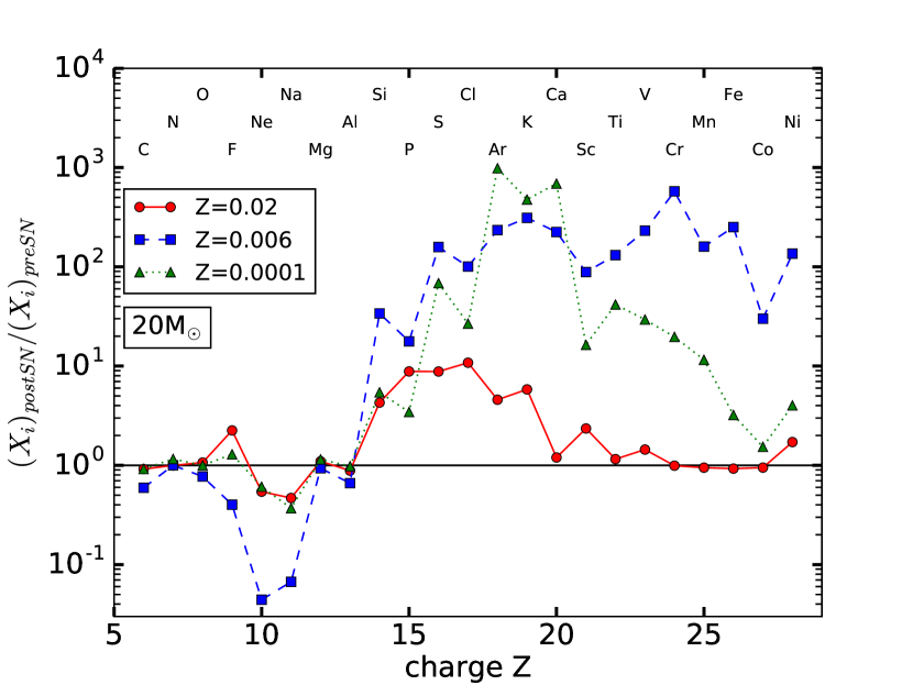
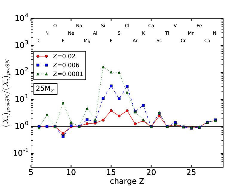
Figure 26: Ratio of SN to pre-SN yields versus charge number of stellar models with $M_{\rm ZAMS}=15$, $20$, $25\,{\rm M}_{\odot}$ for $Z=0.02$, $Z=0.006$ and $Z=0.0001$. The pre-SN yields are the ejected pre-SN composition above the mass cut (Sect. 2.3).

If not mentioned otherwise we discuss the delayed explosions (see Sect. 2.2). Fallback limits the ejection of Fe-peak elements which becomes important in $M_{\rm ZAMS}\geq 20\,{\rm M}_{\odot}$ models, but less so at lower initial mass. Fallback prevents any Fe ejection in stellar models with $M_{\rm ZAMS}=25\,{\rm M}_{\odot}$ which results in low overproduction factors of Fe (Fig. 21 to Fig. 23). In the stellar models with $M_{\rm ZAMS}=15\,{\rm M}_{\odot}$ the ratio of explosive production to pre-SN production (see pre-SN yield definition in Sect. 2.3) of Fe peak elements is much larger at $Z=0.0001$ compared to $Z=0.006$ due to a contribution of Fe-core layers to the pre-SN production at the latter metallicity (Fig. 26). This is due to a lower explosive Fe-peak production in stellar model of higher metallicity.

Of all stellar models with $M_{\rm ZAMS}=20\,{\rm M}_{\odot}$ only the $Z=0.006$ model produces Fe peak elements during SN shock nucleosynthesis. Consequently this model has the largest ratio of Fe peak elements produced during SN to the pre-SN production. In stellar models with $M_{\rm ZAMS}=12$ and $15\,{\rm M}_{\odot}$ additional production and ejection of Fe-peak elements originates from the $\alpha$-rich freeze-out layer which falls back in stellar models of higher initial mass (Sect. 4.7). The interplay of the core masses at collapse (Fig. 10) and the effect of fallback (Table 4) results in much larger variations of the Fe-peak elements ejection with initial mass and metallicity, compared to other yield sets for massive stars (e.g. Woosley & Weaver, 1995; Nomoto et al., 2006).

4.6 H-ingestion nucleosynthesis

While Li is produced through HBB in AGB models (Sect. 4.2) it is also effectively produced by H ingestion events (Sect. 3.2.1) in the second thermal pulse of the $1\,{\rm M}_{\odot}$, $Z=0.0001$ model and the post-AGB thermal pulse of the $1.0\,{\rm M}_{\odot}$, $Z=0.006$ model as decayed ${}^{\makebox[3.5pt][r]{$\scriptstyle 7$}}_{\makebox[3.5pt][r]{$\scriptstyle$}}\mathrm{Be}$ via ${}^{\makebox[3.5pt][r]{$\scriptstyle 3$}}_{\makebox[3.5pt][r]{$\scriptstyle$}}\mathrm{He}$($\alpha$,g)${}^{\makebox[3.5pt][r]{$\scriptstyle 7$}}_{\makebox[3.5pt][r]{$\scriptstyle$}}\mathrm{Be}$ where ${}^{\makebox[3.5pt][r]{$\scriptstyle 3$}}_{\makebox[3.5pt][r]{$\scriptstyle$}}\mathrm{He}$ is ingested with H (Herwig & Langer, 2001; Iwamoto et al., 2004). The post-AGB model production does not contribute to the yields as the enriched mass ejected into the interstellar medium is too small. The $Z=0.0001$ model loses ${}^{\makebox[3.5pt][r]{$\scriptstyle 7$}}_{\makebox[3.5pt][r]{$\scriptstyle$}}\mathrm{Li}$-enriched mass efficiently leading to large Li overproduction factors (Fig. 18).

H-ingestion events are also present in massive star models. They involve a ingestion of protons into the He-convection shell and reduce the He-core core mass by about $1\,{\rm M}_{\odot}$. The nucleosynthetic effect of H-ingestion events becomes apparent when the SN shock reaches the He shell which results in explosive He-burning with a small amount of added H. The exact amount and nature and amount of the H ingestion would depend on the 3D hydrodynamic nature of convection in such conditions.

H ingestion in massive stars (see Sect. 3.2.1) can lead to the production of ${}^{\makebox[3.5pt][r]{$\scriptstyle 7$}}_{\makebox[3.5pt][r]{$\scriptstyle$}}\mathrm{Be}$ during the explosion. H that reaches to the bottom of the He-shell just before the collapse produces ${}^{\makebox[3.5pt][r]{$\scriptstyle 3$}}_{\makebox[3.5pt][r]{$\scriptstyle$}}\mathrm{He}$ under explosive conditions and then ${}^{\makebox[3.5pt][r]{$\scriptstyle 7$}}_{\makebox[3.5pt][r]{$\scriptstyle$}}\mathrm{Be}$ via the reaction mentioned above. This ${}^{\makebox[3.5pt][r]{$\scriptstyle 7$}}_{\makebox[3.5pt][r]{$\scriptstyle$}}\mathrm{Be}$ would be ejected without the possibility to capture an electron to produce ${}^{\makebox[3.5pt][r]{$\scriptstyle 7$}}_{\makebox[3.5pt][r]{$\scriptstyle$}}\mathrm{Li}$, and thus SN with previous H ingestions would be ${}^{\makebox[3.5pt][r]{$\scriptstyle 7$}}_{\makebox[3.5pt][r]{$\scriptstyle$}}\mathrm{Be}$ producers. Other Li production might occur by $\nu$-induced production in CCSN or via galactic cosmic rays (e.g. Prantzos, 2012; Banerjee et al., 2013), which are both not considered in this work.

H-ingestion leads to significant production of light elements such as Li and N in the $20$ and $25\,{\rm M}_{\odot}$, $Z=0.0001$ models (Fig. 23). Fig. 26 shows that there is however no explosive contribution to N from the $20\,{\rm M}_{\odot}$, $Z=0.0001$ model, while the 25$\,{\rm M}_{\odot}$ explosion adds approximately the same amount of N compared to the the pre-SN evolution. N production has been seen in massive star models at low-metallicity previously (e.g. Woosley & Weaver, 1995; Ekström et al., 2008) and Pop III models (Heger & Woosley, 2010).

As previously reported by Pignatari et al. (2015), ${}^{\makebox[7.0pt][r]{$\scriptstyle 15$}}_{\makebox[7.0pt][r]{$\scriptstyle$}}\mathrm{N}$ is effectively produced in the region of pre-SN H ingestion during the explosive nucleosynthesis in our models. In the SN explosion ${}^{\makebox[7.0pt][r]{$\scriptstyle 15$}}_{\makebox[7.0pt][r]{$\scriptstyle$}}\mathrm{N}$ is relative to its pre-SN abundance orders of magnitude more produced than ${}^{\makebox[7.0pt][r]{$\scriptstyle 14$}}_{\makebox[7.0pt][r]{$\scriptstyle$}}\mathrm{N}$ as visible in the ratio of SN yields to pre-SN yields of the stellar model with $M_{\rm ZAMS}=20\,{\rm M}_{\odot}$ in Fig. 27. The ingestion events might be a relevant source of primary production of ${}^{\makebox[7.0pt][r]{$\scriptstyle 14$}}_{\makebox[7.0pt][r]{$\scriptstyle$}}\mathrm{N}$ and ${}^{\makebox[7.0pt][r]{$\scriptstyle 15$}}_{\makebox[7.0pt][r]{$\scriptstyle$}}\mathrm{N}$ at low metallicity in contrast to the pre-explosive production in rotating massive star models (e.g. Hirschi, 2007) which do not predict the low ${}^{\makebox[7.0pt][r]{$\scriptstyle 14$}}_{\makebox[7.0pt][r]{$\scriptstyle$}}\mathrm{N}$/${}^{\makebox[7.0pt][r]{$\scriptstyle 15$}}_{\makebox[7.0pt][r]{$\scriptstyle$}}\mathrm{N}$ ratio observed at high redshift and the isotopic ratio of the Sun (Pignatari et al., 2015). ${}^{\makebox[7.0pt][r]{$\scriptstyle 19$}}_{\makebox[7.0pt][r]{$\scriptstyle$}}\mathrm{F}$ is also produced efficiently through ${}^{\makebox[7.0pt][r]{$\scriptstyle 15$}}_{\makebox[7.0pt][r]{$\scriptstyle$}}\mathrm{N}$($\alpha$,$\gamma$)${}^{\makebox[7.0pt][r]{$\scriptstyle 19$}}_{\makebox[7.0pt][r]{$\scriptstyle$}}\mathrm{F}$ in these stellar explosion with $M_{\rm ZAMS}=25\,{\rm M}_{\odot}$ (Fig. 23).

During the first TP of the $M_{\rm ZAMS}=1\,{\rm M}_{\odot}$, $Z=0.0001$ model the PDCZ reaches into the radiative H-rich envelope and small amounts of H are ingested similar to H-ingestion events reported previously (e.g. Fujimoto et al., 2000; Cristallo et al., 2009, and references within). Most ingested H is absorbed by ${}^{\makebox[7.0pt][r]{$\scriptstyle 12$}}_{\makebox[7.0pt][r]{$\scriptstyle$}}\mathrm{C}$ to produce ${}^{\makebox[7.0pt][r]{$\scriptstyle 13$}}_{\makebox[7.0pt][r]{$\scriptstyle$}}\mathrm{C}$ which produces neutron densities $N_{n}\approx 10^{7}\,\mathrm{cm}^{-3}$ via the ${}^{\makebox[7.0pt][r]{$\scriptstyle 13$}}_{\makebox[7.0pt][r]{$\scriptstyle$}}\mathrm{C}$ ($\alpha$,n) neutron source and synthesizes heavy elements up to Pb. During the second TP the PDCZ reaches out into the convective envelope (Fig. 15) and large amounts of H are mixed into the PDCZ which leads to the convective-reactive production of ${}^{\makebox[7.0pt][r]{$\scriptstyle 13$}}_{\makebox[7.0pt][r]{$\scriptstyle$}}\mathrm{C}$ as in the $2\,{\rm M}_{\odot}$, ${\rm[Fe/H]}=-2.7$ model of Iwamoto et al. (2004). The energy generation due to proton burning leads to a split of the convective zone and its bottom part reaches a neutron density of $N_{n}\approx 5\times 10^{13}\,\mathrm{cm}^{-3}$ which leads to additional production of heavy elements with large overproduction factors (Fig. 20). The process of neutron release is as in Iwamoto et al. (2004). Iwamoto et al. (2004) and Cristallo et al. (2009) report higher neutron densities of $N_{n}\approx 10^{14}\,\mathrm{cm}^{-3}$ and $N_{n}\approx 10^{15}\,\mathrm{cm}^{-3}$ respectively. This is the heavy-element production through $i$ process which is poorly described in stellar evolution models. As discussed in Sect. 3.2.1 it has been shown by Herwig et al. (2011) and Herwig et al. (2014) that the convective-reactive $i$-process nucleosynthesis can not be modelled correctly by present versions of MLT based convective mixing in 1D stellar evolution simulations. We do therefore not make any effort to ensure numerical convergence of a demonstrably insufficient modeling approximation, and defer more reliable $i$ process predictions to a time when better modeling approaches have been developed for this particular regime found in our models.

4.7 $\mathbf{\alpha}$ process

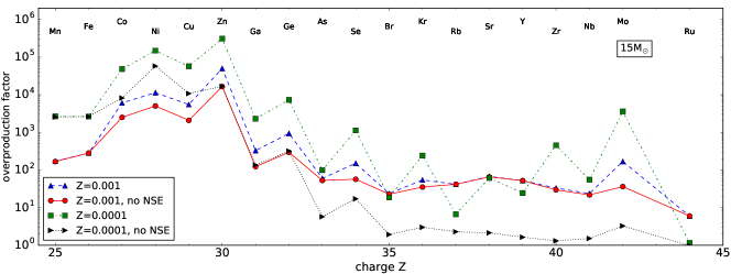
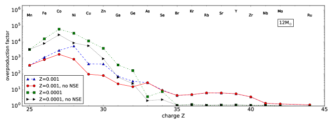
Figure 28: Overproduction factors versus charge number for stellar models with $M_{\rm ZAMS}=12\,{\rm M}_{\odot}$ and $M_{\rm ZAMS}=15\,{\rm M}_{\odot}$ at $Z=0.001$ and $Z=0.0001$ which reach $\alpha$-rich freeze out conditions during the CCSN explosion. Shown are the production factors of final yields under the assumption of fallback of the layers which went into NSE (no NSE). In the latter case layers which experience NSE conditions during the explosion were assumed not to be ejected.

Matter in nuclear statistical equilibrium (NSE) during the CCSN explosion which later on cools and expands can experience an $\alpha$-rich freeze-out (Woosley et al., 1973; Woosley & Hoffman, 1992). Such $\alpha$-rich freeze out conditions are reached in all our $M_{\rm ZAMS}=12\,{\rm M}_{\odot}$ and $M_{\rm ZAMS}=15\,{\rm M}_{\odot}$ models (Fig. 28). A larger $\alpha$-rich freeze-out layer formed during the explosive nucleosynthesis of the stellar models with $M_{\rm ZAMS}=15\,{\rm M}_{\odot}$ compared to the stellar models with $M_{\rm ZAMS}=12\,{\rm M}_{\odot}$ leads to a larger production of Fe-peak elements compared to the production in explosive Si burning. The $\alpha$-rich freeze out layers in the stellar models with $M_{\rm ZAMS}=15\,{\rm M}_{\odot}$ produce elements up to Mo in agreement with P16 (their Fig. 24). The massive star models of lower initial mass produce only elements up to Ge and Br at $Z=0.001$ and $Z=0.001$ respectively as indicated by their overproduction factors (Fig. 28). At lower metallicity heavier elements are produced in the NSE region than in stellar models of higher metallicity (Fig. 28).

4.8 Weak s process

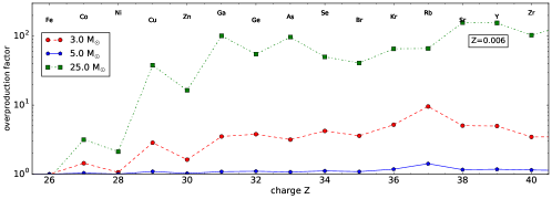
Figure 29: Comparison of overproduction factors versus charge of stellar models with $M_{\rm ZAMS}=3\,{\rm M}_{\odot}$ and $M_{\rm ZAMS}=5\,{\rm M}_{\odot}$ (main s-process) and of stellar models with $M_{\rm ZAMS}=25\,{\rm M}_{\odot}$ at $Z=0.006,0.001$ and $0.0001$ (weak s process).

The weak s process takes place at the end of core He-burning and during convective C shell burning in massive star models and is metallicity dependent. The process depends on the initial abundance of Fe seeds, and on the initial abundance of CNO nuclei that will make most of the ${}^{\makebox[7.0pt][r]{$\scriptstyle 22$}}_{\makebox[7.0pt][r]{$\scriptstyle$}}\mathrm{Ne}$ available as a neutron source (e.g. Käppeler et al., 1989; Prantzos et al., 1990; Raiteri et al., 1992; The et al., 2007; Pignatari et al., 2010; Käppeler et al., 2011; Frischknecht et al., 2016; Sukhbold et al., 2016). We compare the heavy element production up to the first s-process peak originating from the weak s process in these stellar models with $M_{\rm ZAMS}=25\,{\rm M}_{\odot}$ with element production from the main s process in these models with $M_{\rm ZAMS}=3\,{\rm M}_{\odot}$ and $M_{\rm ZAMS}=5\,{\rm M}_{\odot}$ for $Z=0.006$, $Z=0.001$ and $Z=0.0001$ in Fig. 29. The weak s-process efficiency is overall the largest at $Z=0.006$, also more than in models at higher metallicities. Because of the secondary nature of the weak s-process, this could appear as a surprising result. However, as already discussed in e.g. Pignatari & Gallino (2007), this is mostly due to the $\alpha$-enhancement on ${}^{\makebox[7.0pt][r]{$\scriptstyle 16$}}_{\makebox[7.0pt][r]{$\scriptstyle$}}\mathrm{O}$ at low metallicity, causing a smaller decrease of ${}^{\makebox[7.0pt][r]{$\scriptstyle 22$}}_{\makebox[7.0pt][r]{$\scriptstyle$}}\mathrm{Ne}$ with respect to the Fe seeds, that are instead decreasing linearly with the metallicity. As a consequence, the s-process distribution is also partially modified, showing a high production up to the Sr neutron-magic peak. For lower metallicities, also by taking into account $\alpha$-enhancement the resulting abundance of ${}^{\makebox[7.0pt][r]{$\scriptstyle 22$}}_{\makebox[7.0pt][r]{$\scriptstyle$}}\mathrm{Ne}$ becomes too low and the weak s-process contribution to the stellar yields becomes marginal. The fewer neutrons made by the ${}^{\makebox[7.0pt][r]{$\scriptstyle 22$}}_{\makebox[7.0pt][r]{$\scriptstyle$}}\mathrm{Ne}$($\alpha$,n)${}^{\makebox[7.0pt][r]{$\scriptstyle 25$}}_{\makebox[7.0pt][r]{$\scriptstyle$}}\mathrm{Mg}$ reaction are captured by primary neutron poisons like ${}^{\makebox[7.0pt][r]{$\scriptstyle 16$}}_{\makebox[7.0pt][r]{$\scriptstyle$}}\mathrm{O}$ (Baraffe et al., 1992; Pignatari & Gallino, 2007). The overproduction factors of elements above As even decrease in the massive star models at $Z=0.0001$ below those of the AGB models (Fig. 29).

The overproduction factors of the s-only isotopes ${}^{\makebox[7.0pt][r]{$\scriptstyle 70$}}_{\makebox[7.0pt][r]{$\scriptstyle$}}\mathrm{Ge}$, ${}^{\makebox[7.0pt][r]{$\scriptstyle 76$}}_{\makebox[7.0pt][r]{$\scriptstyle$}}\mathrm{Se}$, ${}^{\makebox[17.61107pt][r]{$\scriptstyle 80,82$}}_{\makebox[17.61107pt][r]{$\scriptstyle$}}\mathrm{Kr}$ and ${}^{\makebox[17.61107pt][r]{$\scriptstyle 86,87$}}_{\makebox[17.61107pt][r]{$\scriptstyle$}}\mathrm{Sr}$ of the stellar models with $M_{\rm ZAMS}=25\,{\rm M}_{\odot}$ at $Z=0.006$, $Z=0.001$ and $Z=0.0001$ show a decrease in the s-process efficiency below $Z=0.001$ (Fig. 30). Most production of ${}^{\makebox[7.0pt][r]{$\scriptstyle 70$}}_{\makebox[7.0pt][r]{$\scriptstyle$}}\mathrm{Ge}$ takes place in the pre-explosive nucleosynthesis as indicated by the overproduction factors of the pre-SN ejecta compared to the SN ejecta for the model at $Z=0.006$ (Fig. 30). In stellar models of lower initial mass the explosive nucleosynthesis produces further ${}^{\makebox[7.0pt][r]{$\scriptstyle 70$}}_{\makebox[7.0pt][r]{$\scriptstyle$}}\mathrm{Ge}$ which increases the overproduction factors of the SN ejecta over that of the pre-SN ejecta. The high production in the stellar model with $M_{\rm ZAMS}=15\,{\rm M}_{\odot}$ at $Z=0.006$ originates from a thin shocked Fe core layer.

4.9 Main s process

The main s process takes place in the ${}^{13}\mathrm{C}$-pocket of low-mass AGB stars and in much smaller amounts in the PDCZ of massive AGB stars. The s-process abundance distribution depends on the metallicity of the star, because of the combined effect of the primary neutron source ${}^{\makebox[7.0pt][r]{$\scriptstyle 13$}}_{\makebox[7.0pt][r]{$\scriptstyle$}}\mathrm{C}$ and of the secondary nature of the Fe seeds (Gallino et al., 1998; Busso et al., 1999). In these AGB models the ${}^{13}\mathrm{C}$-pocket size $M_{{}^{13}\mathrm{C}}$ depends on the efficiency of the CBM and decreases at $Z=0.0001$ from the $M_{{}^{13}\mathrm{C}}\approx 10^{-4}\,{\rm M}_{\odot}$ in the model with $M_{\rm ZAMS}=1.65\,{\rm M}_{\odot}$ to $M_{{}^{13}\mathrm{C}}\approx 10^{-8}\,{\rm M}_{\odot}$ in the model with $M_{\rm ZAMS}=7\,{\rm M}_{\odot}$ (Fig. 31). This is to a large extent due to the drastic reduction of $f_{\mathrm{\rm CE}}$ during the dredge-up in AGB stars with $M_{\rm ZAMS}\geq 4\,{\rm M}_{\odot}$ (Table 3). $M_{{}^{13}\mathrm{C}}$ in the 2$\,{\rm M}_{\odot}$ model is similar to $3.7\times 10^{-5}\,{\rm M}_{\odot}$ in stellar models at solar metallicity of Lugaro et al. (2003) and $2-3\times 10^{-5}\,{\rm M}_{\odot}$ in models at $Z=0.02$ in P16. The decreasing pocket size with initial mass leads to a drastic decrease of s-process production in massive AGB and S-AGB models.

We compare the overproduction factors of heavy elements of the low-mass AGB models, massive AGB models and S-AGB models with AGB models of $Z=0.02$ from P16 in Fig. 31. In stellar models with initial mass of $M_{\rm ZAMS}=1\,{\rm M}_{\odot}$ at $Z=0.006$ and $Z=0.001$ inefficient TDUP leads to little surface enrichment except for the model at $Z=0.0001$ which experiences H ingestion (Sect. 4.6). The total dredged-up mass $M_{D}$ of AGB models increases in initial mass up to $M_{\rm ZAMS}=2\,{\rm M}_{\odot}$ (Table 7) which leads to an increase of the overproduction factors of heavy elements with initial mass (Fig. 31). For larger initial masses the overproduction factors of peak s-process elements tend to decrease because of the larger envelope masses dilute the heavy elements, a decrease of $M_{D}$ and smaller ${}^{13}\mathrm{C}$ pockets.

With decreasing metallicity lower initial masses have the largest overproduction factors (Fig. 31). The largest overproduction factors of Sr and Pb are present in low-mass AGB models with initial masses below $4\,{\rm M}_{\odot}$. Rb is efficiently produced in the TP of massive AGB stars and its ratio to Sr, which is mostly produced in low-mass AGB models, increases from low-mass AGB stars to massive AGB stars (Fig. 31) in agreement with the observed high Rb/Sr ratio of massive AGB stars (e.g. García-Hernández et al., 2013). At lower metallicity the higher pulse temperature $T_{\rm PDCZ}$ results in a larger Rb/Sr ratio in the stellar models with $M_{\rm ZAMS}=2\,{\rm M}_{\odot}$ (Fig. 31).

${}^{\makebox[7.0pt][r]{$\scriptstyle 87$}}_{\makebox[7.0pt][r]{$\scriptstyle$}}\mathrm{Rb}$ and ${}^{\makebox[7.0pt][r]{$\scriptstyle 88$}}_{\makebox[7.0pt][r]{$\scriptstyle$}}\mathrm{Sr}$ have the largest overproduction factors of all AGB models at $Z=0.006$ in the $M_{\rm ZAMS}=4\,{\rm M}_{\odot}$, $Z=0.006$ model in agreement with models of the same initial mass at $Z=0.01$ of P16. ${}^{\makebox[10.5pt][r]{$\scriptstyle 208$}}_{\makebox[10.5pt][r]{$\scriptstyle$}}\mathrm{Pb}$ has the highest overproduction factor of all AGB models at $Z=0.006$ in the $M_{\rm ZAMS}=3\,{\rm M}_{\odot}$, $Z=0.006$ model in agreement with AGB models at $Z=0.01$ of P16. A comparison between these results and other models available in the literature is provided in Sect. 5.

4.10 $\gamma$ process

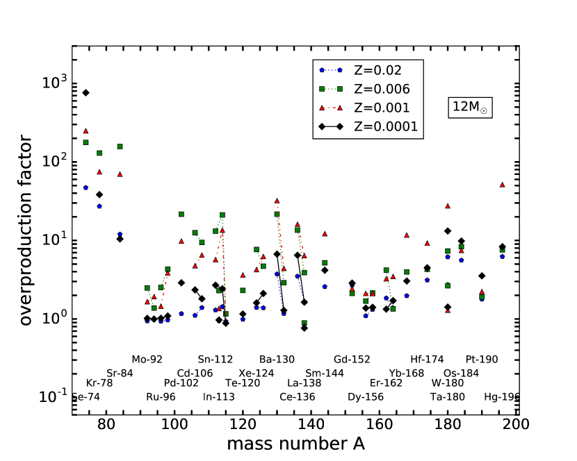
Figure 32: Overproduction factors versus mass number of p nuclei and their metallicity-dependence in massive star models with $M_{\rm ZAMS}=12\,{\rm M}_{\odot}$ (top) and $M_{\rm ZAMS}=20\,{\rm M}_{\odot}$ (bottom).

The $\gamma$ process produces proton-rich (p) nuclei in explosive Ne- and O-burning layers of CCSN models, where heavy seed nuclei are destroyed through photo-disintegration and proton capture (Woosley & Howard, 1978). For a review of the $\gamma$-process production and its uncertainties we refer to e.g. Arnould & Goriely (2003); Rauscher et al. (2013); Pignatari et al. (2016a); Rauscher et al. (2016). In the massive star models presented here, the lightest p-process nuclei ${}^{\makebox[7.0pt][r]{$\scriptstyle 74$}}_{\makebox[7.0pt][r]{$\scriptstyle$}}\mathrm{Se}$, ${}^{\makebox[7.0pt][r]{$\scriptstyle 78$}}_{\makebox[7.0pt][r]{$\scriptstyle$}}\mathrm{Kr}$ and ${}^{\makebox[7.0pt][r]{$\scriptstyle 84$}}_{\makebox[7.0pt][r]{$\scriptstyle$}}\mathrm{Sr}$ are more produced than most heavier $\gamma$-process isotopes in stellar models with initial mass up to $M_{\rm ZAMS}=20\,{\rm M}_{\odot}$ (Fig. 32). These isotopes are formed in the deepest layers of explosive O burning owing to their light masses and strong fallback prevents any production of ${}^{\makebox[7.0pt][r]{$\scriptstyle 74$}}_{\makebox[7.0pt][r]{$\scriptstyle$}}\mathrm{Se}$, ${}^{\makebox[7.0pt][r]{$\scriptstyle 78$}}_{\makebox[7.0pt][r]{$\scriptstyle$}}\mathrm{Kr}$ and ${}^{\makebox[7.0pt][r]{$\scriptstyle 84$}}_{\makebox[7.0pt][r]{$\scriptstyle$}}\mathrm{Sr}$ in the massive star models with $M_{\rm ZAMS}=25\,{\rm M}_{\odot}$. In the latter models only the heaviest p-process nuclei such as ${}^{\makebox[10.5pt][r]{$\scriptstyle 180$}}_{\makebox[10.5pt][r]{$\scriptstyle$}}\mathrm{Ta}$ and ${}^{\makebox[10.5pt][r]{$\scriptstyle 180$}}_{\makebox[10.5pt][r]{$\scriptstyle$}}\mathrm{W}$ are ejected.

Models with $M_{\rm ZAMS}=15\,{\rm M}_{\odot}$ produce the majority of $\gamma$-process isotopes from the $\alpha$-rich freeze-out layers. For increasing metallicity the relative contribution of the $\alpha$-rich freeze-out material to the total amount of produced ${}^{\makebox[7.0pt][r]{$\scriptstyle 74$}}_{\makebox[7.0pt][r]{$\scriptstyle$}}\mathrm{Se}$, ${}^{\makebox[7.0pt][r]{$\scriptstyle 78$}}_{\makebox[7.0pt][r]{$\scriptstyle$}}\mathrm{Kr}$ and ${}^{\makebox[7.0pt][r]{$\scriptstyle 84$}}_{\makebox[7.0pt][r]{$\scriptstyle$}}\mathrm{Sr}$ decreases. At $Z=0.006$ the production in $\alpha$-rich freeze-out layers of the stellar model with $M_{\rm ZAMS}=15\,{\rm M}_{\odot}$ would become negligible. But in this model an additional production of light p-process nuclei takes place in a shocked and ejected thin Fe core layer.

The dominant production of ${}^{\makebox[17.61107pt][r]{$\scriptstyle 92,94$}}_{\makebox[17.61107pt][r]{$\scriptstyle$}}\mathrm{Mo}$, including contributions to ${}^{\makebox[17.61107pt][r]{$\scriptstyle 96,98$}}_{\makebox[17.61107pt][r]{$\scriptstyle$}}\mathrm{Ru}$, occurs in the same $\alpha$-rich freeze-out layers as ${}^{\makebox[7.0pt][r]{$\scriptstyle 74$}}_{\makebox[7.0pt][r]{$\scriptstyle$}}\mathrm{Se}$, ${}^{\makebox[7.0pt][r]{$\scriptstyle 78$}}_{\makebox[7.0pt][r]{$\scriptstyle$}}\mathrm{Kr}$ and ${}^{\makebox[7.0pt][r]{$\scriptstyle 84$}}_{\makebox[7.0pt][r]{$\scriptstyle$}}\mathrm{Sr}$. Heavier $\gamma$-process isotopes are mostly produced in O and Ne shell burning of these massive star models. Both burning sites are the only $\gamma$-process sites in stellar models with $M_{\rm ZAMS}=20\,{\rm M}_{\odot}$ and $M_{\rm ZAMS}=25\,{\rm M}_{\odot}$ because of the lack of ejected $\alpha$-rich freeze-out layers. In stellar models with $M_{\rm ZAMS}=20\,{\rm M}_{\odot}$ we find larger overproduction factors than in those with $M_{\rm ZAMS}=12\,{\rm M}_{\odot}$ (Fig. 32). Nucleosynthesis in O-C shell mergers involves the $\gamma$ process (Sect. 4.4).

The $\gamma$-process production in massive stars is considered to be dominated by the SN explosive component (e.g. Arnould & Goriely, 2003, and references therein). However, in case of O-C shell mergers the pre-SN production is increased by orders of magnitudes, and it may become more relevant than the explosive $\gamma$-process component (Ritter et al., 2017a). In our stellar model set, the $M_{\rm ZAMS}=15\,{\rm M}_{\odot}$, $Z=0.02$ model and $M_{\rm ZAMS}=12\,{\rm M}_{\odot}$, $15\,{\rm M}_{\odot}$, and $20\,{\rm M}_{\odot}$ models at $Z=0.01$ include O-C shell mergers, and carry this anomalous pre-SN signature.

wind
species	$1\,{\rm M}_{\odot}$	$1.65\,{\rm M}_{\odot}$	$2\,{\rm M}_{\odot}$	$3\,{\rm M}_{\odot}$	$4\,{\rm M}_{\odot}$	$5\,{\rm M}_{\odot}$	$6\,{\rm M}_{\odot}$	$7\,{\rm M}_{\odot}$	$12\,{\rm M}_{\odot}$	$15\,{\rm M}_{\odot}$	$20\,{\rm M}_{\odot}$	$25\,{\rm M}_{\odot}$
C	8.708E-03	2.147E-02	2.356E-02	8.884E-03	1.988E-03	7.856E-04	2.937E-04	1.797E-03	4.031E-07	2.472E-07	2.913E-07	4.980E-07
N	7.763E-05	5.710E-05	3.870E-05	3.408E-05	1.019E-02	4.692E-03	2.360E-03	8.018E-03	4.301E-07	2.674E-07	2.471E-08	4.223E-08
O	1.835E-03	8.626E-03	9.952E-03	2.781E-03	4.080E-03	1.833E-04	2.239E-04	3.249E-03	2.939E-06	1.671E-06	1.721E-06	2.942E-06
F	3.522E-08	2.432E-06	2.565E-06	3.756E-08	7.060E-09	1.065E-09	6.403E-10	9.822E-09	2.166E-11	1.246E-11	1.304E-11	2.229E-11
Ne	1.487E-05	8.758E-04	9.089E-04	1.138E-04	2.528E-04	4.369E-05	5.373E-05	1.268E-04	2.461E-07	1.412E-07	1.371E-07	2.344E-07
Na	1.903E-07	6.951E-06	6.375E-06	1.020E-06	1.500E-06	3.222E-07	1.138E-07	5.084E-07	8.330E-09	4.204E-09	9.296E-10	1.589E-09
Mg	1.005E-06	5.403E-05	9.078E-05	3.960E-05	1.193E-04	2.429E-05	1.937E-05	4.907E-05	7.500E-08	4.634E-08	3.896E-08	6.660E-08
Al	3.506E-08	3.905E-07	8.674E-07	6.366E-07	2.057E-06	2.275E-06	1.841E-06	1.037E-06	3.202E-09	1.937E-09	1.506E-09	2.575E-09
Si	7.645E-07	1.791E-06	2.559E-06	3.970E-06	6.714E-06	7.136E-06	1.495E-05	9.418E-06	6.802E-08	3.953E-08	3.666E-08	6.266E-08
S	5.121E-07	1.134E-06	1.469E-06	2.391E-06	3.455E-06	4.471E-06	5.436E-06	6.386E-06	4.806E-08	2.793E-08	2.590E-08	4.427E-08
Ar	8.228E-08	1.820E-07	2.359E-07	3.843E-07	5.537E-07	7.182E-07	8.738E-07	1.027E-06	7.738E-09	4.498E-09	4.170E-09	7.129E-09
Ca	5.590E-08	1.240E-07	1.607E-07	2.630E-07	3.790E-07	4.920E-07	5.993E-07	7.038E-07	5.303E-09	3.082E-09	2.858E-09	4.885E-09
Fe	6.453E-07	1.451E-06	1.881E-06	3.073E-06	4.429E-06	5.754E-06	7.012E-06	8.238E-06	6.202E-08	3.605E-08	3.342E-08	5.714E-08
Sr	6.005E-09	3.708E-09	2.515E-09	1.657E-09	2.446E-09	1.014E-09	3.665E-10	3.752E-10	2.619E-12	1.522E-12	1.411E-12	2.412E-12
Ba	3.250E-09	2.820E-10	2.351E-10	4.156E-10	9.354E-10	2.492E-10	9.297E-11	1.114E-10	7.818E-13	4.544E-13	4.213E-13	7.202E-13
Eu	3.857E-12	6.504E-13	9.461E-13	1.386E-12	2.736E-12	1.848E-12	1.967E-12	2.290E-12	1.849E-14	1.075E-14	9.967E-15	1.704E-14
Pb	3.221E-10	4.503E-10	7.906E-10	2.868E-10	5.420E-10	2.010E-10	8.544E-11	9.068E-11	6.482E-13	3.768E-13	3.493E-13	5.972E-13

wind + pre-SN ejecta
species	$12\,{\rm M}_{\odot}$	$15\,{\rm M}_{\odot}$	$20\,{\rm M}_{\odot}$	$25\,{\rm M}_{\odot}$
C	1.294E-01	1.686E-01	2.128E-01	2.320E-01
N	2.159E-04	3.034E-04	2.001E-02	1.041E-02
O	7.383E-01	1.339E+00	2.044E+00	7.407E-01
F	2.482E-08	3.120E-08	7.212E-08	3.463E-07
Ne	6.624E-02	1.989E-01	2.638E-01	8.609E-02
Na	2.475E-04	8.799E-04	1.662E-03	1.031E-03
Mg	6.435E-02	7.448E-02	1.011E-01	4.728E-03
Al	1.640E-03	1.436E-03	1.536E-03	7.644E-05
Si	4.380E-02	1.183E-01	2.093E-02	1.294E-04
S	6.015E-03	7.430E-02	4.377E-04	2.055E-05
Ar	3.365E-04	8.531E-03	3.551E-06	3.270E-06
Ca	3.565E-06	3.916E-05	1.977E-06	2.233E-06
Fe	1.204E-02	3.753E-05	2.378E-05	2.648E-05
Sr	9.471E-10	1.915E-09	3.577E-09	2.253E-09
Ba	2.181E-10	3.039E-10	4.202E-10	3.869E-10
Eu	3.695E-12	4.508E-12	5.702E-12	6.867E-12
Pb	1.697E-10	2.311E-10	3.149E-10	3.012E-10

Wind + SN ejecta
$12\,{\rm M}_{\odot}$	$15\,{\rm M}_{\odot}$	$20\,{\rm M}_{\odot}$	$25\,{\rm M}_{\odot}$
1.226E-01	1.646E-01	1.956E-01	2.037E-01
2.164E-04	3.050E-04	2.320E-02	2.813E-02
2.828E-01	1.176E+00	2.043E+00	7.062E-01
2.752E-08	4.500E-08	9.317E-08	2.585E-06
6.669E-03	1.469E-01	1.607E-01	1.227E-01
1.812E-05	5.359E-04	6.145E-04	1.018E-03
1.638E-02	7.562E-02	1.160E-01	2.178E-02
6.219E-05	1.157E-03	1.505E-03	1.315E-04
9.289E-02	1.078E-01	1.138E-01	2.063E-02
5.446E-02	4.459E-02	2.999E-02	2.046E-03
1.083E-02	7.684E-03	3.495E-03	1.122E-05
8.686E-03	5.152E-03	1.363E-03	2.159E-06
2.443E-01	5.073E-02	7.649E-05	2.524E-05
7.219E-10	4.976E-08	3.417E-09	2.215E-09
1.771E-10	2.812E-10	3.836E-10	3.739E-10
3.874E-12	4.845E-12	5.932E-12	7.541E-12
1.450E-10	2.163E-10	2.869E-10	3.093E-10

Table 12: Yields derived from stellar winds, pre-SN and SN ejecta for $Z=0.0001$. The SN ejecta is produced with the delayed explosion prescription. We provide tables for other metallicities online (Appendix A).

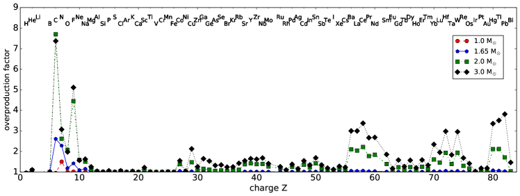
Figure 17: Overproduction factors versus charge number of final yields of AGB models at $Z=0.01$ with stellar models of $M_{\rm ZAMS}/\,{\rm M}_{\odot}$ = 1.65, 2, 3, 4, 5 of P16.

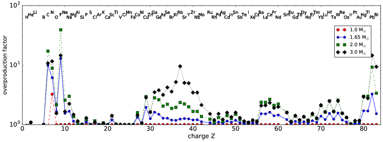
Figure 18: Overproduction factors versus charge number of final yields of AGB models at $Z=0.006$.

Figure 19: Overproduction factors versus charge number of final yields of AGB models at $Z=0.001$.

Figure 20: Overproduction factors versus charge number of final yields of AGB models at $Z=0.0001$.

Figure 21: Overproduction factors of final yields massive star models at $Z=0.02$ (top) and $Z=0.01$ (bottom).

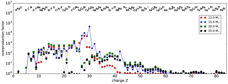
Figure 22: Overproduction factors versus charge number of massive star models at $Z=0.006$ (top) and $Z=0.001$ (bottom).

Figure 23: Overproduction factors versus charge number of final yields of massive star models at $Z=0.0001$.

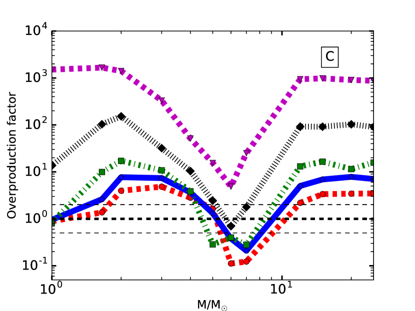
Figure 24: Overproduction factors of CNO isotopes versus initial mass of final yields. The dashed horizontal lines indicate the values 0.5, 1 and 2. Plots for all stable elements and many isotopes at all metallicities presented in this work are available online at http://nugridstars.org/data-and-software/yields/set-1.

Figure 27: Ratio of SN to pre-SN yields versus mass number of stellar models with $M_{\rm ZAMS}=20\,{\rm M}_{\odot}$ for $Z=0.02$, $Z=0.006$ and $Z=0.0001$. The pre-SN yields are the ejected pre-SN composition above the mass cut (Sect. 2.3).

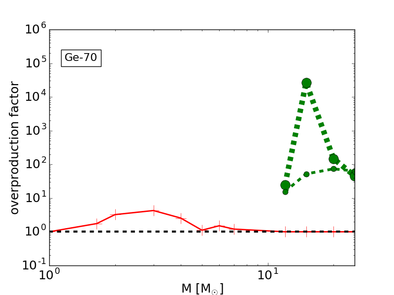
Figure 30: Overproduction factors versus mass number of final yields of stars with $M_{\rm ZAMS}=25\,{\rm M}_{\odot}$ at $Z=0.006$, $Z=0.001$ and $Z=0.0001$ with focus on the weak s-only isotopes ${}^{\makebox[7.0pt][r]{$\scriptstyle 70$}}_{\makebox[7.0pt][r]{$\scriptstyle$}}\mathrm{Ge}$, ${}^{\makebox[7.0pt][r]{$\scriptstyle 76$}}_{\makebox[7.0pt][r]{$\scriptstyle$}}\mathrm{Se}$,${}^{\makebox[17.61107pt][r]{$\scriptstyle 80,82$}}_{\makebox[17.61107pt][r]{$\scriptstyle$}}\mathrm{Kr}$ and ${}^{\makebox[17.61107pt][r]{$\scriptstyle 86,87$}}_{\makebox[17.61107pt][r]{$\scriptstyle$}}\mathrm{Sr}$ (top). The overproduction factors versus initial mass of ${}^{\makebox[7.0pt][r]{$\scriptstyle 70$}}_{\makebox[7.0pt][r]{$\scriptstyle$}}\mathrm{Ge}$ at $Z=0.006$ for stellar wind ejecta (solid line), pre-explosive ejecta (small circles) and explosive ejecta (large circles) with delayed explosion prescription (bottom). Plots for all stable elements and many isotopes at all metallicities including delayed and rapid explosion prescriptions are available online at http://nugridstars.org/data-and-software/yields/set-1.

Figure 31: Overproduction factors of heavy elements versus charge number of low-mass, massive and SAGB models. Included are AGB models at $Z=0.02$ of P16.

5 Discussion

In this section we first address model limitations arising from the choice of resolution in AGB models and massive star models. Afterwards, the resulting stellar yields of AGB models and massive star models are compared with previous works.

5.1 Resolution of AGB models

In AGB models the H and He shells become hotter and thinner with increasing initial mass and decreasing metallicity. This makes it challenging to model the bottom of the convective envelope and its boundary in massive AGB stars and S-AGB stars (Siess, 2010). To model the effect of HDUP (see Sect. 2.1.4) a high temporal and spatial resolution is required at the bottom of the convective envelope.

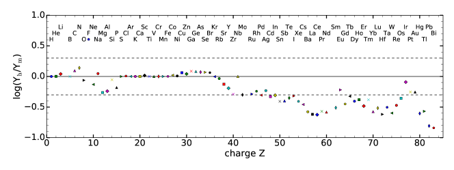
Figure 33: Ratio of final yields versus charge number based on a medium resolution ($Y_{m}$) and a high resolution ($Y_{h}$) of the $M_{\rm ZAMS}=4\,{\rm M}_{\odot}$, $Z=0.0001$ model. The dashed lines indicate a factor of 0.5 and 2.

To assess the sensitivity of resolution on the final yields a $M_{\rm ZAMS}=4$, $Z=0.0001$ model was calculated with increased resolution at the bottom boundary of the convective envelope and at the location of the ${}^{13}\mathrm{C}$ pocket. We compare this high-resolution calculation with up to $1.8\times 10^{4}$ zones with the calculation with moderate resolution of below $2\times 10^{3}$ zones. The latter resolution is similar to the resolution of the stellar models for which yields are calculated. No efforts have been made to reach convergence based on the resolution. Among light elements the biggest difference is in F which is overproduced by factor four. Mg and Al that are underproduced by less than a factor of two in the high-resolution runs compared to the lower-resolution run. Furthermore, the lower-resolution model produces two times as many elements at $Z\approx 50$ than the high-resolution model. For most elements beyond $Z\approx 50$ this production relative to the high-resolution model increases with a maximum of 6.7 for Bi and Pb (Fig. 33).

In order to resolve the ${}^{13}\mathrm{C}$ pocket down to the size of $M_{{}^{13}\mathrm{C}}\approx 10^{-8}\,{\rm M}_{\odot}$ that would be found, for example, in the 7$\,{\rm M}_{\odot}$ models owing to the decreased CBM efficiency $f_{\mathrm{CE}}$ in the most massive S-AGB models further resolution refinement below the convective boundary would be necessary. However, this is not required because at this level the ${}^{13}\mathrm{C}$ pocket does not contribute significantly to the $s$-process production of the more massive low-resolution AGB models.

The heavy element production in the ${}^{13}\mathrm{C}$ pocket for stellar models with $M_{\rm ZAMS}\geq 4\,{\rm M}_{\odot}$ decreases strongly due to a rapidly decreasing ${}^{13}\mathrm{C}$-pocket size (Fig. 18 to Fig. 20). For all AGB models with $M_{\rm ZAMS}>3\,{\rm M}_{\odot}$ we find $T_{\rm PDCZ}>3\times 10^{8}\,\mathrm{K}$ (Table 7) which is high enough to activate efficiently the ${}^{\makebox[7.0pt][r]{$\scriptstyle 22$}}_{\makebox[7.0pt][r]{$\scriptstyle$}}\mathrm{Ne}$($\alpha$,n)${}^{\makebox[7.0pt][r]{$\scriptstyle 25$}}_{\makebox[7.0pt][r]{$\scriptstyle$}}\mathrm{Mg}$ reaction. In these stellar models with $M_{\rm ZAMS}>4\,{\rm M}_{\odot}$ the PDCZ becomes the main production site of first-peak s-process elements (Fig. 18 to Fig. 20). The impact of the ${}^{13}\mathrm{C}$-pocket resolution on the yields of s-process elements in these stellar models is low. The influence of the resolution on the bottom boundary is not relevant for the chemical imprint of the AGB models with $M_{\rm ZAMS}>4\,{\rm M}_{\odot}$ and for GCE because there is no relevant element production in the ${}^{13}\mathrm{C}$ pocket. F is strongly affected by the resolution but is only produced in small amounts compared to AGB models of lower initial mass. We have therefore not improved the resolution for these models.

5.2 Resolution of massive star models

In these models the C/O ratio from the post-processing at the end of the core He-burning differs from the stellar evolution calculations by a factor of $\approx 30\,\%$ at $Z=0.02$ and $\approx$ 50  % at $Z=0.0001$. This discrepancy can be reduced in future calculations by reducing the time step, as done in Jones et al. (2015). The largest absolute differences are found at $Z=0.02$ because the the C/O ratio decreases with metallicity.

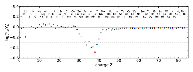
Figure 34: Ratios of yields versus charge number based on the $15\,{\rm M}_{\odot}$, $Z=0.02$ models computed with highly resolved core He-burning ($Y_{h}$) and with the default resolution ($Y_{l}$). The dashed line indicates a factor of 0.5.

The weak s-process at the end of core He-burning depends on the He-burning conditions for which the the ratio of the He-burning products C and O is an indicator. To analyze the impact of the C/O ratio difference on the weak s process we have selected a $M_{\rm ZAMS}=15\,{\rm M}_{\odot}$, $Z=0.02$ model which shows stronger s-process production compared to stars at lower metallicity. Using a sub-time stepping method we generate a resolved post-processing simulation that fully agrees with the stellar evolution simulation in the He-core C/O ratios. First-peak s-process element yields are lower by up to a factor of three in the the converged post-processed model compared to the lower-resolution model. (Fig. 34). These differences in final yields is within the uncertainty which results from the method which is applied to artificially explode the models: the difference between delay and rapid explosion prescription. The difference in yields between the resolved and lower-resolution models will impact GCE simulation only to the extent that the elements have a significant weak s-process contribution. In particular, this needs to be taken into account for the GCE of Cu, Ga and Ge (Pignatari et al., 2010).

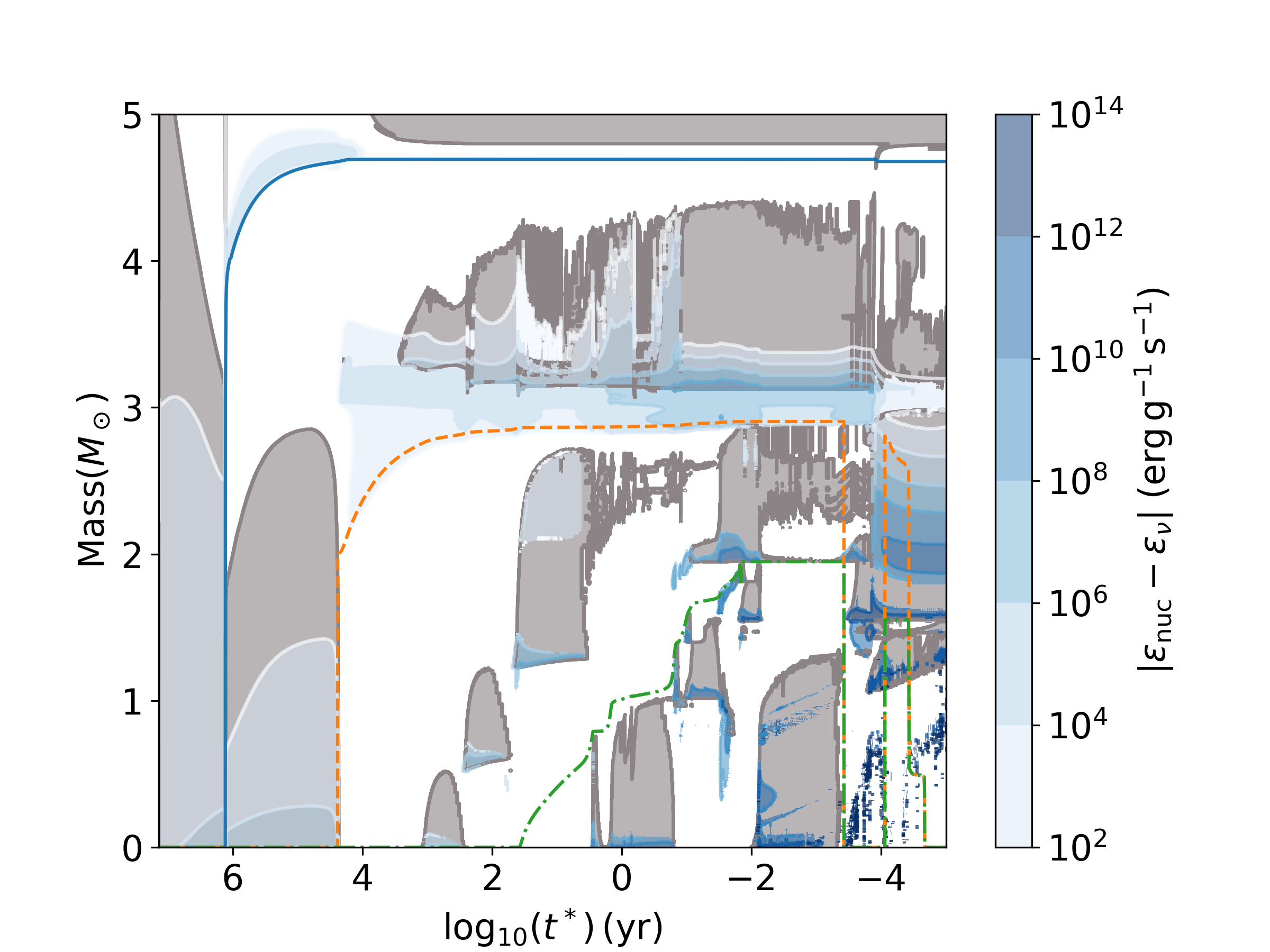
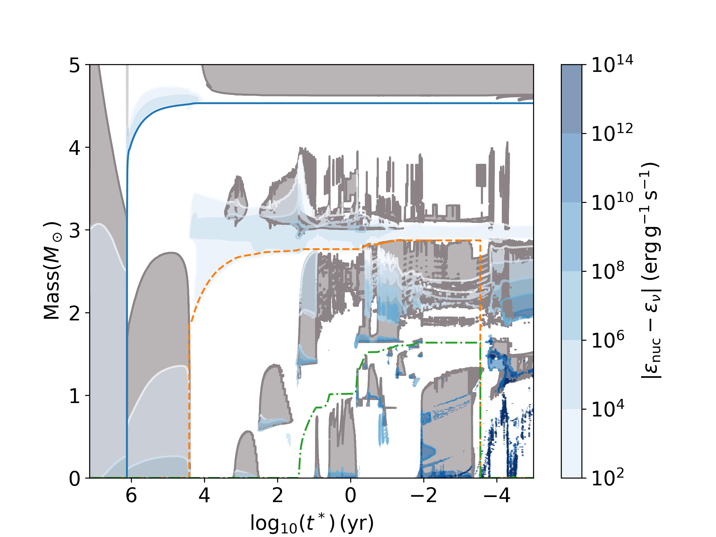
Figure 35: Kippenhahn diagrams as in Fig. 11 of two $M_{\rm ZAMS}=15\,{\rm M}_{\odot}$, $Z=0.02$ models with the default resolution (top) and with an increased resolution during core He-burning (bottom).

To analyze the effect of resolution on the stellar evolution simulation of massive stars we calculate a $M_{\rm ZAMS}=15\,{\rm M}_{\odot}$, $Z=0.02$ model with a factor between about two and ten higher time resolution of the He core-burning phase compared to the default-resolution model. We find that the He core is slightly smaller at higher resolution (Fig. 35). A major O-C shell merger which is present in the default-resolution model disappears at higher resolution. The occurrence of O-C shell mergers is ultimately dependent on the 3D hydrodynamic properties of of convection and CBM in the late stages of massive star models, which require multi-D hydrodynamic simulations (Meakin & Arnett, 2006; Herwig et al., 2014; Jones et al., 2017, Andrassy et al., in preparation). Numerical resolution of massive star models adds to the numerous other sources of uncertainty (Petermann et al., in preparation), and we plan to reduce this error in future updates of theses data sets.

5.3 Comparison with stellar yields in literature

5.3.1 AGB models

Yield sets of of AGB and S-AGB models have been presented by Karakas (2010), Siess (2010), the FRUITY database (Cristallo et al., 2011; Cristallo et al., 2015), Lugaro et al. (2012), Ventura et al. (2013), Fishlock et al. (2014), Doherty et al. (2014) and Karakas & Lugaro (2016). Others have published AGB and massive star yields such as the Padova group (Portinari et al., 1998; Marigo, 2001).

Low-mass AGB models

We compare yields of the $M_{\rm ZAMS}=2\,{\rm M}_{\odot}$, $Z=0.0001$ model of this work with yields of models of the same initial mass and metallicity from Herwig (2004a), Karakas (2010) and Straniero et al. (2014, S14) in Table 13. For the isotopes ${}^{\makebox[7.0pt][r]{$\scriptstyle 12$}}_{\makebox[7.0pt][r]{$\scriptstyle$}}\mathrm{C}$ and ${}^{\makebox[7.0pt][r]{$\scriptstyle 14$}}_{\makebox[7.0pt][r]{$\scriptstyle$}}\mathrm{N}$ we find yields in-between those of K10 and S14 and within a factor two of those of H04. The larger production of ${}^{\makebox[7.0pt][r]{$\scriptstyle 16$}}_{\makebox[7.0pt][r]{$\scriptstyle$}}\mathrm{O}$ compared to K10 and S14 is due to the choice of the CBM applied in the He intershell (Herwig, 2005). H04 get about 2.5 times lower O yield with the application of the same CBM efficiency. In this work s-process isotopes are less produced than in S14. The yield of ${}^{\makebox[7.0pt][r]{$\scriptstyle 88$}}_{\makebox[7.0pt][r]{$\scriptstyle$}}\mathrm{Sr}$ from the AGB model of this work is roughly 50% lower than of S14. The yields of ${}^{\makebox[10.5pt][r]{$\scriptstyle 138$}}_{\makebox[10.5pt][r]{$\scriptstyle$}}\mathrm{Ba}$ and ${}^{\makebox[10.5pt][r]{$\scriptstyle 208$}}_{\makebox[10.5pt][r]{$\scriptstyle$}}\mathrm{Pb}$ are by more than $1\,\mathrm{dex}$ and $2\,\mathrm{dex}$ lower than those of S14, respectively. We attribute the differences to less convective boundary mixing and smaller ${}^{13}\mathrm{C}$ pockets than in S14. The small ${}^{13}\mathrm{C}$ pocket sizes of these models correspond to lower [hs/ls] abundances of the observed s-process spread of C stars (see P16, Sect. 4.9). An updated model of ${}^{13}\mathrm{C}$-pocket formation through CBM induced by gravity waves has been recently proposed by Battino et al. (2016). It is able to explain the larger observed neutron-exposure signatures. The physics process that causes the spread of observed s-process is still matter of debate (e.g. Iben & Renzini, 1982; Herwig et al., 1997; Cristallo et al., 2001; Denissenkov & Tout, 2003; Herwig, 2005; Busso et al., 2007; Denissenkov et al., 2009; Battino et al., 2016; Trippella et al., 2016).

Massive AGB models

Yields of the $M_{\rm ZAMS}=5\,{\rm M}_{\odot}$, $Z=0.0001$ model of this work and yields from models of the same initial mass and metallicity from H04, K10 and C15 are shown in Table 14. The same trends as in the discussion on the nested-network for HBB can be observed here (Sect. 2.3). Differences between the yields from this work, H04 and K10 are similar within a factor 2-3, while showing the same trends in isotopic ratios. Our $M_{\rm ZAMS}=5\,{\rm M}_{\odot}$, $Z=0.0001$ model has lower s-process yields than our $M_{\rm ZAMS}=2\,{\rm M}_{\odot}$, $Z=0.0001$ model, because of the HDUP limit to the mixing at the bottom of the convective envelope CBM parameter (Sect. 3.2.3, Sect. 2.1.4) which leads to a lower ${}^{13}\mathrm{C}$ pocket contribution. The $M_{\rm ZAMS}=5\,{\rm M}_{\odot}$ s-process yields from this work are more than $1\,\mathrm{dex}$ below those of C15, which is due to the difference of CBM assumptions in these models.

5.3.2 Massive star models

Groups have published massive star yields at various metallicities, among others Woosley & Weaver (1995), the Geneva group (Hirschi et al., 2005; Frischknecht et al., 2016), Chieffi & Limongi (2004), Heger & Woosley (2010) and P16. We choose the yields of P16, Chieffi & Limongi (2004, CL04) and Kobayashi et al. (2006, K06) for a comparison with models of the same initial mass and metallicity of this work.

The metallicity dependence of the mass loss has a significant impact on the final yields. K06 apply a metallicity-dependent mass loss while CL04 do not include any mass loss. The total mass lost is $0.13\,{\rm M}_{\odot}$ and $0.41\,{\rm M}_{\odot}$ for the $M_{\rm ZAMS}=15\,{\rm M}_{\odot}$ model and the $M_{\rm ZAMS}=25\,{\rm M}_{\odot}$ model at $Z=0.001$ while K06 finds $0.08\,{\rm M}_{\odot}$ and $0.58\,{\rm M}_{\odot}$. The reduced mass loss at lower metallicity results in larger core masses when considering a similar mass cut and hence the ejection of larger amounts of O compared to models at higher metallicity.

Yields of the $M_{\rm ZAMS}=15\,{\rm M}_{\odot}$, $Z=0.02$ model of this work are compared with yields of the same initial mass and metallicity based on the models of P16 in Table 15. The yields of ${}^{\makebox[7.0pt][r]{$\scriptstyle 12$}}_{\makebox[7.0pt][r]{$\scriptstyle$}}\mathrm{C}$ and ${}^{\makebox[7.0pt][r]{$\scriptstyle 14$}}_{\makebox[7.0pt][r]{$\scriptstyle$}}\mathrm{N}$ are close to those of P16 while ${}^{\makebox[7.0pt][r]{$\scriptstyle 16$}}_{\makebox[7.0pt][r]{$\scriptstyle$}}\mathrm{O}$ yields are by about a factor three larger than in P16. We find only low sensitivity of the yields on the amount of fallback. For ${}^{\makebox[7.0pt][r]{$\scriptstyle 56$}}_{\makebox[7.0pt][r]{$\scriptstyle$}}\mathrm{Fe}$ the difference in yields to P16 increases and we find a factor of 3.2 and 4.5 lower Fe yields than in P16 because of less production of Fe in the explosion. ${}^{\makebox[7.0pt][r]{$\scriptstyle 88$}}_{\makebox[7.0pt][r]{$\scriptstyle$}}\mathrm{Sr}$ yields are more sensitive to the amount of fallback than the CNO species as in P16. ${}^{\makebox[7.0pt][r]{$\scriptstyle 88$}}_{\makebox[7.0pt][r]{$\scriptstyle$}}\mathrm{Sr}$ yield based on the delayed explosion prescription are by about a factor two larger than those of P16 which is within the expected difference due to the under-resolved He burning (Sect. 5.2).

At low metallicity we show yields of the $M_{\rm ZAMS}=15\,{\rm M}_{\odot}$, $Z=0.001$ model of this work and models of the same initial mass and metallicity by CL04 and K06 in Table 16. Yields of ${}^{\makebox[7.0pt][r]{$\scriptstyle 12$}}_{\makebox[7.0pt][r]{$\scriptstyle$}}\mathrm{C}$ and ${}^{\makebox[7.0pt][r]{$\scriptstyle 14$}}_{\makebox[7.0pt][r]{$\scriptstyle$}}\mathrm{N}$ are in between those of CL04 and K06 while ${}^{\makebox[7.0pt][r]{$\scriptstyle 16$}}_{\makebox[7.0pt][r]{$\scriptstyle$}}\mathrm{O}$ yields are larger than both works and roughly a factor of two larger than those of CL04. The range of ${}^{\makebox[7.0pt][r]{$\scriptstyle 56$}}_{\makebox[7.0pt][r]{$\scriptstyle$}}\mathrm{Fe}$ yields given through the delayed and rapid explosion prescriptions includes the yields of CL04 and K06. In contrast to this work CL04 and K06 fix the ejecta of Ni and Fe respectively and then adjust the amount of fallback. The yields of ${}^{\makebox[7.0pt][r]{$\scriptstyle 88$}}_{\makebox[7.0pt][r]{$\scriptstyle$}}\mathrm{Sr}$ in these massive star models are considerably larger than found in K06. Little fallback due to the rapid explosion prescription leads to about $3\,\mathrm{dex}$ more production of ${}^{\makebox[7.0pt][r]{$\scriptstyle 88$}}_{\makebox[7.0pt][r]{$\scriptstyle$}}\mathrm{Sr}$ compared to CL04, K06 and the corresponding model in our set calculated using the delay prescription. Most of the large production of ${}^{\makebox[7.0pt][r]{$\scriptstyle 88$}}_{\makebox[7.0pt][r]{$\scriptstyle$}}\mathrm{Sr}$ shown in Table 16 originates from the innermost $\sim$ 0.1M_⊙ layers, due to the activation of the $\alpha$-rich freeze out.

We compare yields of the $M_{\rm ZAMS}=25\,{\rm M}_{\odot}$, $Z=0.001$ model of this work with yields of models of the same initial mass and metallicity from CL04 and K06 in Table 17. ${}^{\makebox[7.0pt][r]{$\scriptstyle 12$}}_{\makebox[7.0pt][r]{$\scriptstyle$}}\mathrm{C}$ yields agree well with K06 yields and ${}^{\makebox[7.0pt][r]{$\scriptstyle 14$}}_{\makebox[7.0pt][r]{$\scriptstyle$}}\mathrm{N}$ yields with CL04 yields. We find lower ${}^{\makebox[7.0pt][r]{$\scriptstyle 16$}}_{\makebox[7.0pt][r]{$\scriptstyle$}}\mathrm{O}$ yields than CL04 and K06 which might be due to the fallback of larger parts of the O shell in these models. Fallback strongly reduces ${}^{\makebox[7.0pt][r]{$\scriptstyle 56$}}_{\makebox[7.0pt][r]{$\scriptstyle$}}\mathrm{Fe}$ ejection in stellar models presented here while it does not affect ${}^{\makebox[7.0pt][r]{$\scriptstyle 56$}}_{\makebox[7.0pt][r]{$\scriptstyle$}}\mathrm{Fe}$ in CL04 and K06 because of their fixed Ni and Fe ejecta. This leads to more than $2\,\mathrm{dex}$ lower ${}^{\makebox[7.0pt][r]{$\scriptstyle 56$}}_{\makebox[7.0pt][r]{$\scriptstyle$}}\mathrm{Fe}$ yields of the presented models than CL04 and K06. ${}^{\makebox[7.0pt][r]{$\scriptstyle 88$}}_{\makebox[7.0pt][r]{$\scriptstyle$}}\mathrm{Sr}$ yields of these massive star models are larger than those of CL04 similar to the $M_{\rm ZAMS}=15\,{\rm M}_{\odot}$, $Z=0.001$ models. This requires more efficient weak s-process production during He-core burning in these stellar models than in CL04 as most of the formerly He-core burning layers fall back onto the remnant.

Table 13: Comparison of the final yields of $M_{\rm ZAMS}=2\,{\rm M}_{\odot}$, $Z=0.0001$ models from this work with H04, K10 and S14. Units in $\,{\rm M}_{\odot}$.

species	this work	H04	K10	S14
C-12	2.356E-02	1.834E-02	3.274E-02	1.424E-02
N-14	3.870E-05	2.767E-05	7.458E-05	4.110E-05
O-16	9.951E-03	3.830E-03	1.015E-03	5.031E-04
Sr-88	2.161E-09			3.528E-09
Ba-138	1.678E-10			3.901E-09
Pb-208	6.656E-10			1.084E-07

Table 14: Comparison of the final yields of the $M_{\rm ZAMS}=5\,{\rm M}_{\odot}$, $Z=0.0001$ models from this work with H04, K10 and C15. Units in $\,{\rm M}_{\odot}$.

species	this work	H04	K10	C15
C-12	6.948E-04	1.830E-04	2.787E-03	1.274E-02
N-14	4.692E-03	6.703E-03	2.405E-02	3.405E-04
O-16	1.824E-04	1.200E-03	6.094E-04	9.350E-04
Sr-88	8.969E-10			2.238E-08
Ba-138	1.450E-10			5.523E-09
Pb-208	1.465E-10			1.284E-08

Table 15: Comparison of the final yields of $M_{\rm ZAMS}=15\,{\rm M}_{\odot}$, $Z=0.02$ models of this work (delay, rapid) with those of P16. Units in $\,{\rm M}_{\odot}$.

species	delay	rapid	P16 (delay)	P16 (rapid)
C-12	1.543E-01	1.528E-01	1.761E-01	1.785E-01
N-14	4.965E-02	4.989E-02	4.967E-02	4.973E-02
O-16	9.162E-01	8.137E-01	2.986E-01	3.011E-01
Fe-56	4.306E-02	5.395E-02	1.915E-01	1.681E-01
Sr-88	5.537E-06	1.752E-05	2.648E-06	4.056E-05

Table 16: Comparison of the final yields of $M_{\rm ZAMS}=15\,{\rm M}_{\odot}$, $Z=0.001$ models from this work (delay, rapid) with CL04 and K06. Units in $\,{\rm M}_{\odot}$.

species	delay	rapid	CL04	K06
C-12	1.537E-01	1.538E-01	1.840E-01	8.500E-02
N-14	2.675E-03	2.677E-03	2.990E-03	3.580E-03
O-16	1.148E+00	1.022E+00	5.270E-01	2.940E-01
Fe-56	5.280E-02	1.294E-01	1.000E-01	7.080E-02
Sr-88	3.935E-07	5.845E-05	3.230E-08

Table 17: Comparison of the final yields of $M_{\rm ZAMS}=25\,{\rm M}_{\odot}$, $Z=0.001$ models from this work (delay, rapid) with CL04 and K06. Units in $\,{\rm M}_{\odot}$.

species	delay	rapid	CL04	K06
C-12	2.115E-01	2.242E-01	5.300E-01	2.150E-01
N-14	5.825E-03	5.833E-03	4.560E-03	9.200E-03
O-16	7.878E-01	1.151E+00	2.280E+00	3.820E+00
Fe-56	2.140E-04	2.152E-04	1.010E-01	7.110E-02
Sr-88	4.575E-07	6.784E-07	8.010E-08

6 Summary

Stellar models and complete yields from H to Bi for $M_{\rm ZAMS}/\,{\rm M}_{\odot}$ = 1, 1.65, 2, 3, 4, 5, 6, 7, 12, 15, 20, 25 at each metallicity $Z=0.006$, $Z=0.001$ and $Z=0.0001$ are calculated. Further stellar evolution tracks with initial masses of $M_{\rm ZAMS}/\,{\rm M}_{\odot}$ = 1, 6, 7, 12, 15, 20, 25 for the metallicities $Z=0.02$ and $Z=0.01$ are added to the models of $M_{\rm ZAMS}/\,{\rm M}_{\odot}$ = 1.65, 2, 3,4,5 of P16 to complete the NuGrid yield grid Set 1. Set 1 models have at all five metallicities the same initial masses and all its stellar evolution and post-processing data is available online at the CADC and can be analyzed interactively through the web interface WENDI at wendi.nugridstars.org.

We provide explosive yields for each massive star model based on two 1D semi-analytic CCSN prescriptions. Predictions of elements and isotopes up to Bi are available for all stellar models which make the largest number of elements available for the considered mass-metallicity space. These yields are based on the same nuclear reaction rates and are calculated with the same stellar evolution code (MESA) and post-processing code (mppnp) which provides consistency for chemical evolution simulations.

AGB models include the effect of convective boundary mixing at all boundaries which results in hot dredge-up in the most massive models. We determine the strong production of N and Li in the massive AGB and S-AGB stars and heavy elements through the application of a nested network approach which resolves HBB in the post-processing code. All AGB yields show s-process enhancements based on a self-consistent ${}^{13}\mathrm{C}$ pocket which strongly decreases in massive AGB and S-AGB models. AGB mass loss is reduced towards higher initial masses and lower metallicity using a mass-and metallicity dependent mass loss prescription. H ingestion events in the $M_{\rm ZAMS}=1\,{\rm M}_{\odot}$, $Z=0.0001$ model lead to heavy-element production up to the third s-process peak. S-AGB models at the lowest metallicity experience H ingestion events which are a potential i-process site.

Fallback strongly reduces the s-process and $\gamma$-process yields in our most massive stellar models at all metallicities. In stellar models with $M_{\rm ZAMS}=12\,{\rm M}_{\odot}$ and $M_{\rm ZAMS}=15\,{\rm M}_{\odot}$ $\alpha$-rich freeze-out layers are ejected which produce most of the Ni and significant amounts of proton-rich nuclei up to the Mo mass region. The non-monotonic behaviour of the core masses with initial stellar mass together with the mass- and metallicity dependent fallback lead to variations of the yields of Fe-peak elements with initial mass and metallicity by orders of magnitude. We find convective O-C shell merger in the stellar models with $M_{\rm ZAMS}/\,{\rm M}_{\odot}$ = 12, 15, 20 at $Z=0.01$ and $M_{\rm ZAMS}=15\,{\rm M}_{\odot}$ at $Z=0.02$ which lead to a boost of odd-Z elements P, Cl, K and Sc and overproduction factors of up to $\approx 1\,\mathrm{dex}$. The massive star yields of stellar models with $M_{\rm ZAMS}=20\,{\rm M}_{\odot}$ and $M_{\rm ZAMS}=25\,{\rm M}_{\odot}$ include additional amounts of N and F owing to H ingestion events.

Appendix A Data access

The NuGrid extended NuGrid Set 1 data (also refered to as set1 extension, or set1ext data) has been deposited at the Canadian Astronomical Data Center, DOI:10.11570/18.0002 (http://www.canfar.phys.uvic.ca/vospace/nodes/AstroDataCitationDOI/CISTI.CANFAR/18.0002/18.0002.html?view=data). All stellar evolution and post-processing data is accessible online through NuGrid’s WENDI interface at http://wendi.nugridstars.org. WENDI is a Cyberhubs application (Herwig et al., 2018). Ipython notebooks allow analyzing the data via the command line and with plotting and data analytics functions of NuGrid’s python package NuGridPy (Fig. 36, https://nugrid.github.io/NuGridPy). NuGridPy provides various functions to read and analyze MESA stellar evolution data as well as NuGrid post-processing data. NuGridPy is available via the package manager pip and the source code and documentation is available on GitHub https://github.com/NuGrid/NuGridPy.

For all stellar evolution tracks all profiles of $\rho$, $T$, $D$, $r$ and $m_{\mathrm{r}}$ are available for all time steps, as well as multiple scalar quantities as a function of model number, such as $T_{\mathrm{eff}}$, values of the stellar center, mass coordinates of H-, He-free cores and many others. For nucleosynthesis post-processing data complete isotopic profiles are available every 20 time steps.

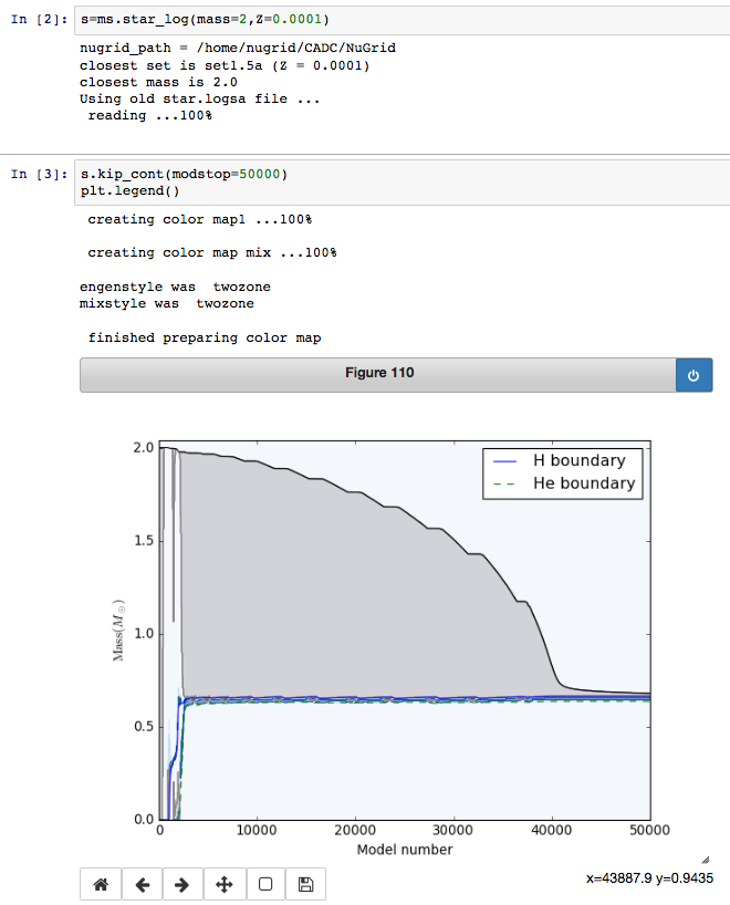
Figure 36: Example of plotting a Kippenhahn diagram in the WENDI web exploration interface that provides Jupyter notebook-based analytic access to the NuGrid stellar evolution and nucleosynthesis data.

In addition to plotting and analyzing the stellar evolution, nucleosynthesis and yield data online in the WENDI platform the raw data is also accessible online at http://nugridstars.org/data-and-software/yields/set-1. It can be read and analysed with the NuGridPy tools mentioned above. Stellar yield tables as shown in Table 12 are provided for all metallicities. Separate tables are available for contribution from stellar winds only, from winds plus pre-SN ejecta and winds plus SN ejecta. Figures of overproduction factors for all elements and many isotopes such as in Fig. 24 and in Fig. 30 are available for all metallicities. Stellar yields can be further applied and used in galactic chemical evolution models via the Stellar Yields for Galactic Modeling Applications (SYGMA) Python code (Ritter et al., 2017b) that is part of the NuGrid Python Chemical Evolution Environment NuPyCEE package (http://nugrid.github.io/NuPyCEE Côté et al., 2016b).

References

- Arnett & Meakin (2011) Arnett W. D., Meakin C., 2011, ApJ, 733, 78
- Arnould & Goriely (2003) Arnould M., Goriely S., 2003, Phys. Rep., 384, 1
- Banerjee et al. (2013) Banerjee P., Qian Y.-Z., Haxton W. C., Heger A., 2013, Physical Review Letters, 110, 141101
- Baraffe et al. (1992) Baraffe I., El Eid M. F., Prantzos N., 1992, A&A, 258, 357
- Battino et al. (2016) Battino U., et al., 2016, ApJ, 827, 30
- Belczynski et al. (2012) Belczynski K., Wiktorowicz G., Fryer C. L., Holz D. E., Kalogera V., 2012, ApJ, 757, 91
- Blöcker (1993) Blöcker T., 1993, PhD thesis, , Universität Kiel, Germany, (1993)
- Blöcker & Schönberner (1995) Blöcker T., Schönberner D., 1995, in 2nd Int. Coll. on Hydrogen-Deficient Stars.
- Busso et al. (1999) Busso M., Gallino R., Wasserburg G. J., 1999, ARA&A, 37, 239
- Busso et al. (2007) Busso M., Wasserburg G. J., Nollett K. M., Calandra A., 2007, ApJ, 671, 802
- Cameron & Fowler (1971) Cameron A. G. W., Fowler W. A., 1971, ApJ, 164, 111
- Campbell et al. (2010) Campbell S. W., Lugaro M., Karakas A. I., 2010, A&A, 522, L6
- Chen et al. (2014) Chen M. C., Herwig F., Denissenkov P. A., Paxton B., 2014, MNRAS, 440, 1274
- Chieffi & Limongi (2004) Chieffi A., Limongi M., 2004, ApJ, 608, 405
- Côté et al. (2013) Côté B., Martel H., Drissen L., 2013, ApJ, 777, 107
- Côté et al. (2016a) Côté B., West C., Heger A., Ritter C., O’Shea B. W., Herwig F., Travaglio C., Bisterzo S., 2016a, MNRAS, 463, 3755
- Côté et al. (2016b) Côté B., Ritter C., O’Shea B. W., Herwig F., Pignatari M., Jones S., Fryer C. L., 2016b, ApJ, 824, 82
- Côté et al. (2017) Côté B., O’Shea B. W., Ritter C., Herwig F., Venn K. A., 2017, ApJ, 835, 128
- Cristallo et al. (2001) Cristallo S., Straniero O., Gallino R., Herwig F., Chieffi A., Limongi M., Busso M., 2001, Nuclear Physics A, 688, 217
- Cristallo et al. (2009) Cristallo S., Piersanti L., Straniero O., Gallino R., Domínguez I., Käppeler F., 2009, Publ. Astron. Soc. Australia, 26, 139
- Cristallo et al. (2011) Cristallo S., et al., 2011, ApJS, 197, 17
- Cristallo et al. (2015) Cristallo S., Straniero O., Piersanti L., Gobrecht D., 2015, preprint, (arXiv:1507.07338)
- Cristini et al. (2016) Cristini A., Meakin C., Hirschi R., Arnett D., Georgy C., Viallet M., 2016, preprint, (arXiv:1610.05173)
- Denissenkov & Tout (2003) Denissenkov P. A., Tout C. A., 2003, MNRAS, 340, 722
- Denissenkov et al. (2009) Denissenkov P. A., Pinsonneault M., MacGregor K. B., 2009, ApJ, 696, 1823
- Denissenkov et al. (2013) Denissenkov P. A., Herwig F., Truran J. W., Paxton B., 2013, ApJ, 772, 37
- Denissenkov et al. (2017) Denissenkov P. A., Herwig F., Battino U., Ritter C., Pignatari M., Jones S., Paxton B., 2017, ApJ, 834, L10
- Doherty et al. (2010) Doherty C. L., Siess L., Lattanzio J. C., Gil-Pons P., 2010, MNRAS, 401, 1453
- Doherty et al. (2014) Doherty C. L., Gil-Pons P., Lau H. H. B., Lattanzio J. C., Siess L., Campbell S. W., 2014, MNRAS, 441, 582
- Eggenberger et al. (2008) Eggenberger P., Meynet G., Maeder A., Hirschi R., Charbonnel C., Talon S., Ekström S., 2008, Ap&SS, 316, 43
- Ekström et al. (2008) Ekström S., Meynet G., Chiappini C., Hirschi R., Maeder A., 2008, A&A, 489, 685
- El Eid et al. (2004) El Eid M. F., Meyer B. S., The L.-S., 2004, ApJ, 611, 452
- Farmer et al. (2015) Farmer R., Fields C. E., Timmes F. X., 2015, ApJ, 807, 184
- Few et al. (2012) Few C. G., Courty S., Gibson B. K., Kawata D., Calura F., Teyssier R., 2012, MNRAS, 424, L11
- Fishlock et al. (2014) Fishlock C. K., Karakas A. I., Lugaro M., Yong D., 2014, ApJ, 797, 44
- Freytag et al. (1996) Freytag B., Ludwig H.-G., Steffen M., 1996, A&A, 313, 497
- Frischknecht et al. (2016) Frischknecht U., et al., 2016, MNRAS, 456, 1803
- Frost et al. (1998) Frost C. A., Cannon R. C., Lattanzio J. C., Wood P. R., Forestini M., 1998, A&A, 332, L17
- Fryer (1999) Fryer C. L., 1999, ApJ, 522, 413
- Fryer et al. (2012) Fryer C. L., Belczynski K., Wiktorowicz G., Dominik M., Kalogera V., Holz D. E., 2012, ApJ, 749, 91
- Fujimoto et al. (2000) Fujimoto M. Y., Ikeda Y., Iben I. J., 2000, ApJ Lett., 529, L25
- Gallino et al. (1998) Gallino R., Arlandini C., Busso M., Lugaro M., Travaglio C., Straniero O., Chieffi A., Limongi M., 1998, ApJ, 497, 388
- García-Berro et al. (1997) García-Berro E., Ritossa C., Iben Jr. I., 1997, ApJ, 485, 765
- García-Hernández et al. (2013) García-Hernández D. A., Zamora O., Yagüe A., Uttenthaler S., Karakas A. I., Lugaro M., Ventura P., Lambert D. L., 2013, A&A, 555, L3
- Gibson (2002) Gibson B. K., 2002, in Nomoto K., Truran J. W., eds, IAU Symposium Vol. 187, Cosmic Chemical Evolution. pp 159–163
- Gil-Pons & Doherty (2010) Gil-Pons P., Doherty C. L., 2010, Mem. Soc. Astron. Italiana, 81, 974
- Gil-Pons et al. (2013) Gil-Pons P., Doherty C. L., Lau H., Campbell S. W., Suda T., Guilani S., Gutiérrez J., Lattanzio J. C., 2013, A&A, 557, A106
- Glebbeek et al. (2009) Glebbeek E., Gaburov E., de Mink S. E., Pols O. R., Portegies Zwart S. F., 2009, A&A, 497, 255
- Goriely & Siess (2004) Goriely S., Siess L., 2004, A&A, 421, L25
- Grevesse & Noels (1993) Grevesse N., Noels A., 1993, in N. Prantzos, E. Vangioni-Flam, & M. Casse ed., Origin and Evolution of the Elements. pp 15–25
- Gutierrez et al. (1996) Gutierrez J., Garcia-Berro E., Iben Jr. I., Isern J., Labay J., Canal R., 1996, ApJ, 459, 701
- Heger & Woosley (2010) Heger A., Woosley S. E., 2010, ApJ, 724, 341
- Herant et al. (1994) Herant M., Benz W., Hix W. R., Fryer C. L., Colgate S. A., 1994, ApJS
- Herwig (2000) Herwig F., 2000, A&A, 360, 952
- Herwig (2001a) Herwig F., 2001a, APSS, 275, 15
- Herwig (2001b) Herwig F., 2001b, ApJ Lett., 554, L71
- Herwig (2004a) Herwig F., 2004a, ApJS, 155, 651
- Herwig (2004b) Herwig F., 2004b, ApJ, 605, 425
- Herwig (2005) Herwig F., 2005, ARA&A, 43, 435
- Herwig & Langer (2001) Herwig F., Langer N., 2001, Nuclear Physics A, 688, 221
- Herwig et al. (1997) Herwig F., Blöcker T., Schönberner D., El Eid M. F., 1997, A&A, 324, L81
- Herwig et al. (1998) Herwig F., Schönberner D., Blöcker T., 1998, A&A, 340, L43
- Herwig et al. (1999) Herwig F., Blöcker T., Langer N., Driebe T., 1999, A&A, 349, L5
- Herwig et al. (2003) Herwig F., Langer N., Lugaro M., 2003, ApJ, 593, 1056
- Herwig et al. (2007) Herwig F., Freytag B., Fuchs T., Hansen J. P., Hueckstaedt R. M., Porter D. H., Timmes F. X., Woodward P. R., 2007, in Kerschbaum F., Charbonnel C., Wing R. F., eds, Astronomical Society of the Pacific Conference Series Vol. 378, Why Galaxies Care About AGB Stars: Their Importance as Actors and Probes. p. 43 (arXiv:0709.0197)
- Herwig et al. (2011) Herwig F., Pignatari M., Woodward P. R., Porter D. H., Rockefeller G., Fryer C. L., Bennett M., Hirschi R., 2011, ApJ, 727, 89
- Herwig et al. (2014) Herwig F., Woodward P. R., Lin P.-H., Knox M., Fryer C., 2014, ApJ, 792, L3
- Herwig et al. (2018) Herwig F., et al., 2018, ASTROPHYS J SUPPL S, 236, 2
- Hirschi (2007) Hirschi R., 2007, A&A, 461, 571
- Hirschi et al. (2004) Hirschi R., Meynet G., Maeder A., 2004, A&A, 425, 649
- Hirschi et al. (2005) Hirschi R., Meynet G., Maeder A., 2005, A&A, 433, 1013
- Iben & MacDonald (1995) Iben Jr. I., MacDonald J., 1995, in Koester D., Werner K., eds, White Dwarfs. No. 443 in LNP. Springer, Heidelberg, p. 48
- Iben & Renzini (1982) Iben Jr. I., Renzini A., 1982, ApJ, 259, L79
- Iben et al. (1983) Iben Jr. I., Kaler J. B., Truran J. W., Renzini A., 1983, ApJ, 264, 605
- Iwamoto et al. (2004) Iwamoto N., Kajino T., Mathews G. J., Fujimoto M. Y., Aoki W., 2004, ApJ, 602, 378
- Janka et al. (2007) Janka H.-T., Langanke K., Marek A., Martínez-Pinedo G., Müller B., 2007, Phys. Rep., 442, 38
- Jones et al. (2013) Jones S., et al., 2013, ApJ, 772, 150
- Jones et al. (2014) Jones S., Hirschi R., Nomoto K., 2014, ApJ, 797, 83
- Jones et al. (2015) Jones S., Hirschi R., Pignatari M., Heger A., Georgy C., Nishimura N., Fryer C., Herwig F., 2015, MNRAS, 447, 3115
- Jones et al. (2016) Jones S., Ritter C., Herwig F., Fryer C., Pignatari M., Bertolli M. G., Paxton B., 2016, MNRAS, 455, 3848
- Jones et al. (2017) Jones S., Andrassy R., Sandalski S., Davis A., Woodward P., Herwig F., 2017, MNRAS, 465, 2991
- Käppeler et al. (1989) Käppeler F., Beer H., Wisshak K., 1989, Rep. Prog. Phys., 52, 945
- Käppeler et al. (2011) Käppeler F., Gallino R., Bisterzo S., Aoki W., 2011, Reviews of Modern Physics, 83, 157
- Karakas (2003) Karakas A., 2003, Ph.D. Thesis,
- Karakas (2010) Karakas A. I., 2010, VizieR Online Data Catalog, 740, 31413
- Karakas & Lugaro (2016) Karakas A. I., Lugaro M., 2016, ApJ, 825, 26
- Karakas et al. (2012) Karakas A. I., García-Hernández D. A., Lugaro M., 2012, ApJ, 751, 8
- Kobayashi et al. (2006) Kobayashi C., Umeda H., Nomoto K., Tominaga N., Ohkubo T., 2006, ApJ, 653, 1145
- Lattanzio & Boothroyd (1997) Lattanzio J. C., Boothroyd A. I., 1997, in Bernatowitz T., Zinner E., eds, Astrophysical Implications of the Laboratory Study of Presolar Materials. AIP Conf. Ser., p. 85
- Lattanzio et al. (1996) Lattanzio J., Frost C., Cannon R., Wood P. R., 1996, Mem. Soc. Astron. Italiana, 67, 729
- Lattanzio et al. (1997) Lattanzio J. C., Frost C. A., Cannon R. C., Wood P. R., 1997, Nuclear Physics A, 621, 435
- Limongi & Chieffi (2006) Limongi M., Chieffi A., 2006, ApJ, 647, 483
- Lodders (2003) Lodders K., 2003, ApJ
- Lugaro et al. (2003) Lugaro M., Herwig F., Lattanzio J. C., Gallino R., Straniero O., 2003, ApJ, 586, 1305
- Lugaro et al. (2012) Lugaro M., Karakas A. I., Stancliffe R. J., Rijs C., 2012, ApJ, 747, 2
- Maeder & Meynet (2001) Maeder A., Meynet G., 2001, A&A, 373, 555
- Magkotsios et al. (2010) Magkotsios G., Timmes F., Hungerford A., Fryer C., Young P., Wiescher M., 2010, in APS Division of Nuclear Physics Meeting Abstracts. p. H5
- Marigo (2001) Marigo P., 2001, A&A, 370, 194
- Mattsson et al. (2010) Mattsson L., Wahlin R., Höfner S., 2010, A&A, 509, A14
- Meakin & Arnett (2006) Meakin C. A., Arnett D., 2006, ApJ Lett., 637, L53
- Meakin & Arnett (2007) Meakin C. A., Arnett D., 2007, ApJ, 665, 690
- Meyer et al. (2000) Meyer B. S., Clayton D. D., The L.-S., 2000, ApJ, 540, L49
- Meynet & Maeder (2002) Meynet G., Maeder A., 2002, A&A, 390, 561
- Mollá et al. (2015) Mollá M., Cavichia O., Gavilán M., Gibson B. K., 2015, MNRAS, 451, 3693
- Müller (2016) Müller B., 2016, Publ. Astron. Soc. Australia, 33, e048
- Nomoto et al. (2006) Nomoto K., Tominaga N., Umeda H., Kobayashi C., Maeda K., 2006, Nuclear Physics A, 777, 424
- Nomoto et al. (2013) Nomoto K., Kobayashi C., Tominaga N., 2013, ARA&A, 51, 457
- Nugis & Lamers (2000) Nugis T., Lamers H. J. G. L. M., 2000, A&A, 360, 227
- Paxton et al. (2011) Paxton B., Bildsten L., Dotter A., Herwig F., Lesaffre P., Timmes F., 2011, ApJS, 192, 3
- Peters (1968) Peters J. G., 1968, ApJ, 154, 225
- Peters & Hirschi (2013) Peters G. J., Hirschi R., 2013, The Evolution of High-Mass Stars. p. 447, doi:10.1007/978-94-007-5615-1_9
- Pignatari & Gallino (2007) Pignatari M., Gallino R., 2007, Mem. Soc. Astron. Italiana, 78, 543
- Pignatari et al. (2010) Pignatari M., Gallino R., Heil M., Wiescher M., Käppeler F., Herwig F., Bisterzo S., 2010, ApJ, 710, 1557
- Pignatari et al. (2013a) Pignatari M., et al., 2013a, ApJ, 767, L22
- Pignatari et al. (2013b) Pignatari M., et al., 2013b, ApJ, 771, L7
- Pignatari et al. (2015) Pignatari M., et al., 2015, preprint, (arXiv:1506.09056)
- Pignatari et al. (2016a) Pignatari M., Göbel K., Reifarth R., Travaglio C., 2016a, International Journal of Modern Physics E, 25, 1630003
- Pignatari et al. (2016b) Pignatari M., et al., 2016b, The Astrophysical Journal Supplement Series, 225, 24
- Pignatari et al. (2017) Pignatari M., Hoppe P., Trappitsch T., Fryer C., Timmes F., Herwig F., Hirschi R., 2017, Geochim. Cosmochim. Acta, 5, 6
- Portinari et al. (1998) Portinari L., Chiosi C., Bressan A., 1998, A&A, 334, 505
- Prantzos (2000) Prantzos N., 2000, New Astron. Rev., 44, 303
- Prantzos (2012) Prantzos N., 2012, A&A, 542, A67
- Prantzos et al. (1990) Prantzos N., Hashimoto M., Nomoto K., 1990, A&A, 234, 211
- Raiteri et al. (1992) Raiteri C. M., Gallino R., Busso M., 1992, ApJ, 387, 263
- Rauscher et al. (2002) Rauscher T., Heger A., Hoffman R. D., Woosley S. E., 2002, ApJ, 576, 323
- Rauscher et al. (2013) Rauscher T., Dauphas N., Dillmann I., Fröhlich C., Fülöp Z., Gyürky G., 2013, Reports on Progress in Physics, 76, 066201
- Rauscher et al. (2016) Rauscher T., Nishimura N., Hirschi R., Cescutti G., Murphy A. S. J., Heger A., 2016, MNRAS, 463, 4153
- Rayet et al. (1995) Rayet M., Arnould M., Hashimoto M., Prantzos N., Nomoto K., 1995, A&A, 298, 517
- Reddy et al. (2006) Reddy B. E., Lambert D. L., Allende Prieto C., 2006, VizieR Online Data Catalog, 736, 71329
- Reimers (1975) Reimers D., 1975, Mem. Soc. Sci. Liege, 8, 369
- Ritossa et al. (1999) Ritossa C., García-Berro E., Iben I. J., 1999, ApJ, 515, 381
- Ritter et al. (2017a) Ritter C., Andrassy R., Côté B., Herwig F., Woodward P. R., Pignatari M., Jones S., 2017a, MNRAS,
- Ritter et al. (2017b) Ritter C., Côté B., Herwig F., Navarro J. F., Fryer C., 2017b, ApJS
- Romano et al. (2010) Romano D., Karakas A. I., Tosi M., Matteucci F., 2010, A&A, 522, A32
- Rosenfield et al. (2014) Rosenfield P., et al., 2014, ApJ, 790, 22
- Sackmann & Boothroyd (1992) Sackmann I.-J., Boothroyd A. I., 1992, ApJ, 392, L71
- Sbordone et al. (2010) Sbordone L., et al., 2010, A&A, 522, A26
- Scalo et al. (1975) Scalo J. M., Despain K. H., Ulrich R. K., 1975, ApJ, 196, 805
- Scannapieco et al. (2005) Scannapieco C., Tissera P. B., White S. D. M., Springel V., 2005, MNRAS, 364, 552
- Schaye et al. (2015) Schaye J., et al., 2015, MNRAS, 446, 521
- Siess (2007) Siess L., 2007, A&A, 476, 893
- Siess (2010) Siess L., 2010, A&A, 512, A10
- Straniero et al. (1995) Straniero O., Gallino R., Busso M., Chieffi A., Raiteri C. M., Salaris M., Limongi M., 1995, ApJ, 440, L85
- Straniero et al. (2014) Straniero O., Cristallo S., Piersanti L., 2014, ApJ, 785, 77
- Sukhbold & Woosley (2014) Sukhbold T., Woosley S. E., 2014, ApJ, 783, 10
- Sukhbold et al. (2016) Sukhbold T., Ertl T., Woosley S. E., Brown J. M., Janka H.-T., 2016, ApJ, 821, 38
- The et al. (2007) The L., El Eid M. F., Meyer B. S., 2007, ApJ, 655, 1058
- Thielemann et al. (1979) Thielemann F.-K., Arnould M., Hillebrandt W., 1979, A&A, 74, 175
- Trippella et al. (2016) Trippella O., Busso M., Palmerini S., Maiorca E., Nucci M. C., 2016, ApJ, 818, 125
- Ugliano et al. (2012) Ugliano M., Janka H.-T., Marek A., Arcones A., 2012, ApJ, 757, 69
- Vassiliadis & Wood (1993) Vassiliadis E., Wood P., 1993, ApJ, 413, 641
- Ventura & D’Antona (2011) Ventura P., D’Antona F., 2011, MNRAS, 410, 2760
- Ventura et al. (2013) Ventura P., Di Criscienzo M., Carini R., D’Antona F., 2013, MNRAS, 431, 3642
- Ventura et al. (2015) Ventura P., Karakas A. I., Dell’Agli F., Boyer M. L., García-Hernández D. A., Di Criscienzo M., Schneider R., 2015, MNRAS, 450, 3181
- Vink et al. (2001) Vink J. S., de Koter A., Lamers H. J. G. L. M., 2001, A&A, 369, 574
- Weiss & Ferguson (2009) Weiss A., Ferguson J. W., 2009, A&A, 508, 1343
- Willson (2000) Willson L. A., 2000, ARA&A, 38, 573
- Woosley & Hoffman (1992) Woosley S. E., Hoffman R. D., 1992, ApJ, 395, 202
- Woosley & Howard (1978) Woosley S. E., Howard W. M., 1978, ApJS, 36, 285
- Woosley & Weaver (1995) Woosley S. E., Weaver T. A., 1995, APJS, 101, 181+
- Woosley et al. (1973) Woosley S. E., Arnett W. D., Clayton D. D., 1973, ApJS, 26, 231
- Woosley et al. (2002) Woosley S. E., Heger A., Weaver T. A., 2002, Rev. Mod. Phys., 74, 1015
- Young et al. (2009) Young P. A., Ellinger C. I., Arnett D., Fryer C. L., Rockefeller G., 2009, ApJ, 699, 938
- Zinner (2014) Zinner E., 2014, Treatise on Geochemistry, 2nd edition, 1, 181
- de Jager et al. (1988) de Jager C., Nieuwenhuijzen H., van der Hucht K. A., 1988, A&AS, 72, 259
- van Loon (2000) van Loon J. T., 2000, A&A, 354, 125
- van Loon et al. (2005) van Loon J. T., Cioni M.-R. L., Zijlstra A. A., Loup C., 2005, A&A, 438, 273