The coalescing colony model: mean-field, scaling, and geometry

Abstract

We analyze the coalescing model where a ‘primary’ colony grows and randomly emits secondary colonies that spread and eventually coalesce with it. This model describes population proliferation in theoretical ecology, tumor growth and is also of great interest for modeling the development of cities. Assuming the primary colony to be always spherical of radius $r(t)$ and the emission rate proportional to $r(t)^{\theta}$ where $\theta>0$, we derive the mean-field equations governing the dynamics of the primary colony, calculate the scaling exponents versus $\theta$ and compare our results with numerical simulations. We then critically test the validity of the circular approximation and show that it is sound for a constant emission rate ($\theta=0$). However, when the emission rate is proportional to the perimeter, the circular approximation breaks down and the roughness of the primary colony can not be discarded, thus modifying the scaling exponents.

Dispersal models have been used extensively to investigate the proliferation of animal colonies in theoretical ecology Shigesada:1997 ; Clark:2001 and as a simplified model for the growth of cancerous tumors Iwata:2000 ; Haustein:2012 . Such models are also good candidates for describing the growth of the built-area of cities Barthelemy:2016 for which we now have empirical data over long periods of time Angel:2005 . The main feature of dispersal models is the concomitant existence of two growth mechanisms. The first process is the growth of the main – so-called primary – colony, which occurs via a reaction-diffusion process (as described by a FKK-like equation Fisher:1937 ; Shigesada:2002 ) and leads to a constant growth with velocity $c$, depending on the details of the system. The second ingredient is random dispersal from the primary colony, which represents the emergence of secondary settlements in the framework of animal ecology, the development of metastatic tumors, or, in the urban sprawl case, the creation of small towns in the periphery of large cities. In the real world, dispersion follows privileged directions under the effect of external forces such as blood vessels, winds and rivers, or transportation networks for cities but in a first approach, these anisotropic effects will be neglected. We will assume that secondary colonies also grow at the velocity $c$ and will eventually coalesce with the primary colony, leading to a larger primary colony whose time-dependent size will depend on the emission rate.

A classical way to study dispersal is through the dispersal kernel representing the probability distribution of dispersal distances and various forms for these kernels have been discussed Lewis:2016 . A different approach has been introduced by Kawasaki and Shigesada in Shigesada:1997 ; Shigesada:2002 who proposed the use of simple models to tackle this challenging problem. We shall follow this point of view and study the coalescing colony model where a primary colony grows at radial velocity $c$ and emits a secondary colony at a rate $\lambda$ and at a distance $\ell$ from its border (long-range dispersal). The variable $\ell$ can be drawn from a probability distribution $P(\ell)$ but we consider here that the secondary colonies are emitted at a constant distance $\ell_{0}$ from the boundary of the primary colony (i.e. $P(\ell)=\delta(\ell-\ell_{0})$). Besides, we assume that each secondary colony also grows with the same radial speed $c$ and does not emit tertiary colonies. The dependence of the emission rate on the colony size is taken into account by the functional form

$$\lambda(r)=\lambda_{0}r^{\theta}~{},$$ (1)

$r$ being the radius of the primary colony and $\theta\geq 0$. When $\theta=0$ the growth rate is independent from the primary colony size, for $\theta=1$ it is proportional to its perimeter and for $\theta=2$ to its area.

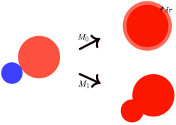
Coalescence happens when a secondary colony of radius $r_{2}$ intersects with the primary one, of radius $r$, and becomes part of the latter. We shall consider two variants of the process. In the first version of the model, denoted by the $M_{0}$ model, we assume that the primary colony remains circular after coalescence (see Fig. 1), and has a new radius $r^{\prime}$ given by

$${r^{\prime}}^{2}=r^{2}+r_{2}^{2}~{}.$$ (2)

This interesting model was discussed in Shigesada:2002 but a full quantitative understanding of the radius $r(t)$ is still lacking. Here, we present a microscopic derivation of the dynamics of the $M_{0}$ model, in the mean-field approximation, and study its solutions as a function of the parameter $\theta$. In particular, we derive a simplified equation that preserves the physics of the system and allows to extract the scaling behavior for the main quantities of interest. Our predictions are then tested with numerical simulations.

In the second part of this work, we discuss the importance of the circular approximation and its impact on the scaling behaviors. We introduce a modified version of the process, referred to as the $M_{1}$ model, in which after coalescence the secondary colony merges into the primary colony and the shape of the primary colony does not remain circular. This important difference between models $M_{0}$ and $M_{1}$ is illustrated in the Fig. 1.

Figure 1: Example of coalescence in models $M_{0}$ and $M_{1}$. In $M_{0}$, the primary colony (in red) remains circular and the area of the secondary colony is evenly distributed on the rim; in $M_{1}$, the shapes are simply ‘concatenated’.

We now derive the main equations for the model $M_{0}$. We recall that $\lambda(t_{i})dt_{i}$ represents the probability to emit a colony in the interval $[t_{i},t_{i}+dt_{i}]$ and we denote by ${t_{i}}^{\prime}$ the time of coalescence of a colony emitted at time $t_{i}$. The condition of coalescence is given by

$$r({t_{i}}^{\prime})+c{t_{i}}^{\prime}=\ell_{0}+r(t_{i})+ct_{i}~{},$$ (3)

which defines – formally – the function $f$ such that

$${t_{i}}^{\prime}=f(t_{i})~{}.$$ (4)

The mean-field approach that we propose here consists in neglecting the fluctuations of this function $f(t)$ and to consider that it is the same for all secondary colonies. The evolution of the area of the primary colony is thus given by

$$\frac{dA}{dt}=2\pi rc+\int d{t_{i}}\lambda(t_{i}){\delta}(t-f(t_{i}))\pi c^{2}(t-t_{i})^{2}~{},$$ (5)

where the first term of the rhs is due to short-range dispersion and the second term represents the coalescence with secondary colonies. This leads to

$$\frac{dA}{dt}=2\pi rc+\lambda(f^{-1}(t))\mid\left[f^{-1}(t)\right]^{\prime}\pi c^{2}(t-f^{-1}(t))^{2}\mid~{}.$$ (6)

We call $x(t)$ the radius of the colony absorbed at time $t$, given by $x(t)=c(t-f^{-1}(t))$. Injecting this quantity in Eqs. (3) and (6), we obtain the Kawasaki-Shigesada system of equations Shigesada:2002

$$\frac{dr}{dt} =c+\frac{\lambda_{0}{\left[r\left(t-\frac{x(t)}{c}\right)\right]}^{\theta}}{2\pi r(t)}\left(1-\frac{\dot{x}(t)}{c}\right)\pi x(t)^{2}~{},$$ (7)

$$\ell_{0} =r(t)-r\left(t-\frac{x(t)}{c}\right)+x(t)~{}.$$ (8)

In the long time regime, $t\gg x(t)/c$, the system of Eq. (7) and Eq. (8) takes the simplified form

$$\frac{dr}{dt} =c+\frac{\lambda_{0}r^{\theta-1}}{2}x(t)^{2}~{},$$ (9)

$$x(t) =\frac{\ell_{0}}{1+\frac{\dot{r}}{c}}~{}.$$ (10)

These effective equations allow us to investigate the behavior of the model without altering the physics of the problem as will be shown by comparing the solutions to numerical simulations.

We first solve the effective system for $\theta=0$ (ie. $\lambda=\lambda_{0}$). Defining $x^{*}$ as the average radius of a secondary colony just before its coalescence and assuming that it is constant in time we obtain

$$\frac{dr}{dt}=c+\frac{\lambda_{0}}{2r}{x^{*}}^{2}~{},$$ (11)

whose solution is

$$r(t)\sim a+ct+\frac{\lambda_{0}{x^{*}}^{2}}{2c}\log{\left(\frac{2cr}{\lambda_{0}{x^{*}}^{2}}+1\right)}~{}.$$ (12)

When $t\to\infty$, the dominant contribution is

$$r(t)\sim a+ct+\frac{\mathscr{C}}{c}\log{\left(\frac{c^{2}t}{\mathscr{C}}+1\right)}~{},$$ (13)

with $x^{*}\simeq\ell_{0}/2$ and $\mathscr{C}=\frac{\lambda l_{0}^{2}}{8}$.

We perform numerical simulations with a constant $\lambda_{0}=0.5$ and $c=1$, for different values of the emission distance $\ell_{0}$. It is useful to introduce $\eta=\frac{2c}{l_{0}\lambda_{0}}$, which represents the ratio between the emission time $\tau_{e}=1/\lambda_{0}$ and the coalescence time $\tau_{c}=\ell_{0}/(2c)$. In Fig. 2 Top-Left, we plot the radius of the primary colony $r(t)$ versus $t$. We then perform on these data a two parameters fit with a function of the form

$$g(t)=a+\frac{\mathscr{C}_{simul}}{c}\log{\left(\frac{c^{2}t}{\mathscr{C}_{simul}}+1\right)}~{},$$ (14)

where the fitting parameters are $a$ and $\mathscr{C}_{simul}$.

Figure 2: (Top) Case $\theta=0$: (Top-Left) Plot of $r(t)$ versus $t$ for different values of the parameter $\eta$, averaged over $10$ simulations. (Top-Right) Plot of $\mathscr{C}_{simul}$ versus $\eta$ extracted from the empirical fit. The theoretical prediction is shown in red. (Bottom) Case $\theta=1$: (Bottom-Left) $r(t)$ versus $t$ for different values of the parameter $\eta$, obtained averaging over $100$ simulations. (Bottom-Right) $c^{\prime}-c$ versus $\eta$ as obtained from the empirical fit. In red, the theoretical prediction (Eq. (18)).

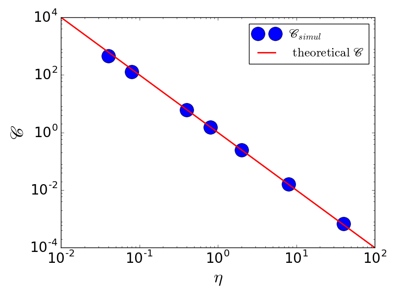
In Fig. 2 Top-Right we test the results of the fit, comparing the estimated value $\mathscr{C}_{simul}$ obtained, with its theoretical value $\mathscr{C}=\frac{\lambda l_{0}^{2}}{8}=\frac{c^{2}}{2\lambda_{0}\eta^{2}}$. We observe an excellent agreement, showing the validity of our theoretical calculations.

For $\theta>1$, we further simplify the system Eqs. (26) and (27) by assuming $\dot{r}\gg c$ and obtain the single effective equation

$$Ar(t)^{\theta-1}\simeq\dot{r(t)}^{2}\left(\dot{r(t)}-c\right)$$ (15)

with $A=\frac{\lambda_{0}}{2}c^{2}\ell_{0}^{2}$. This nonlinear differential equation captures the physics of the coalescence and allows us to extract the large-time behavior of the main quantities of interest in this problem. In particular, assuming scaling laws at large times of the form $r(t)\sim at^{\beta}$ and $x(t)\sim dt^{-\alpha}$, Eq. 15 yields

$$\beta=\frac{3}{4-\theta}~{},\qquad\qquad\alpha=\beta-1~{}.$$ (16)

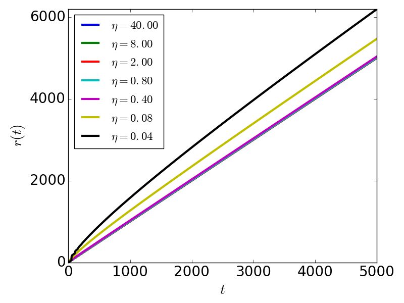
Note that for $\theta\rightarrow 4$, we have $\beta\rightarrow\infty$, the radius grows faster than a power law and explodes exponentially. For $\theta=1$, we obtain $\alpha=0,\beta=1$ which means that we have $x(t)=x^{*}$ independent of $t$ and a linear behavior of $r(t)$. From Eq. (7) we deduce that the radial velocity $c^{\prime}$ is given by

$$c^{\prime}=c+\frac{\lambda_{0}}{2}{x^{*}}^{2}$$ (17)

and the value of $x^{*}$ can be obtained by solving Eq. (8) that can be written as

$$\frac{\lambda_{0}}{2c}{x^{*}}^{3}+2{x^{*}}-\ell_{0}=0~{}.$$ (18)

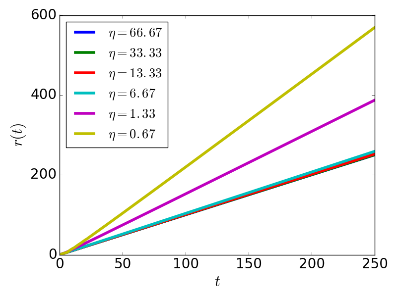
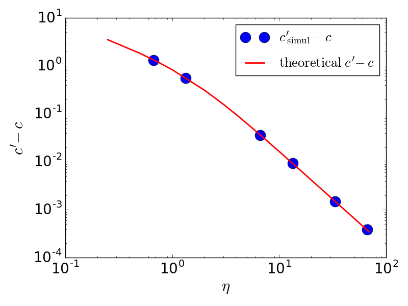
This result, for the specific case of $\theta=1$, was first obtained by Shigesada and Kawasaki Shigesada:1997 . We test this result numerically (with $\lambda_{0}=0.3$, $c=1$, and for different values of the emission distance $\ell_{0}$) and in Fig. 2 Bottom-Left we plot the radius of the primary colony $r(t)$ versus $t$. A linear fit allows us to obtain an estimate for the radial velocity $c^{\prime}$ that we compare in Fig. 2 Bottom-Right with the theoretical prediction of Eq. (18). Here also, an excellent agreement is observed.

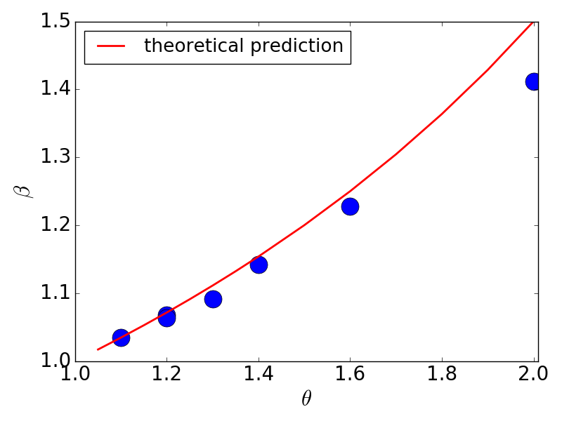
For $\theta>1$, the theoretical analysis predicts that the leading order characterized by a scaling behavior given by Eqs. (16) can be observed in a range of time $t_{min}\ll t\ll t_{max}$ which depend on $\theta$ and on the parameter $\eta^{2}\lambda/2$ (see the supplementary material for details on this point). We performed numerical simulations for $\theta=[1.1,1.2,1.3,1.4,1.6,2.0]$, with the parameter $c=1$ and $\lambda=0.001$ (and additional simulations with the parameter $\lambda=0.005$ for $\theta=1.2$). In Fig. 3, we plot the values of the exponents $\beta$ obtained by power law fits and we compare it with the theoretical prediction (Eq. (16)) in red. We observe a good agreement with some deviations for higher values of $\theta$ which is probably due the small range $[t_{min},t_{max}]$ in this case.

Figure 3: Plot of the exponent $\beta$ as a function of $\theta$, obtained from a power law fit on $r(t)$ versus $t$ for the values of $\eta^{2}\lambda/2$ maximizing the range $[t_{min},t_{max}]$ in our simulation domain.

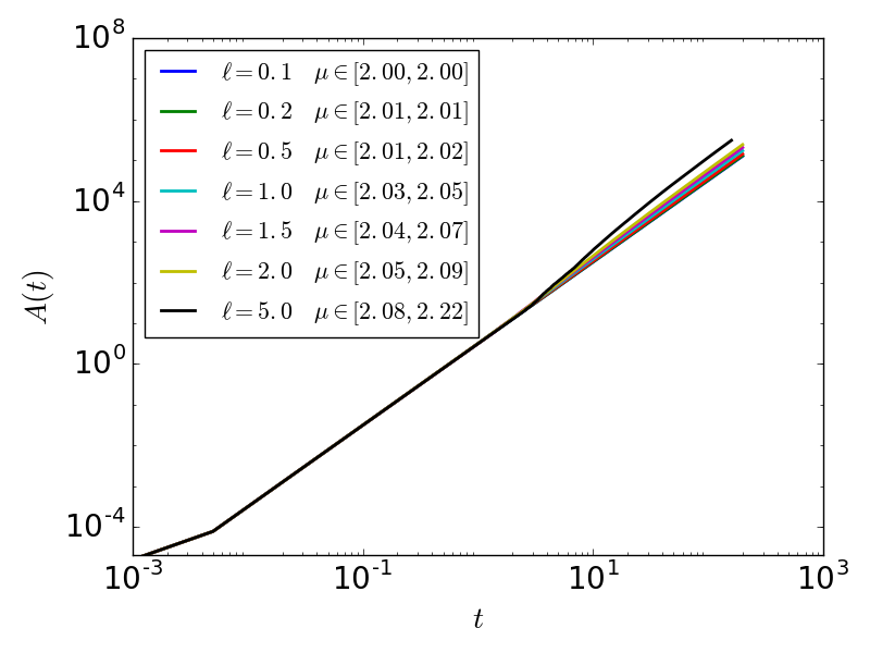
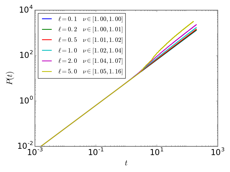
The Shigesada-Kawasaki coalescing model is based on the circular approximation. The validity of this hypothesis will be investigated by simulating the $M_{1}$ model where we respect the geometry of the coalescence process. We first consider a constant emission rate $\lambda(r)=\lambda_{0}$ and assume that the area $A$ and the perimeter $P$ obey to a power law scaling of the form

$$A(t)\sim t^{\mu}\qquad P(t)\sim t^{\nu}~{}.$$ (19)

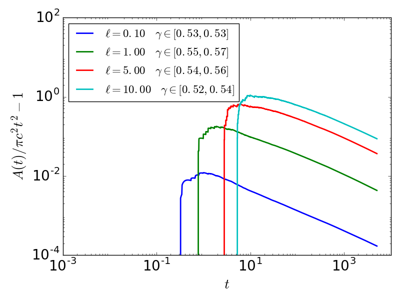
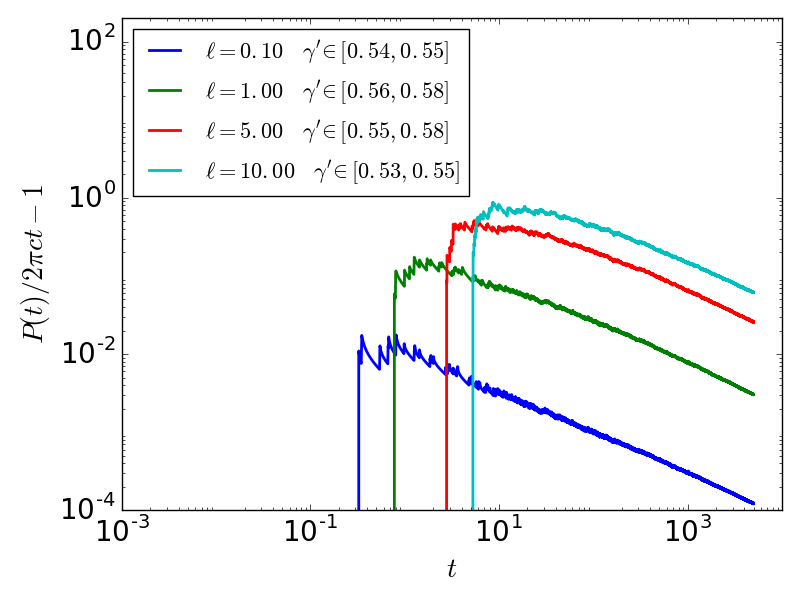
Performing a power-law fit on the empirical results, we obtain $\mu\approx 2$ and $\nu\approx 1$ (see Supplementary Material for details and plots). These results can be compared with those obtained in the model $M_{0}$. In Fig. 4, we plot $A(t)/(\pi c^{2}t^{2})-1$ and $P(t)/(2\pi ct)-1$ versus $t$: these quantities both go to zero for large values of $t$, suggesting that at large times, the dominant behavior of the $M_{0}$ and the $M_{1}$ models are the same with $A(t)\sim\pi c^{2}t^{2}$ and $P(t)\sim 2\pi ct$. Hence, for $\theta=0$ and large value of $t$, the circular approximation appears to be valid.

Figure 4: (Left) $A(t)/(\pi c^{2}t^{2})-1$ versus time $t$. (Right) $P(t)/(2\pi ct)-1$ versus $t$. These results are obtained for different values of $\ell$ and are averaged over $100$ numerical simulations. For each value of $\ell$, we report in the inset the values of the exponents $\gamma$ and $\gamma^{\prime}$ obtained by fitting these plots.

If we assume that the sub-dominant corrections are described by the scaling forms

$$\frac{A(t)}{\pi c^{2}t^{2}}-1\sim t^{-\gamma}\qquad\quad\frac{P(t)}{2\pi ct}-1\sim t^{-\gamma^{\prime}}$$ (20)

the numerical results suggest that $\gamma\sim 0.5$ and $\gamma^{\prime}\sim 0.5$ showing that the corrections to the dominant term are decaying as a power law in model $M_{1}$, in contrast with the logarithmic correction observed in the $M_{0}$ model (see Supplementary Material).

We now focus on the simulation results obtained for the $M_{1}$ model characterized by an emission rate $\lambda$ given by

$$\lambda(t)=\lambda_{0}P(t)~{},$$ (21)

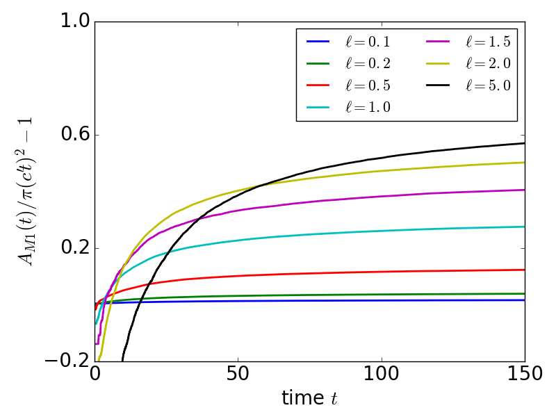
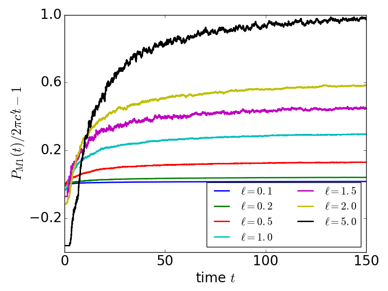
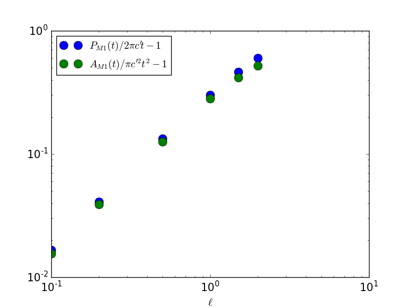
where $P(t)$ is the total perimeter of the primary colony at time $t$, which corresponds to the case $\theta=1$ in the model $M_{0}$. The simulations results for the area $A(t)$ and the perimeter $P(t)$ of the primary colony (see Supp. Mat.) suggest that we still have $\mu\approx 2$ and $\nu\approx 1$ as in the $M_{0}$ model. We can go further and investigate the prefactor. We recall that for the $M_{0}$ model with $\theta=1$, the radius of the primary colony increases with an effective radial velocity $c^{\prime}>c$. In Fig. 5 we plot the quantities $A(t)/\pi c^{\prime 2}t^{2}-1$ and $P(t)/2\pi c^{\prime}t-1$; if the prefactor is the same of the $M_{0}$ model we should find (as we did for $\theta=0$) that these quantities tend to zero for large values of $t$. In Fig. 5-(a)-(b), we see that these two quantities tend to a constant that depends on $\ell$. We can therefore write

$$A(t)=\pi c^{\prime 2}(1+f_{1}(\ell))t^{2}\qquad P(t)=2\pi c^{\prime}(1+f_{2}(\ell))t~{}.$$ (22)

and we observe numerically that $f_{1}\equiv f_{2}$ (see Fig. 5-(c)), demonstrating that the circular approximation is not appropriate for $\theta=1$.

(a)

(b)

(c)

Figure 5: (a) $A(t)/(\pi c^{2}t^{2})-1$ versus $t$ for different values of $\ell$. (b) $P(t)/(2\pi ct)-1$ versus $t$ for different values of $\ell$. (c) Plot of $f_{1}(\ell)$ and $f_{2}(\ell)$ versus $\ell$ for $t=200$. These results are obtained by averaging over $100$ simulations.

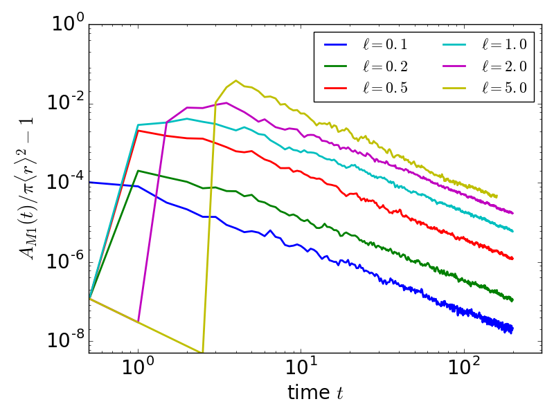
In order to shed some light on this behavior, we plot the quantities $\frac{A(t)}{\pi{\langle r\rangle}^{2}}-1$ and $\frac{P(t)}{2\pi{\langle r\rangle}}-1$ where $\langle r\rangle$ is the average radius of the primary colony.

Figure 6: (Left) $\frac{\pi{\langle r\rangle}^{2}}{A(t)}-1$ versus $t$ for different values of $\ell$. (Right) $\frac{P(t)}{2\pi{\langle r\rangle}}-1$ for different values of $\ell$. The results are obtained averaging over $100$ simulations.

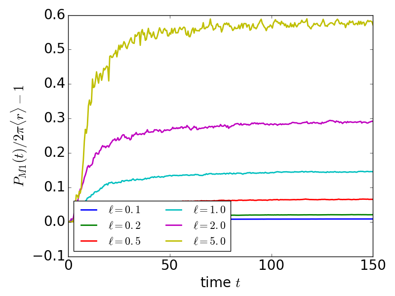The results shown in Fig. 6 suggest that the perimeter cannot be described by a circle, signaling a breakdown of the circular approximation (even if from the point of view of the area the system behaves approximately as a circle).

Figure 7: A simplified representation of the primary colony in the model $M_{1}$ with $\theta=1$ (here we have $n=7$).

To visualize the shape of the system, we consider a simplified picture where the primary colony is described as a circle of radius $\langle r\rangle$ to which $n$ semicircles of average radius $\delta$ are attached (see Fig. 7 for an illustration). The maximum number of semicircles is $N=\frac{\pi\langle r\rangle}{\delta}$, and we have for this toy model

$$\frac{P}{2\pi\langle r\rangle}-1=\frac{n}{N}\left(\frac{\pi}{2}-1\right)$$ (23)

leading to a value in the range $[0,\frac{\pi}{2}-1]$, consistent with the result of Fig. 6 (right). This figure also suggests that $n$ increases with the dispersion distance $\ell$, while for small value of $\ell$ the secondary colonies are quickly absorbed.

The circularity of the primary colony can be probed further with the observable

$$S(t)=P(t)/(2\sqrt{\pi A(t)})-1~{}.$$ (24)

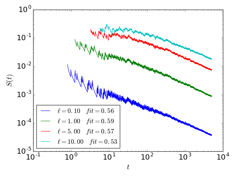
For a perfect circle $S(t)=0$, whereas $S(t)>0$ estimates the ‘rugosity’ of the system. The results shown in Fig. 8(top) indicate that for $\theta=0$, $S(t)$ is larger than zero but tends to zero for large values of $t$ as expected from the previous discussion and the model $M_{0}$ seems to be a sound approximation when $\theta=0$. But, for $\theta=1$, this is not true anymore: we observe in Fig. 8(bottom) that $S(t)>1$ and that $S(t)$ tends to a constant for large $t$, consistently with the previous results.

Figure 8: (Left) Example of shapes obtained for the primary colony in the $M_{1}$ model. (Top-left) Case $\theta=0$, $\ell=10$. (Top-right) Case $\theta=1$, $\ell=2$. (right) $S(t)$ versus $t$. On the top we have the behavior for $\theta=0$ averaged over $10$ simulations and on the bottom $\theta=1$ averaged over $100$ simulations.

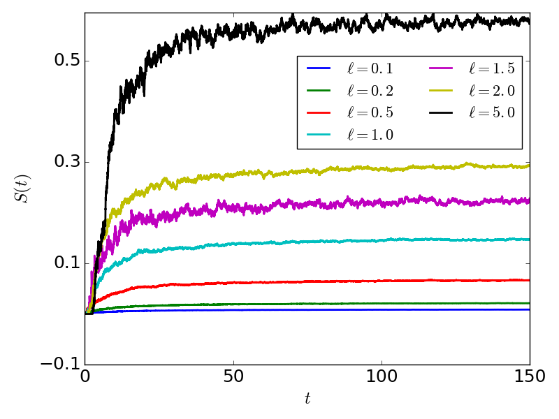We developed the general framework allowing the theoretical discussion of the growth and coalescence process. We discussed the quantitative predictions for the simpler model in which the emission rate depend on the exponent $\theta$, while the distance $\ell$ is constant and the process is isotropic. However, it is possible to integrate other specific features such as anisotropy or random emission distances and to investigate how these latter modify the actual results. Also, the circular approximation that allows for this analytical approach seems to be justified in cases where the emission rate grows not too quickly with the size of the primary colony. Otherwise, it is necessary to take the geometry of the colony into account, and making the theoretical extremely challenging. This model is very general and versatile, the results obtained are potentially useful to gain insights into the understanding of population proliferation, tumor growth and is also of great interest for modeling the dynamics of complex systems such as the sprawl of cities.

Acknowledgments

GC thanks the Complex Systems Institute in Paris (ISC-PIF) for hosting her during part of this work and for providing the OpenMole platform. MB thanks the city of Paris for its funding ‘Paris 2030’.

Supplementary material

The model $M_{0}$: further investigations

We discuss for $\theta>1$ the range of validity of the power-law behavior $r(t)\sim t^{\beta}$ , exploring the second order behavior.
Assuming the following form for the evolution of the radius of the primary colony with time,

$$r(t)\sim at^{\beta}+bt^{\beta^{\prime}}~{},$$ (25)

we consider the simplified Shigesada-Kawasaki system of equations given by

$$\frac{dr}{dt} =c+\frac{\lambda_{0}r^{\theta-1}}{2}x(t)^{2}~{},$$ (26)

$$x(t) =\frac{\ell_{0}}{1+\frac{\dot{r}}{c}}~{};$$ (27)

with $A=\frac{\lambda}{2}c^{2}\ell_{0}^{2}$. After some calculations, a development at the first and second order of Eq. (26) bring to the following results

$$\beta^{\prime}=1~{},$$ (28)

$$a=\left(\frac{2\beta^{3}}{{\ell}_{0}^{2}\lambda_{0}c^{2}}\right)^{\frac{1}{\theta-4}}~{},$$ (29)

and

$$b=\frac{4-\theta}{15-6\theta}~{}.$$ (30)

Being all the parameters determined we can deduce the value of the time $t_{min}=(b/a)^{1/(\beta-1)}$ starting from which the second order term begins to be smaller than the first order one. Hence, for $t\gg t_{min}$ we can write $r(t)\sim at^{\beta}$, neglecting the second order term. After some calculation one gets

$$t_{min}=f(\theta)\left(\frac{2c^{2-\theta}}{{\lambda}_{0}{\ell_{0}}^{2}}\right)^{\frac{1}{\theta-1}}$$ (31)

with

$$f(\theta)=\left(\frac{4-\theta}{15-6\theta}\right)^{\frac{4-\theta}{\theta-1}}\left(\frac{27}{(4-\theta)^{3}}\right)^{\frac{1}{\theta-1}}~{}.$$ (32)

We remark moreover that the Shigesada-Kawasaki equations are valid only if the coalescence of a colony does not cause the coalescence of another secondary colony. This means that the increasing in the radius at time $t$, $\delta r(t)$ has to be smaller than the distance between two successively emitted secondary colonies. The following relation has to be verified

$$\sqrt{r^{2}+{x^{*}}^{2}}-r<\frac{2c}{\lambda_{0}r^{\theta}}~{}.$$ (33)

From Eq. (27) one can write

$$x(t)\simeq\frac{c\ell_{0}}{\dot{r(t)}}~{},$$ (34)

this implies the following relation

$$x(t)\sim dt^{-\alpha}$$ (35)

with $\alpha=\beta-1$ and $d=c\ell_{0}/(\beta a)$. After some calculations one can show that the Shigesada-Kawasaki system of equations is valid only for $t<t_{max}$, with

$$t_{max}=g(\theta)\left(\frac{2c^{2-\theta}}{{\lambda}_{0}{\ell_{0}}^{2}}\right)^{\frac{1}{\theta-1}}$$ (36)

and

$$g(\theta)=2^{\frac{4-\theta}{\theta-1}}\beta~{}.$$ (37)

To summarize, we are able to observe the power-law behavior given by $r(t)\sim t^{\beta}$ in the range of time for which $t_{min}\ll t<t_{max}$. The size of the range of validity depends on the ratio between $g(\theta)$ and $f(\theta)$. This ratio decreases when $\theta$ increases as shown in Fig. 9.

Figure 9: $g(\theta)/f(\theta)$ versus $\theta$.

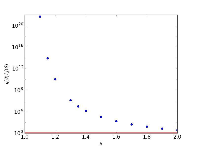
In the table 1 we report for different $\theta$, the values of the variable $\eta^{2}\lambda_{0}/2$ for which we performed numerical simulations and fit, and the corresponding values of $t_{min}$, $t_{max}$.

	$\theta=1.1$	$\theta=1.2$	$\theta=1.3$	$\theta=1.4$	$\theta=1.6$	$\theta=2.0$
$\frac{\eta^{2}\lambda_{0}}{2}$	$0.5$	$0.8$	$2.2$	$2.2$	$5$	$20$
$t_{min}$	$3\times 10^{-16}$	$5\times 10^{-7}$	$6\times 10^{-3}$	$5\times 10^{-2}$	$1.74$	$30$
$t_{max}$	$1.5\times 10^{6}$	$5.7\times 10^{3}$	$8.1\times 10^{3}$	$7.7\times 10^{2}$	$2.9\times 10^{2}$	$1.2\times 10^{2}$

Table 1: In the table we report for the different $\theta$, the values of the variable $\eta^{2}\lambda_{0}/2$ for which we performed the fit, and the corresponding values of $t_{c}$, $t_{max}$.

Avalanche effect

We have just discussed that it exists a time $t_{max}$ over which the Shigesada-Kawasaki equations are not valid anymore. Indeed, for $t>t_{max}$ avalanche effects arise.

Figure 10: (Top) $n_{a}$ vs. $t$ (Middle) $n_{c}$ vs. $t$. (Bottom) $r(t)$ vs. $t$. The results are obtained averaging over $100$ simulations. For $\theta=1.4$, $\ell=50$, $c=1$, $\lambda=0.001$.

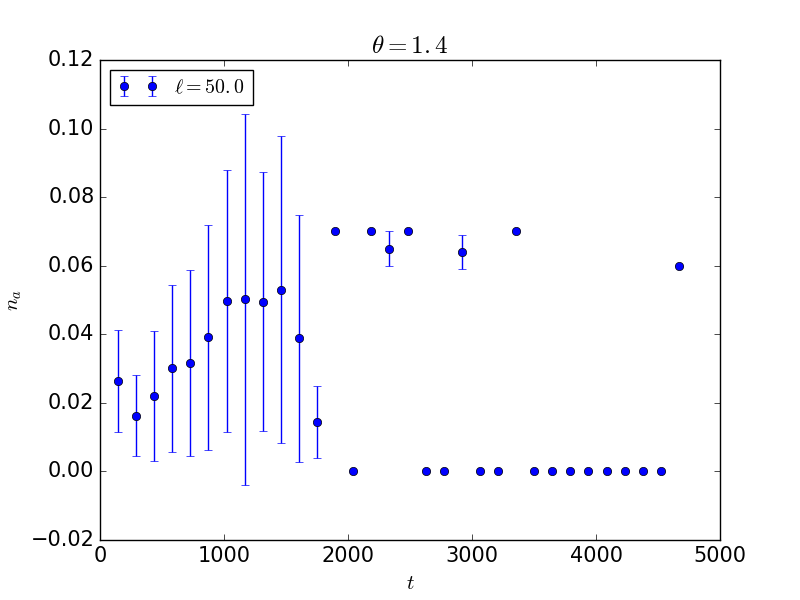
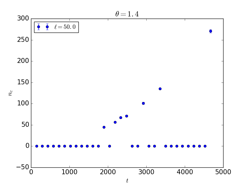
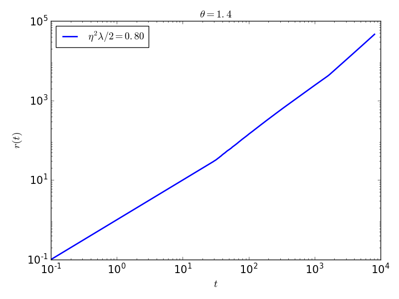
This is due to the high emission rate and means that not only we can have multiple coalescences, (that is more colonies absorbed in a single time step), but the increase in the radius produced by these coalescences can bring to other coalescences before moving to the next time step. Every time this happens we say that we observe an avalanche. In this situation the Shigesada-Kawasaki equations do not held and another treatment of the problem is necessary. This goes beyond the aim of this paper, however we performed numerical simulations to highlight this phenomenon, with the choice of $\theta=1.4$. At each time step $dt=0.001$ we count the number of avalanches $n_{a}$ and the number of total coalescences $n_{c}$ happened during $dt$ as consequence of the different avalanches.
The plots are shown in Fig. 10(a-b) where we observe that at a given time around $t\approx 2000$, the avalanche phenomenon change behavior acquiring more relevance, and bringing to a change in the slope characterizing the behavior of $r(t)$ with time (see Fig. 10-c).

The $M_{1}$ model: further empirical results

Case $\theta=0$

We present here further simulation results obtained for the $M_{1}$ model with a constant emission rate $\lambda(r)=\lambda_{0}$.

Figure 11: (Top) $A(t)$ vs. $t$. (Bottom) $P(t)$ vs. $t$. For different values of $\ell$ we plot in a log-log scale, the area and the perimeter of the primary colony versus time averaged over $10$ simulations. We perform a power-law fit and the values of the exponents obtained are shown in the insets.

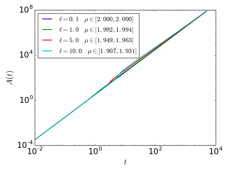
We assume that the area $A$ and the perimeter $P$ of the primary colony obey to a power-law scaling of the form

$$A(t)\sim t^{\mu}\qquad P(t)\sim t^{\nu}~{}.$$ (38)

In Fig. 11 we perform a power-law fit on the empirical results for two different time regimes. This allows us to examine eventual finite-size effects: we choose $t>t_{fc}$ and then $t>100t_{fc}$, with $t_{fc}$ being the time at which the first coalescence happens. The values of the exponents $\mu$ and $\nu$ are shown in the insets of Fig. 11, with the higher value corresponding to the choice $t>100t_{fc}$.

We assume that the sub-dominant corrections are described by the scaling forms

$$\frac{A(t)}{\pi c^{2}t^{2}}-1\sim t^{-\gamma}\qquad\quad\frac{P(t)}{2\pi ct}-1\sim t^{-\gamma^{\prime}}~{}.$$ (39)

In the Table 2 we report for the different choice of $\ell$, the values of $t^{*}$ and of the exponents $\gamma$ and $\gamma^{\prime}$. For each value of $\ell$ the smaller value of the exponent correspond to the fit for $t>t^{*}$ and the larger value to the fit range $t>10t^{*}$.

	$\ell=0.10$	$\ell=1.0$	$\ell=5.0$	$\ell=10.0$
$\gamma$	$0.53-0.53$	$0.55-0.57$	$0.54-0.56$	$0.52-0.54$
$\gamma^{\prime}$	$0.54-0.55$	$0.56-0.58$	$0.55-0.58$	$0.53-0.55$
$t^{*}$	$10$	$30$	$70$	$100$

Table 2: In the table we report for the different choice of $\ell$, the values of $t^{*}$ and of the exponents $\gamma$ and $\gamma^{\prime}$. For each value of $\ell$ the smaller value of the exponent correspond to the fit for $t>t^{*}$ and the larger value to the fit range $t>10t^{*}$.

Case $\theta=1$

The simulations results for the area $A(t)$ and the perimeter $P(t)$ of the primary colony, obtained for different values of $\ell$ are shown in Fig. 12. We assume the power-law behaviors given by Eq. (38) and we perform a fit on the empirical data. The values of the exponents obtained (for the time range $t>t_{fc}$ and $t>20t_{fc}$, with $t_{fc}$ the time at which the first coalescence happens) are shown in the insets of Fig. 12. The higher values correspond to the choice $t>20t_{fc}$ and this suggests that, taking possible finite-size effects into account, one can write

$$\mu\approx 2\qquad\nu\approx 1~{}.$$ (40)

Figure 12: (Top) $A(t)$ vs. $t$. (Bottom) $P(t)$ vs. $t$. For different values of $\ell$ we plot in a log-log scale, the area and the perimeter of the primary colony versus time averaged over $100$ simulations. We perform a power-law fit and the values of the exponents obtained are shown in the insets.

References

- (1) N. Shigesada and K. Kawasaki, Invasion by stratified diffusion (Oxford University Press, USA, 1997), chap. 5, p. 79103.
- (2) J. Clark, M. Lewis, and H. L., The American Naturalist, 157, 537 (2001).
- (3) K. Iwata, K. Kawasaki, and N. Shigesada, J. theor. Biol. 203, 177 (2000).
- (4) V. Haustein and U. Schumacher, J. Clin. Bioinforma. 2 (2012).
- (5) M. Barthelemy, The Structure and Dynamics of Cities (Cambridge University Press, 2016).
- (6) S. Angel, S. Sheppard, D. L. Civco, R. Buckley, A. Chabaeva, L. Gitlin, A. Kraley, J. Parent, and M. Perlin, The dynamics of global urban expansion (World Bank, Transport and Urban Development Department Washing- ton, DC, 2005).
- (7) R. A. Fisher, Annals of Human Genetics 7, 355 (1937).
- (8) N. Shigesada and K. Kawasaki, Invasion and the range expansion of species: effects of long-distance dispersal (Blackwell Science, 2002), chap. 17, p. 350373.
- (9) M. Lewis, S. Petrovskii, and J. Potts, The Mathematics Behind Biological Invasions (Springer International Publishing, 2016).