NLO and off-shell effects in top quark mass determinations

Abstract

We study the impact of different theoretical descriptions of top quark pair production on top quark mass measurements in the di-lepton channel. To this aim, the full NLO corrections to $pp\rightarrow W^{+}W^{-}b\bar{b}\rightarrow(e^{+}\nu_{e})\,(\mu^{-}\bar{\nu}_{\mu})\,b\bar{b}$ production are compared to calculations in the narrow width approximation, where the production of a top quark pair is calculated at NLO and combined with three different descriptions of the top quark decay: leading order, next-to-leading order and via a parton shower. The different theory predictions then enter the calibration of template fit functions, which are used for a fit to pseudo-data. The offsets in the top quark mass resulting from the fits based on the various theoretical descriptions are determined.

1 Introduction

The top quark mass is one of the most important parameters in the Standard Model (SM). As the top quark features the largest Yukawa coupling, it is closely linked to Higgs physics. Furthermore, the Higgs potential and therefore the vacuum stability of the SM depends critically on the value of the top quark mass. Processes involving top quarks allow for important precision tests of the SM and appear amongst the dominant backgrounds for many New Physics searches. They also allow to further constrain the gluon PDF at large $x$-values Czakon:2013tha ; Guzzi:2014wia ; delDuca:2015gca ; Czakon:2016olj .

The measurement of the top quark mass is complicated due to the fact that the reconstruction of $t\bar{t}$ events from complex hadronic and leptonic final states is an arduous task. Measurements of the top quark mass have been performed in various channels by the Tevatron and LHC collaborations, where the latest combinations can be found in Refs. CDF-1402 ; Abazov:2017ktz ; ATLAS-CONF-2017-071 ; Khachatryan:2015hba . While the most precise result in the di-lepton channel has an uncertainty of $0.84\mathrm{\>GeV}$ Aaboud:2016igd , the most precise combined results for the top quark mass achieve a precision of about $0.5\mathrm{\>GeV}$ Khachatryan:2015hba ; ATLAS-CONF-2017-071 . The precision achieved nowadays is the result of joint efforts in the experimental as well as the theory community to reduce the systematic uncertainties inherent to top quark mass measurements. For recent theoretical studies with regards to the definition and extraction of the top quark mass, see e.g. Frixione:2014ala ; Beneke:2016cbu ; Butenschoen:2016lpz ; Kawabata:2016aya ; Hoang:2017suc ; Hoang:2017btd ; Hoang:2017kmk ; Bevilacqua:2017ipv ; Nason:2017cxd ; Corcella:2017rpt ; Ravasio:2018lzi ; Hoang:2018ned .

The theoretical description of top quark pair production at hadron colliders has improved substantially in recent years. For stable top quarks, NNLO corrections to differential distributions are known Czakon:2015owf ; Czakon:2016dgf ; Czakon:2017dip and have recently been combined with NLO electroweak corrections Czakon:2017wor . The impact of electroweak corrections on distributions related to $t\bar{t}$ production has been studied in Refs. Hollik:2011ps ; Kuhn:2013zoa ; Pagani:2016caq for on-shell top quarks, and in Ref. Denner:2016jyo for both the on-shell case and with complete off-shell effects. Electroweak corrections to multi-jet merged on-shell top quark pair production have been calculated in Ref. Gutschow:2018tuk . Due to their very high complexity, the NNLO fixed-order calculations have so far only been combined with top quark decays in the narrow-width approximation (NWA), which factorises the production and decay processes. Radiative corrections to top quark decays have been calculated in Refs. Bernreuther:2004jv ; Melnikov:2009dn ; Campbell:2012uf , and since have been extended up to NNLO QCD Brucherseifer:2013iv ; Gao:2017goi . Resummation also has been accomplished up to NNLL, together with other improvements going beyond fixed order Beneke:2011mq ; Cacciari:2011hy ; Ferroglia:2013awa ; Broggio:2014yca ; Kidonakis:2015dla ; Pecjak:2016nee .

However, a description of top quark pair production and decay which predicts the shapes of distributions with an accuracy required for improvements on the current experimental precision needs to go beyond the narrow-width approximation. NLO QCD calculations of $W^{+}W^{-}b\bar{b}$ production, including leptonic decays of the $W$ bosons, have been performed in Refs. Denner:2010jp ; Denner:2012yc ; Bevilacqua:2010qb ; Heinrich:2013qaa . These calculations use the 5-flavour scheme, where the $b$-quarks are treated as massless partons. In Ref. Heinrich:2013qaa , particular emphasis has been put on the impact of the non-factorising contributions on the top quark mass measurements. Recently the calculation of the NLO QCD corrections to $W^{+}W^{-}b\bar{b}$ production with full off-shell effects has also been achieved in the lepton plus jets channel Denner:2017kzu .

The $b$-quark mass effects on observables like the invariant mass of a lepton-$b$-quark pair ($m_{lb}$) are very small. However, the use of massive $b$-quarks (more precisely, the 4-flavour scheme, 4FNS) has the (technically) important feature that it avoids collinear singularities due to $g\to b\bar{b}$ splittings. This implies that any phase space restrictions on the $b$-quarks can be made without destroying infrared safety, and thus allows to consider 0, 1- and 2-jet bins for $pp\to e^{+}\nu_{e}\mu^{-}\bar{\nu}_{\mu}b\bar{b}$ in one and the same setup, which is important for cross sections defined by jet vetos. In Refs. Frederix:2013gra ; Cascioli:2013wga , NLO calculations in the 4FNS have been performed.

The next step in complexity towards a realistic description of the measured final states consists in combining fixed-order calculations with a parton shower. The effect of radiative corrections to both, production and decay, in the factorised approach matched to a parton shower has been investigated in Ref. Campbell:2014kua within an extension of the PowHeg Nason:2004rx ; Frixione:2007vw ; Alioli:2010xd framework, called ttb_NLO_dec in the POWHEG-BOX-V2. Within the Sherpa framework, NLO QCD predictions for top quark pair production with up to three jets matched to a parton shower are also available, see Refs. Hoeche:2014qda ; Hoche:2016elu . A new NLO multi-jet merging algorithm relevant to top quark pair production is also available in Herwig 7.1 Bellm:2017idv .

Based on an NLO calculation of $W^{+}W^{-}b\bar{b}$ production combined with the Powheg framework, first results of the $W^{+}W^{-}b\bar{b}$ calculation in the 5-flavour scheme matched to a parton shower have been presented in Ref. Garzelli:2014dka . However, it has been noticed later that the matching of NLO matrix elements involving resonances of coloured particles to parton showers poses problems which can lead to artefacts in the top quark lineshape Jezo:2015aia . As a consequence, an improvement of the resonance treatment has been implemented in POWHEG-BOX-RES, called “resonance aware matching”, and combined with NLO matrix elements from OpenLoops Cascioli:2011va , to arrive at the most complete description so far Jezo:2016ujg , based on the framework developed in Ref. Jezo:2015aia and the 4FNS calculation of Ref. Cascioli:2013wga . An alternative algorithm to treat radiation from heavy quarks in the Powheg NLO+PS framework has been presented in Ref. Buonocore:2017lry . An improved resonance treatment in the matching to parton showers for off-shell single top production at NLO has been worked out in Refs. Jezo:2015aia ; Frederix:2016rdc , and similarly for off-shell $t\bar{t}$ and $t\bar{t}H$ production in $e^{+}e^{-}$ collisions in Ref. Nejad:2016bci .

In this paper, we investigate the impact of different approximations on the top quark mass measurement simulating a concrete experimental setup. In particular, we follow up on an open question raised in Ref. Heinrich:2013qaa , where we performed a study of NLO effects in top quark mass measurements based on the observable $m_{lb}$ in the framework of a top quark mass measurement as performed by ATLAS using the template method Aad:2015nba ; Aaboud:2016igd . Substantial distortions in the $m_{lb}$ distribution are induced by scale variations calculated by including the full NLO corrections to the $W^{+}W^{-}b\bar{b}$ final state (with leptonic $W$-decays). On the other hand, in the factorised approach, where the $t\bar{t}$ cross section calculated at NLO is combined with LO top quark decays in the NWA, the shape distortions due to the scale variations are minor. As the experimental analysis is based on normalised distributions, the shape differences induced by scale variations translate in a very sensitive manner into the theoretical uncertainties on the extraction of the top quark mass.

The question arises where the shape changes come from, i.e. whether they mainly come from the non-factorisable contributions contained in the full NLO corrections to $W^{+}W^{-}b\bar{b}$, or from factorisable NLO corrections to the top quark decay. And, if the latter is true, what is the effect of a parton shower in combination with the factorised approach, as it should contain the leading contributions of the NLO corrections to the top quark decay. To answer these questions, we compare the NLO calculation of $W^{+}W^{-}b\bar{b}$ production of Ref. Heinrich:2013qaa with the calculation based on the narrow-width approximation where both $t\bar{t}$ production and decay are calculated at NLO, as described in Ref. Melnikov:2009dn . We further quantify the impact of a parton shower in the narrow-width approximation, combining the NLO matrix elements of top quark pair production with Sherpa Gleisberg:2008ta .

The structure of this paper is as follows. In Section 2, we describe our different calculations performed to compare theoretical descriptions of the complex final state of two charged leptons, two $b$-jets and missing energy. In Section 3, we compare these different theoretical descriptions for a number of observables relevant to top quark mass measurements. We then quantify in Section 4 how the differences in the theoretical descriptions impact a template fit as utilised in experimental determinations of the top quark mass, before we conclude in Section 5.

2 The different stages of the theoretical description

We study the following descriptions of top quark pair production in the di-lepton channel:

     $\mathbf{NLO_{full}}$:

full NLO corrections to $pp\to W^{+}W^{-}b\bar{b}$ with leptonic $W$-decays,

     $\mathbf{NLO_{NWA}^{NLOdec}}$:

NLO $t\bar{t}$ production $\otimes$ NLO decay,

     $\mathbf{NLO_{NWA}^{LOdec}}$:

NLO $t\bar{t}$ production $\otimes$ LO decay,

     $\mathbf{NLO_{PS}}$:

NLO $t\bar{t}$ production+shower $\otimes$ decay via parton showering.

We furthermore use the abbreviation $\mathbf{LO_{full}}$ for $W^{+}W^{-}b\bar{b}$ calculated at leading order, the abbreviation $\mathbf{LO_{NWA}^{LOdec}}$ for LO $t\bar{t}$ production $\otimes$ LO decay and the abbreviation $\mathbf{LO_{PS}}$ for LO $t\bar{t}$ production $\otimes$ decay via parton showering. We investigate the effects of different levels in the description of the top quark decay, isolating the latter from the effects of the non-resonant and non-factorisable contributions contained in the $\mathrm{NLO_{full}}$ calculation. This is done by emulating a concrete experimental analysis used for top quark mass determinations. As we match to a parton shower only in combination with LO top quark decays, we do not need to address the problem of “resonance-aware matching” Jezo:2016ujg ; Frederix:2016rdc . This allows us to get a clear idea of the effects of the various approximations used here, which in turn can serve as a basis for future studies entirely relying on showered results.

The calculations $\mathrm{NLO_{full}}$ and $\mathrm{NLO_{NWA}^{LOdec}}$ have been already described in detail in Ref. Heinrich:2013qaa . Here we briefly summarise only the main features. We use GoSam Cullen:2011ac ; Cullen:2014yla plus Sherpa Gleisberg:2008ta , version 2.2.3, where the virtual corrections generated by GoSam are linked to Sherpa via the Binoth-Les-Houches-interface Binoth:2010xt ; Alioli:2013nda . This applies not only to the calculations $\mathrm{NLO_{full}}$ and $\mathrm{NLO_{NWA}^{LOdec}}$ but also to the $\mathrm{NLO_{PS}}$ computation. We note that our full NLO calculation of the process $pp\rightarrow W^{+}W^{-}b\bar{b}\rightarrow(e^{+}\nu_{e})\,(\mu^{-}\bar{\nu}_{\mu})\,b\bar{b}$ provides a complete description of the final state including singly-resonant and non-resonant top quark contributions. Example diagrams are shown in Fig. 1. The computation relies on the 5-flavour scheme, i.e. the $b$-quark is treated as massless. To take the top quark decay width into account in a gauge invariant way, the complex mass scheme Denner:2006ic is used. In our setup, this entails a replacement of the top quark mass by a complex number $\mu_{t}$ evaluated according to

$$\mu_{t}^{2}\;=\;m_{t}^{2}-i\,m_{t}\,\Gamma_{t}~{}.$$ (1)

The $W$-bosons and intermediate $Z$-bosons also have complex masses due to their widths. Note that we only consider resonant $W$-boson decays.

Figure 1: Examples of one-loop Feynman diagrams contributing to the $\mathrm{NLO_{full}}$ calculation, i.e. the full $W^{+}W^{-}b\bar{b}$ calculation at NLO: two diagrams are shown depicting a non-resonant (left) and a non-factorisable virtual contribution (right).

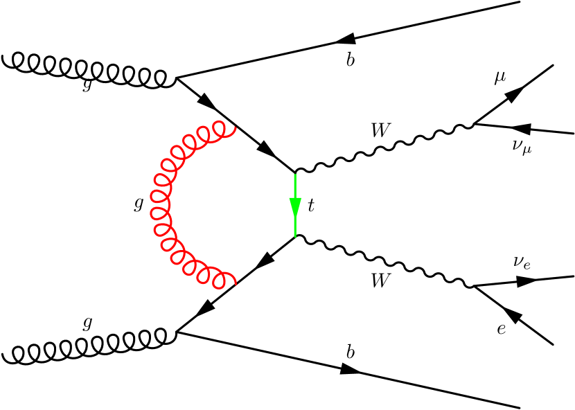
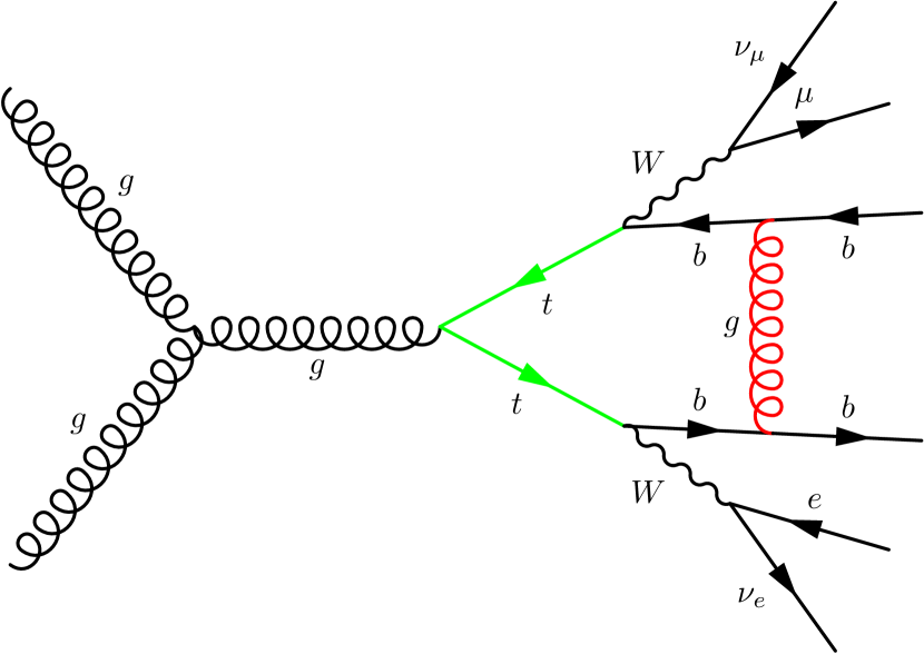
The results for the $\mathrm{NLO_{NWA}^{NLOdec}}$ calculation are obtained as described in Ref. Melnikov:2009dn . This framework relies on the factorisation of the matrix elements according to

$$\mathcal{M}^{\mathrm{NWA}}_{ij\to t\bar{t}\to b\bar{b}2l2\nu}\;=\;\mathcal{P}_{ij\to t\bar{t}}\otimes\mathcal{D}_{t\to bl^{+}\nu}\otimes\mathcal{D}_{\bar{t}\to\bar{b}l^{-}\bar{\nu}}~{},$$ (2)

where $\mathcal{P}_{ij\to t\bar{t}}$ describes the $t\bar{t}$ production process and $\mathcal{D}_{t\to bl\nu}$ the top quark decay dynamics. Spin correlations are included as indicated by the symbol $\otimes$. Squaring Eq. (2) and integrating over the phase space yields the double-resonant partonic cross section

$$\hat{\sigma}_{ij\to b\bar{b}2l2\nu}\;=\;\int\!\!\mathrm{d}\mathrm{PS}\;|\mathcal{M}^{\mathrm{NWA}}_{ij\to t\bar{t}\to b\bar{b}2l2\nu}|^{2}+\mathcal{O}\left(\Gamma_{t}\big{/}m_{t}\right)$$ (3)

where off-shell effects are parametrically suppressed by $\Gamma_{t}\big{/}m_{t}\approx 0.7\%$. Expanding Eq. (2) up to NLO yields

$$\mathcal{M}^{\mathrm{NWA,\;NLO}}_{ij\to t\bar{t}\to b\bar{b}2l2\nu}= \mathcal{P}_{ij\to t\bar{t}}^{\mathrm{LO}}\otimes\mathcal{D}^{\mathrm{LO}}_{t\to bl^{+}\nu}\otimes\mathcal{D}^{\mathrm{LO}}_{\bar{t}\to\bar{b}l^{-}\bar{\nu}}+\mathcal{P}_{ij\to t\bar{t}}^{\delta\mathrm{NLO}}\otimes\mathcal{D}^{\mathrm{LO}}_{t\to bl^{+}\nu}\otimes\mathcal{D}^{\mathrm{LO}}_{\bar{t}\to\bar{b}l^{-}\bar{\nu}}$$

$$+ \mathcal{P}_{ij\to t\bar{t}}^{\mathrm{LO}}\otimes\left(\mathcal{D}^{\delta\mathrm{NLO}}_{t\to bl^{+}\nu}\otimes\mathcal{D}^{\mathrm{LO}}_{\bar{t}\to\bar{b}l^{-}\bar{\nu}}+\mathcal{D}^{\mathrm{LO}}_{t\to bl^{+}\nu}\otimes\mathcal{D}^{\delta\mathrm{NLO}}_{\bar{t}\to\bar{b}l^{-}\bar{\nu}}\right)~{}.$$ (4)

The NLO corrections to the production process $\mathcal{P}_{ij\to t\bar{t}}^{\delta\mathrm{NLO}}$ involve the virtual and real emission matrix elements $\mathcal{M}_{gg/q\bar{q}\to t\bar{t}}^{\mathrm{virt}}$, $\mathcal{M}_{gg/q\bar{q}\to t\bar{t}+g}^{\mathrm{real}}$ and $\mathcal{M}_{qg/\bar{q}g\to t\bar{t}+q/\bar{q}}^{\mathrm{real}}$. The corresponding NLO decay parts are given by

$$\mathcal{D}^{\mathrm{virt(real)}}_{t\to bl\nu}\;=\;\frac{\mathcal{M}^{\mathrm{virt(real)}}_{t\to bW(+g)}}{\sqrt{2m_{t}\Gamma_{t}^{\mathrm{NLO}}}}\otimes\frac{\mathcal{M}_{W\to l\nu}}{\sqrt{2M_{W}\Gamma_{W}^{\mathrm{NLO}}}}~{}.$$ (5)

We note that, in contrast to Ref. Melnikov:2009dn , the top quark width $\Gamma_{t}^{\mathrm{NLO}}$ in the denominator is not expanded as $(\Gamma_{t}^{\mathrm{NLO}})^{-1/2}=(\Gamma_{t}^{\mathrm{LO}})^{-1/2}\left(1-1/2\,\alpha_{s}\,\Gamma_{t}^{\delta\mathrm{NLO}}/\Gamma_{t}^{\mathrm{LO}}\right)$, analogously for $(\Gamma_{W}^{\mathrm{NLO}})^{-1/2}$.

For our studies relying on $\mathrm{NLO_{NWA}^{LOdec}}$ results, we remove all contributions in the second line of Eq. (2) and use $\Gamma_{t,W}^{\mathrm{LO}}$ instead of $\Gamma_{t,W}^{\mathrm{NLO}}$. This treatment guarantees that $\int\!\mathrm{d}\mathrm{PS}\;|\mathcal{D}_{t\to bl\nu}|^{2}=\mathrm{BR}(t\to bl\nu)$ at LO and NLO, with $\mathrm{BR}(t\to bl\nu)$ denoting the branching ratio for the top quark decay.

Finally, the $\mathrm{NLO_{PS}}$ computations are based on the NLO plus parton-shower matching scheme as implemented in Sherpa Hoeche:2011fd . The original scheme was extended in Ref. Hoeche:2013mua to incorporate heavy-quark mass effects. Utilising this scheme, we obtain an NLO+PS accurate description of $t\bar{t}$+jets, or, in other words, the NLO description of the $t\bar{t}$ production shower. The top quark decays are attached afterwards such that LO spin correlations are preserved, and each decay configuration is supplemented by its respective decay shower following the same procedure as described in Ref. Hoche:2014kca . For our investigations, we used Sherpa version 2.2.3. In the course of this work, it was found that this version treats radiation emerging from top quark decays in resonant top quark processes in the same manner as radiation arising from continuum production processes. This resulted in an omission of the initial-state spectator mass term that suppresses the ordinary eikonal radiation of continuum initial-final dipoles. The problem has been identified and solved by the implementation of a dedicated dipole-shower algorithm for the decays, similar to Ref. Hamilton:2006ms . The patch implementing these changes has been provided by the Sherpa authors and was used for our results presented below. It will be made available on the corresponding software download pages, and included in the Sherpa program from version 2.2.5 onwards.

3 Phenomenological study of observables sensitive to the top quark mass

3.1 Definition of the observables

We study the following observables:

• $m_{lb}$ – which we define using the invariant mass squared

  $$m_{lb}^{2}\;=\;(p_{l}+p_{b})^{2}$$ (6)

  where $p_{l}$ denotes the four-momentum of the lepton and $p_{b}$ the four-momentum of the $b$-jet. As there are two top quarks, there are also two possible $m_{lb}$ values per event. Since experimentally, it is not possible to reconstruct the $b$-quark charge on an event-by-event basis with sufficient accuracy, one also needs a criterion to assign a pair of a charged lepton and a $b$-jet as the one stemming from the same top quark decay. Following Aaboud:2016igd , the algorithm applied here is to choose that $(l^{+}b\text{-jet},\,l^{-}b\text{-jet}^{\prime})$ pairing which minimises the sum of the two $m_{lb}$ values per event. Finally, the $m_{lb}$ observable used in the analysis is the mean of the two $m_{lb}$  values per event obtained when applying the above procedure.

• $m_{T2}$ – which corresponds to the kinematic variable $m_{T2}$ Lester:1999tx ; Barr:2003rg that, applied to the $b\bar{b}2l2\nu$ final state, is defined as

  $$m_{T2}^{2}\;=\;\min_{\mathbf{p}_{T}^{\nu_{1}}+\mathbf{p}_{T}^{\nu_{2}}=\mathbf{p}_{T}^{\mathrm{miss}}}\left[\max\left\{m_{T}^{2}\left(\mathbf{p}_{T}^{(lb)_{1}},\mathbf{p}_{T}^{\nu_{1}}\right),m_{T}^{2}\left(\mathbf{p}_{T}^{(lb)_{2}},\mathbf{p}_{T}^{\nu_{2}}\right)\right\}\right].$$ (7)

  Again the pairing of leptons and $b$-jets which minimises $m_{(lb)_{1}}+m_{(lb)_{2}}$ is chosen. The transverse mass is given by

  $$m_{T}^{2}\left(\mathbf{p}_{T}^{(lb)_{i}},\mathbf{p}_{T}^{\nu_{i}}\right)=m_{(lb)_{i}}^{2}+2\left(E_{T}^{(lb)_{i}}E_{T}^{\nu_{i}}-\mathbf{p}_{T}^{(lb)_{i}}\mathbf{p}_{T}^{\nu_{i}}\right)$$

  with $E_{T}=\sqrt{|\mathbf{p}_{T}|^{2}+m^{2}}$, where $m_{\nu_{i}}=0$ was used.

• $E_{T}^{\Delta R}$ – which is defined as

  $$E_{T}^{\Delta R}\;=\;\frac{1}{2}\,\left(E_{T}^{l_{1}}\Delta R(l_{1},b_{1})+E_{T}^{l_{2}}\Delta R(l_{2},b_{2})\right)$$ (8)

  using the above pairing criterion for leptons and $b$-jets.

We also consider the following fully leptonic observables, which are part of the set of observables used for a recent top quark mass determination from differential leptonic cross sections in Ref. ATLAS-CONF-2017-044 :

• $m_{ll}$ – as given by the invariant mass squared of the two charged leptons, defined as

  $$m_{ll}^{2}\;=\;(p_{l_{1}}+p_{l_{2}})^{2}~{}.$$ (9)

• $p_{T,\mu}$ – which is the transverse momentum of the muon.

• $\eta_{\mu}$ – which is the rapidity of the muon.

3.2 Input parameters and event requirements

We use the PDF4LHC15_nlo_30_pdfas sets Butterworth:2015oua ; Dulat:2015mca ; Harland-Lang:2014zoa ; Ball:2014uwa and a centre-of-mass energy of $\sqrt{s}=13\mathrm{\>TeV}$. Our default top quark mass is $m_{t}=172.5\mathrm{\>GeV}$. Leading order top quark and $W$ boson widths are used in the LO calculations and the NLO $t\bar{t}\,\otimes$ LO decay calculation, while NLO widths (Jezabek:1987nf, ) are used in the remaining NLO calculations. Widths at NLO appearing in propagators are not expanded in $\alpha_{s}$. The QCD coupling in the NLO widths is varied according to the chosen scale. For $\alpha_{s}$ evaluated at the central scale $m_{t}$, the numerical values for the widths are

$$\begin{matrix}\Gamma_{t}^{\mathrm{LO}}&=&1.4806\mathrm{\>GeV}{}&,&\quad\Gamma_{t}^{\mathrm{NLO}}&=&1.3535\mathrm{\>GeV}{},\\ \Gamma_{W}^{\mathrm{LO}}&=&2.0454\mathrm{\>GeV}{}&,&\quad\Gamma_{W}^{\mathrm{NLO}}&=&2.1155\mathrm{\>GeV}{},\\ \Gamma_{Z}&=&2.4952\mathrm{\>GeV}{}&.&&&\\ \end{matrix}$$ (10)

Jets are defined using the anti-$k_{T}$ algorithm Cacciari:2008gp as implemented in Fastjet Cacciari:2011ma , with $R=0.4$. For the electroweak parameters, we employ the following settings:

$$G_{\mu}\;=\;1.16637\cdot 10^{-5}\mathrm{\>GeV}{}^{-2},\quad M_{W}\;=\;80.385\mathrm{\>GeV}{},\quad M_{Z}\;=\;91.1876\mathrm{\>GeV}{}.$$ (11)

Inspired by Ref. Aaboud:2016igd , and taking into account the stronger trigger requirements for a $13\mathrm{\>TeV}$ analysis, the following list of event requirements is used. We require

• exactly two $b$-tagged jets with $p_{T}^{\mathrm{jet}}>25\mathrm{\>GeV}$ and $|\eta^{\mathrm{jet}}|<2.5$. Jets containing a $b\bar{b}$ pair are also defined as $b$-jets.

• exactly two oppositely charged leptons which fulfill $p_{T}^{\mu}>28\mathrm{\>GeV}$, $|\eta^{\mu}|<2.5$ for muons and $p_{T}^{e}>28\mathrm{\>GeV}$, $|\eta^{e}|<2.47$ for electrons excluding the range $1.37<|\eta^{e}|<1.52$. For both types of charged leptons with respect to any jet fulfilling the jet requirements, a separation of $\Delta R(l,\mathrm{jet})>0.4$ is required.

• $p_{T}^{lb}>120\mathrm{\>GeV}$. Using the same lepton $b$-jet assignments as for $m_{lb}$, the observable $p_{T}^{lb}$ denotes the mean transverse momentum of the two lepton–$b$-quark systems.

The $b$-quarks are treated as massless in all fixed-order calculations. We chose $\mu_{R}=\mu_{F}=m_{t}$ as our central scale. The impact of choosing $H_{T}/2$ (rather than $m_{t}$) as the central scale on the top quark mass determined by our method has been shown to be very small Heinrich:2013qaa . It furthermore would be difficult to facilitate an $H_{T}$ definition for the $\mathrm{NLO_{PS}}$ approach that matches the one used in the $\mathrm{NLO_{full}}$ calculation. Even a simplified $H_{T}$ definition that involved only the charged lepton and $b$-jet transverse momenta and neglected the neutrino momenta would be affected because the parton showering changes the $p_{T}$ spectrum of the final state particles. We therefore considered it more consistent to choose $m_{t}$ as the central renormalisation and factorisation scale throughout all calculations. The scale variation bands are obtained by varying $\mu_{R}$ and $\mu_{F}$ simultaneously by a factor of two and one half with respect to the central scale. We have also performed 7-point scale variations and found that the simultaneous variations always formed the most conservative uncertainty band in the $m_{lb}$ and $m_{T2}$ distributions, Figs. 2 and 3.

For the parton shower results, we have also investigated the impact of a dynamic scale, which we call $\mu_{t\bar{t}}$, to compute the matrix elements of the hard scattering processes producing the top quark pairs. The scale $\mu_{t\bar{t}}$ is a “colour flow inspired” QCD scale, introduced in Ref. Hoeche:2013mua . Using Mandelstam variables $s$, $t$ and $u$, it is defined as

$$\mu_{t\bar{t}}^{2}(q\bar{q}\to t\bar{t}) \;=\;2\,p_{q}p_{t}\;=\;m_{t}^{2}-t~{},$$

$$\mu_{t\bar{t}}^{2}(\bar{q}q\to t\bar{t}) \;=\;2\,p_{q}p_{t}\;=\;m_{t}^{2}-u~{},$$

$$\mu_{t\bar{t}}^{2}(gg\to t\bar{t}) \;=\;\left\{\begin{array}[]{ccl}m_{t}^{2}-t&&w_{1}\varpropto\,\frac{u-m_{t}^{2}}{t-m_{t}^{2}}+\frac{m_{t}^{2}}{m_{t}^{2}-t}\left\{\frac{4\,t}{t-m_{t}^{2}}+\frac{m_{t}^{2}}{s}\right\}\\ &\text{with weight}&\\ m_{t}^{2}-u&&w_{2}\varpropto\,\frac{t-m_{t}^{2}}{u-m_{t}^{2}}+\frac{m_{t}^{2}}{m_{t}^{2}-u}\,\left\{\frac{4\,u}{u-m_{t}^{2}}+\frac{m_{t}^{2}}{s}\right\}~{}.\end{array}\right.$$ (15)

The value for the $gg$ partonic process is chosen randomly according to the relative size of the two weights $w_{1}$ and $w_{2}$.

Scheme	Central scale $\mu_{i}$	Variations $\xi_{i}\,\mu_{i}$
$\mu_{F}\mu_{R}{\alpha^{\mathrm{PS}}_{s}}$	$\mu_{F}=\mu_{R}=\mu_{Q}^{\mathrm{prod}}=m_{t}$, $\mu_{R}^{\mathrm{PS}}=p_{T}^{\mathrm{emit}}$	$\xi_{R}=\xi_{F}=\xi_{R}^{\mathrm{PS}}=\{0.5,1.0,2.0\}$
	$\mu_{F}=\mu_{R}=\mu_{Q}^{\mathrm{prod}}=\mu_{t\bar{t}}$, $\mu_{R}^{\mathrm{PS}}=p_{T}^{\mathrm{emit}}$
$\mu_{F}\mu_{R}\mu_{Q}$	$\mu_{F}=\mu_{R}=\mu_{Q}^{\mathrm{prod}}=m_{t}$, $\mu_{R}^{\mathrm{PS}}=p_{T}^{\mathrm{emit}}$	$\xi_{R}=\xi_{F}=\{0.5,1.0,2.0\}$ and
		$\hphantom{\xi_{R}=\,}\xi_{Q}=\{\sqrt{2},1.0,1/\sqrt{2}\}$
$\mu_{F}\mu_{R}\mu_{Q}{\alpha^{\mathrm{PS}}_{s}}$	$\mu_{F}=\mu_{R}=\mu_{Q}^{\mathrm{prod}}=m_{t}$, $\mu_{R}^{\mathrm{PS}}=p_{T}^{\mathrm{emit}}$	$\xi_{R}=\xi_{F}=\xi_{R}^{\mathrm{PS}}=\{0.5,1.0,2.0\}$
		and $\xi_{Q}=\{\sqrt{2},1.0,1/\sqrt{2}\}$

Table 1: Summary of schemes employed to assess the scale variations in the $\mathrm{NLO_{PS}}$ case. In all cases, the decay shower starting scale is kept constant, as given by its default $\mu_{Q}^{\mathrm{dec}}=M_{W}/2$. Note that the local $p_{T}^{\mathrm{emit}}$ values (squared) of each parton branching serve as the argument of ${\alpha_{s}}$ in the evaluation of the shower kernels. The related variation, $\xi_{R}^{\mathrm{PS}}\,\mu_{R}^{\mathrm{PS}}$, has been realised through appropriate adjustments of the Sherpa parameters CSS_IS_AS_FAC and CSS_FS_AS_FAC.

The standard $\mu_{R}$ and $\mu_{F}$ variations that we employ for our fixed-order calculations are not fully appropriate to assess the theory uncertainties of the $\mathrm{NLO_{PS}}$ computations, as the showering depends on further scale and parameter choices. For our studies, it is interesting to vary $\mu_{Q}^{\mathrm{prod}}$ as well as $\mu_{Q}^{\mathrm{dec}}$, which are the parameters controlling the overall size of the resummation domains assigned to the $t\bar{t}$ production and top quark decay showers, respectively. Within these resummation domains, subsequent shower emissions are evaluated from the values taken by the ordering variable of the parton shower. We therefore also alter the strength of the parton shower emissions by variations of $\mu_{R}^{\mathrm{PS}}$, the scale entering the evaluation of the strong coupling ${\alpha_{s}}(\mu_{R}^{\mathrm{PS}})$ used in the shower kernels. For the Sherpa CSshower, the ordering variable is associated with the local $p_{T}^{\mathrm{emit}}$ scales of the individual branchings, which means $\mu_{R,k}^{\mathrm{PS}}\sim p_{T,k}^{\mathrm{emit}}$ for the $k$-th branching. For the combined variation of several $\mathrm{NLO_{PS}}$ parameters, we follow the principle of identifying the strongest and weakest shower option that one can possibly obtain from the given individual parameter ranges. This is supposed to lead to a conservative shower uncertainty estimate.

Our default variation in the $\mathrm{NLO_{PS}}$ case, denoted by $\mu_{F}\mu_{R}{\alpha^{\mathrm{PS}}_{s}}$, is a combination of simultaneously varying $\mu_{F},\mu_{R}$ and $\mu_{R}^{\mathrm{PS}}$ by a factor of two up and down, with central scale $m_{t}$. Alternative ways of uncertainty assessment include the variation of $\mu_{Q}^{\mathrm{prod}}$ and $\mu_{Q}^{\mathrm{dec}}$. The Sherpa default is to set $\mu_{Q}^{\mathrm{prod}}$ equal to the factorisation scale, while the starting scale of the decay shower is set to $\mu_{Q}^{\mathrm{dec}}=M_{W}/2$ and not varied. The different scale variation schemes, which are used by us in the $\mathrm{NLO_{PS}}$ case are summarised in Table 1. For each of the schemes shown in Table 1, the uncertainty bands are defined as the maximum deviation from the central prediction on either side.

3.3 Numerical predictions

3.3.1 Comparison of the different theoretical descriptions

	X=LO $\left[\mathrm{fb}\right]$	X=NLO $\left[\mathrm{fb}\right]$
$\mathbf{X_{full}}$	$\left(739.5\pm 0.3\right)^{+31.5\%}_{-22.4\%}$	$\left(914\pm 3\right)^{+2.1\%}_{-7.6\%}$
$\mathbf{X_{NWA}^{LOdec}}$	$\left(727.3\pm 0.2\right)^{+31.4\%}_{-22.3\%}$	$\left(1029\pm 1\right)^{+10.4\%}_{-11.5\%}$
$\mathbf{X_{NWA}^{NLOdec}}$	-	$\left(905\pm 1\right)^{+2.3\%}_{-7.7\%}$
$\mathbf{X_{PS}},\mu=m_{t}$	$\left(637.7\pm 0.9\right)^{+29.7\%}_{-21.0\%}$	$\left(886\pm 1\right)^{+8.5\%}_{-9.3\%}$
$\mathbf{X_{PS}},\mu=\mu_{t\bar{t}}$	$\left(499.7\pm 0.7\right)^{+27.6\%}_{-19.3\%}$	$\left(805.2\pm 0.9\right)^{+12.3\%}_{-10.9\%}$

Table 2: Fiducial cross sections in various approximations. The first uncertainty is the precision of the Monte Carlo phase space integration. The scale variation uncertainty obtained by simultaneously varying renormalisation and factorisation scales by a factor of two (superscript) and one half (subscript) is given in percent. For the parton shower results, the given scale uncertainties are obtained by using the variation prescription $\mu_{F}\mu_{R}{\alpha^{\mathrm{PS}}_{s}}$ as detailed in the text.

In this section, we compare four different NLO descriptions of the $(e^{+}\nu_{e})\,(\mu^{-}\bar{\nu}_{\mu})\,b\bar{b}$ final state for the observables described in Section 2. Some of the purely leptonic observables have also been used by the ATLAS collaboration for their recent top quark mass determinations based on $8\mathrm{\>TeV}$ data presented in Ref. ATLAS-CONF-2017-044 . Aiming to quantify the relative differences of the theoretical descriptions, which should only mildly depend on the centre-of-mass energy, we show results at the present LHC setting of $13\mathrm{\>TeV}$. The corresponding fiducial cross sections are summarised in Table 2. While the level of agreement between the fixed-order full and NWA calculations is as expected, considerably smaller cross sections are obtained for the parton shower calculations. Showering leads to a softening of the final state $b$-jets. In turn, a good fraction of them no longer satisfy the jet requirements, resulting in an event loss. The parton shower computation with $\mu=\mu_{t\bar{t}}$ leads to an even smaller fiducial cross section than the computation relying on $\mu=m_{t}$, which is a consequence of the fact that the $\mu_{t\bar{t}}$ scale is larger, and therefore the value for $\alpha_{s}$ is smaller. In both cases, however, the loss of events due to insufficiently energetic $b$-jets after parton showering is similar, and amounts to about 12%.

Figure 2: Normalised differential cross sections for the invariant mass $m_{lb}$ at the $13\mathrm{\>TeV}$ LHC for four different theoretical descriptions: $\mathrm{NLO_{full}}$, $\mathrm{NLO_{NWA}^{NLOdec}}$, $\mathrm{NLO_{NWA}^{LOdec}}$ and $\mathrm{NLO_{PS}}$. The ratios of all descriptions to $\mathrm{NLO_{full}}$ including its scale uncertainty band are also shown.

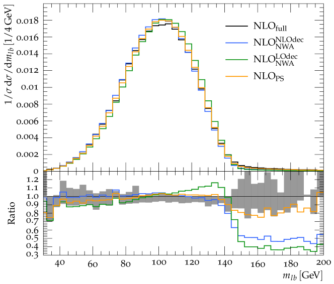
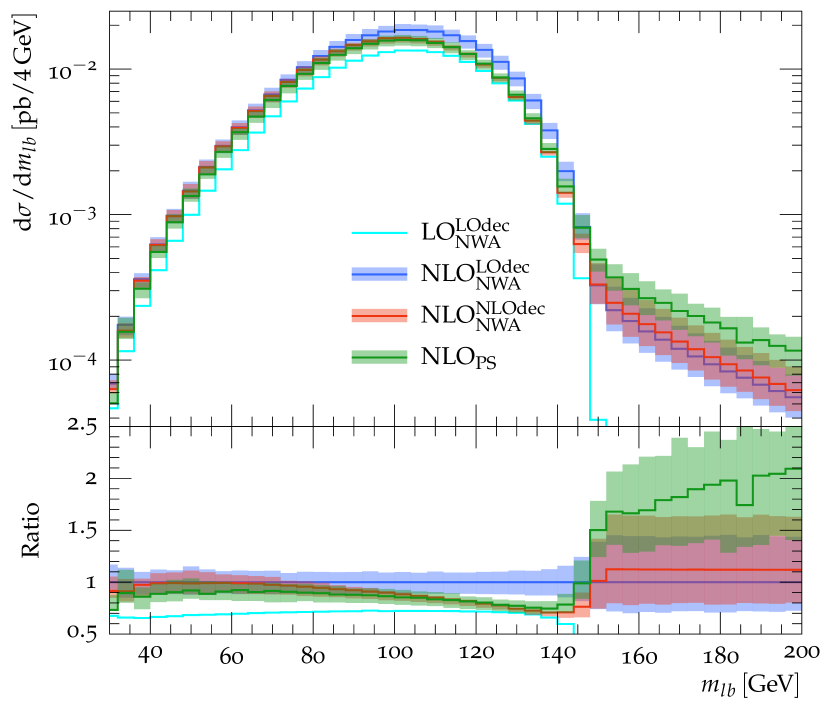
In Fig. 2, we present the normalised differential cross sections for $m_{lb}$ based on the four theoretical descriptions, evaluated at $\mu_{R}=\mu_{F}=m_{t}$. In the lower part of the figure, we show their ratio to the $\mathrm{NLO_{full}}$ prediction, including an uncertainty band from scale variations by a factor of two and one half with respect to the central scale. We find that 99% of the total fiducial cross section is accumulated in the range $40$–$150\mathrm{\>GeV}$. A kinematic edge at $m_{lb}^{\mathrm{edge}}=\sqrt{m_{t}^{2}-M_{W}^{2}}=152.6\mathrm{\>GeV}$ leads to a sharp drop in the distribution beyond which it is only populated by non-resonant contributions, additionally clustered radiation and incorrect $b$-lepton pairings. The significantly larger scale uncertainty for $m_{lb}\geq 150\mathrm{\>GeV}$ is due to the fact that NLO is the first non-trivial order populating this region. This conclusion is further substantiated by the sizeable perturbative correction that we discuss in the following section. Hence, resummation effects are expected to play a larger role in the vicinity of this kinematic boundary.

We now discuss the impact of off-shell and non-resonant contributions on the $m_{lb}$ distribution. Their effect is easiest seen by discussing $\mathrm{NLO_{NWA}^{NLOdec}}$, displayed in the lower part of Fig. 2. In the range $30\mathrm{\>GeV}\leq m_{lb}\leq 130\mathrm{\>GeV}$ this prediction agrees with the full calculation to within a few percent. The deviations are barely visible within the statistical fluctuations. Around the peak region of the differential cross section for $m_{lb}$, the NWA calculation overshoots by about 4%. This level of agreement is to be expected given the parametric suppression of off-shell effects by $\Gamma_{t}\big{/}m_{t}$, which is mildly violated by the applied phase space restrictions. For $m_{lb}\geq 130\mathrm{\>GeV}$, the difference between $\mathrm{NLO_{NWA}^{NLOdec}}$ and $\mathrm{NLO_{full}}$ starts to grow and saturates at about $-50$% for $m_{lb}$ values larger than $m_{lb}^{\mathrm{edge}}$. Again, this is to be expected as the NWA does not apply in this part of the phase space. In fact, the $\mathrm{LO_{NWA}^{LOdec}}$ prediction (not shown in Fig. 2) vanishes for $m_{lb}\geq m_{lb}^{\mathrm{edge}}$.

Figure 3: Normalised differential cross sections for the $m_{T2}$ observable at the $13\mathrm{\>TeV}$ LHC, analogous to Fig. 2. The ratios of different theoretical descriptions to $\mathrm{NLO_{full}}$ including its scale uncertainty band are also shown.

It is also interesting to study the $\mathrm{NLO_{NWA}^{LOdec}}$ prediction to investigate the importance of NLO corrections to the top quark decay. We find significant shape differences compared to the full calculation of the order of about $-10$% for $m_{lb}$ around $50\mathrm{\>GeV}$, rising to about $+20$% around $m_{lb}\sim 140\mathrm{\>GeV}$. Therefore, it is crucial in the application of the NWA to account for a fully consistent NLO treatment of production and decay. For $m_{lb}\geq m_{lb}^{\mathrm{edge}}$, the description completely fails.

Comparing $\mathrm{NLO_{PS}}$ with $\mathrm{NLO_{NWA}^{LOdec}}$, we find that the parton shower treatment of the top quark decay drives the shape more towards the $\mathrm{NLO_{full}}$ case for $m_{lb}>m_{lb}^{\mathrm{edge}}$. For low $m_{lb}$ values, the parton shower result mostly lies between the $\mathrm{NLO_{NWA}^{LOdec}}$ and $\mathrm{NLO_{NWA}^{NLOdec}}$ predictions.

Finally, we discuss the shape differences introduced by the different descriptions in the light of the scale uncertainties. For clarity of the presentation, we only show the scale band of the $\mathrm{NLO_{full}}$ reference prediction in the lower part of Fig. 2. For the other cases, we refer to Section 3.3.2. We observe that in the bulk of the distribution, shape differences of $\mathrm{NLO_{NWA}^{NLOdec}}$ with respect to $\mathrm{NLO_{full}}$ lie inside the uncertainty bands. In contrast, both $\mathrm{NLO_{NWA}^{LOdec}}$ and $\mathrm{NLO_{PS}}$ exhibit differences to $\mathrm{NLO_{full}}$ outside their respective uncertainty bands, $\mathrm{NLO_{PS}}$ however being much closer to $\mathrm{NLO_{full}}$ than $\mathrm{NLO_{NWA}^{LOdec}}$ (see also Fig. 6(b)).

(a)

(b)

Figure 4: Normalised differential cross sections for (a) the di-lepton invariant mass, $m_{ll}$, and (b) the observable $E_{T}^{\Delta R}$. The ratios of the different theoretical descriptions to $\mathrm{NLO_{full}}$ including its scale uncertainty band are also shown.

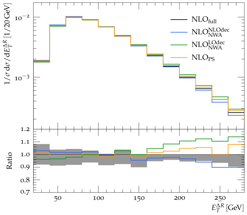
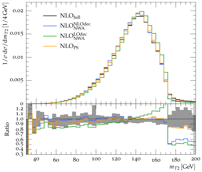
In Fig. 3, we show the normalised distribution of $m_{T2}$ as defined in Eq. (7), for the four theoretical descriptions. By construction, this observable has a sharp kinematic edge at $m_{T2}=m_{t}$, which is clearly visible and mildly washed out by off-shell effects, ambiguities related to missing energy and jet recombination. We find that for the $\mathrm{NLO_{full}}$ prediction, 97% of the total fiducial cross section is contained below $m_{T2}\leq m_{t}$. The shapes of the different theoretical descriptions follow patterns very similar to those observed for $m_{lb}$. In particular, the $\mathrm{NLO_{NWA}^{NLOdec}}$ prediction closely follows $\mathrm{NLO_{full}}$ up to the kinematic edge, with shape differences of a few percent, but in general within the scale uncertainty band.

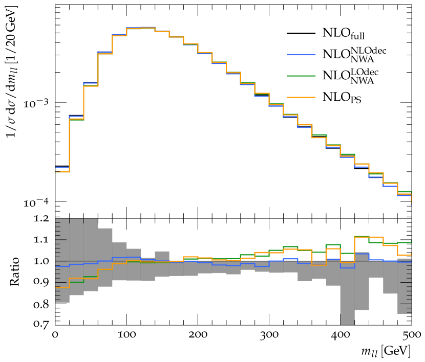
In Fig. 4(a), we show the di-lepton invariant mass $m_{ll}$. We observe that off-shell effects are small and that all theoretical descriptions agree at the 10% level. This is expected because $m_{ll}$ is an observable which is inclusive in what concerns extra radiation. The descriptions $\mathrm{NLO_{NWA}^{LOdec}}$ and $\mathrm{NLO_{PS}}$ show a very similar behaviour and are outside the uncertainty bands of the $\mathrm{NLO_{full}}$ prediction except for low $m_{ll}$ values. In Fig. 4(b), we display the $E_{T}^{\Delta R}$ observable defined in Eq. (8). Similar to $m_{ll}$, also for $E_{T}^{\Delta R}$, the $\mathrm{NLO_{full}}$ and $\mathrm{NLO_{NWA}^{NLOdec}}$ predictions do not exhibit large differences. However, the shapes of the $\mathrm{NLO_{NWA}^{LOdec}}$ and $\mathrm{NLO_{PS}}$ predictions differ considerably from the $\mathrm{NLO_{full}}$ prediction. In contrast to the $m_{ll}$ case, the $\mathrm{NLO_{NWA}^{LOdec}}$ and $\mathrm{NLO_{PS}}$ predictions also differ significantly from each other.

(a)

(b)

Figure 5: Normalised differential cross sections for (a) the rapidity of the muon, $\eta_{\mu}$, and (b) the transverse momentum of the muon, $p_{T,\mu}$. The ratios of different theoretical descriptions to $\mathrm{NLO_{full}}$ including its scale uncertainty band are also shown.

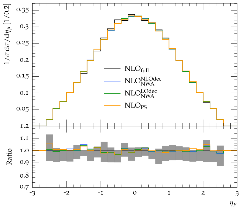
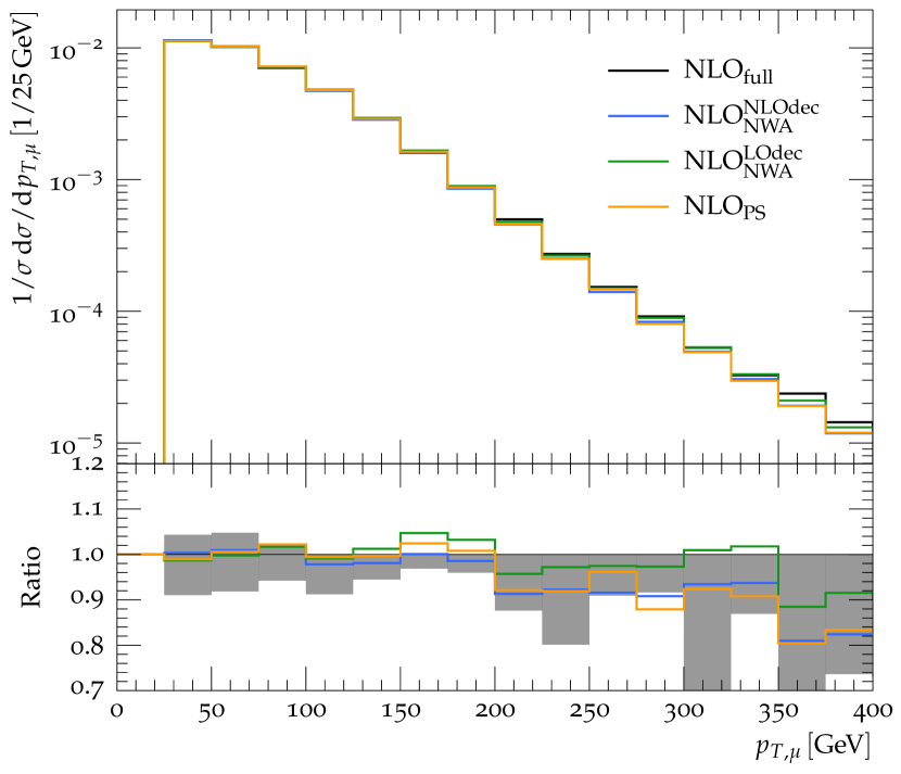
In Figs. 5(a) and 5(b), we show the muon rapidity $\eta_{\mu}$ and the muon transverse momentum $p_{T,\mu}$, respectively. Our four theoretical predictions for the $(e^{+}\nu_{e})\,(\mu^{-}\bar{\nu}_{\mu})\,b\bar{b}$ final state show a rather different behaviour in these two distributions. While the whole rapidity spectrum in Fig. 5(a) is properly modelled by all predictions, the transverse momentum spectrum in Fig. 5(b) is somewhat softer in the tail for the $\mathrm{NLO_{NWA}^{NLOdec}}$ and $\mathrm{NLO_{PS}}$ calculations with respect to $\mathrm{NLO_{full}}$. A possible interpretation is that non-resonant contributions in $\mathrm{NLO_{full}}$ contain $W$-bosons stemming from a hard collision rather than the top quark decay. Therefore they can carry higher energies which lead to a harder transverse momentum spectrum of the muon.

3.3.2 Scale dependence at LO and NLO

In this section, we will only consider the observables $m_{lb}$, $m_{T2}$, $m_{ll}$ and $E_{T}^{\Delta R}$, as they are promising with respect to at least one of the requirements of being observables with small systematics and/or high sensitivity to the top quark mass.

For $\mathrm{NLO_{full}}$, we compare LO and NLO predictions on the left-hand side, while in the figures on the right-hand side, we compare calculations based on the NWA, including scale variations. We observe that the NLO corrections in the $\mathrm{NLO_{full}}$ case lead to significant shape differences compared to $\mathrm{LO_{full}}$, see Figs. 6(a) to 9(a). While this is to be expected in the tails of the distributions, it is remarkable that the shape difference also affects the central and in particular the regions with low values of the observables. Given that the differences between the LO and NLO theory predictions in the full $W^{+}W^{-}b\bar{b}$ calculation are still sizeable in the bulk of the distributions, large differences in the top quark mass extracted from templates based on these predictions can be expected. The shape differences at low values of $m_{lb}$ and $m_{T2}$ are less pronounced in the calculations based on the NWA (with NLO in the $t\bar{t}$ production), as can be seen from Figs. 6(b) and 7(b). However, there are also significant shape differences in the bulk of the distribution. In addition, for the $m_{lb}$ distribution, Fig. 6(b), the peak is lower in the $\mathrm{NLO_{NWA}^{NLOdec}}$ and the $\mathrm{NLO_{PS}}$ case compared to the $\mathrm{NLO_{NWA}^{LOdec}}$ case, which can be easily understood considering the fact that more radiation, i.e. a harder distribution in the tail, softens the peak region.

(a)

(b)

Figure 6: Results including scale variation bands for $m_{lb}$, for (a) the $\mathrm{LO_{full}}$ and $\mathrm{NLO_{full}}$ calculations, (b) the calculations based on the NWA. The ratios with respect to (a) $\mathrm{LO_{full}}$ and (b) $\mathrm{NLO_{NWA}^{LOdec}}$ are also shown.

(a)

(b)

Figure 7: Results including scale variation bands for $m_{T2}$, for (a) the $\mathrm{LO_{full}}$ and $\mathrm{NLO_{full}}$ calculations, and (b) the calculations based on the NWA. The ratios are defined as in Fig. 6.

(a)

(b)

Figure 8: Results including scale variation bands for $m_{ll}$, for (a) the $\mathrm{LO_{full}}$ and $\mathrm{NLO_{full}}$ calculations, and (b) the calculations based on the NWA. The ratios are defined as in Fig. 6.

(a)

(b)

Figure 9: Results including scale variation bands for $E_{T}^{\Delta R}$ for (a) the $\mathrm{LO_{full}}$ and $\mathrm{NLO_{full}}$ calculations, and (b) the calculations based on the NWA. The ratios are defined as in Fig. 6.

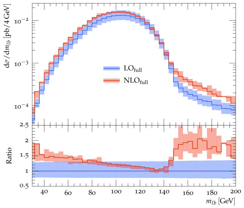
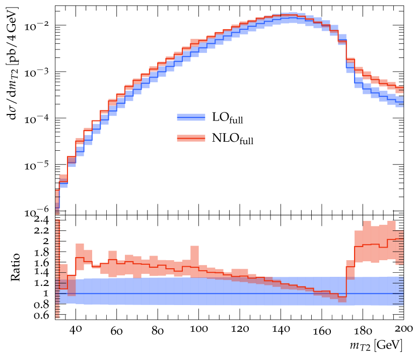
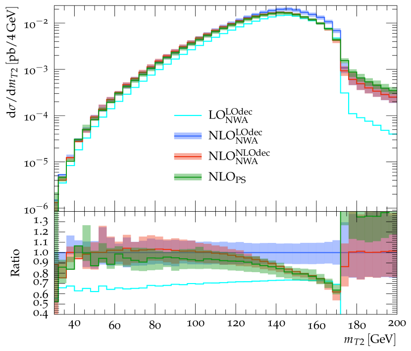
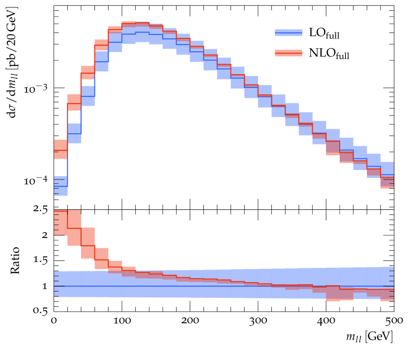
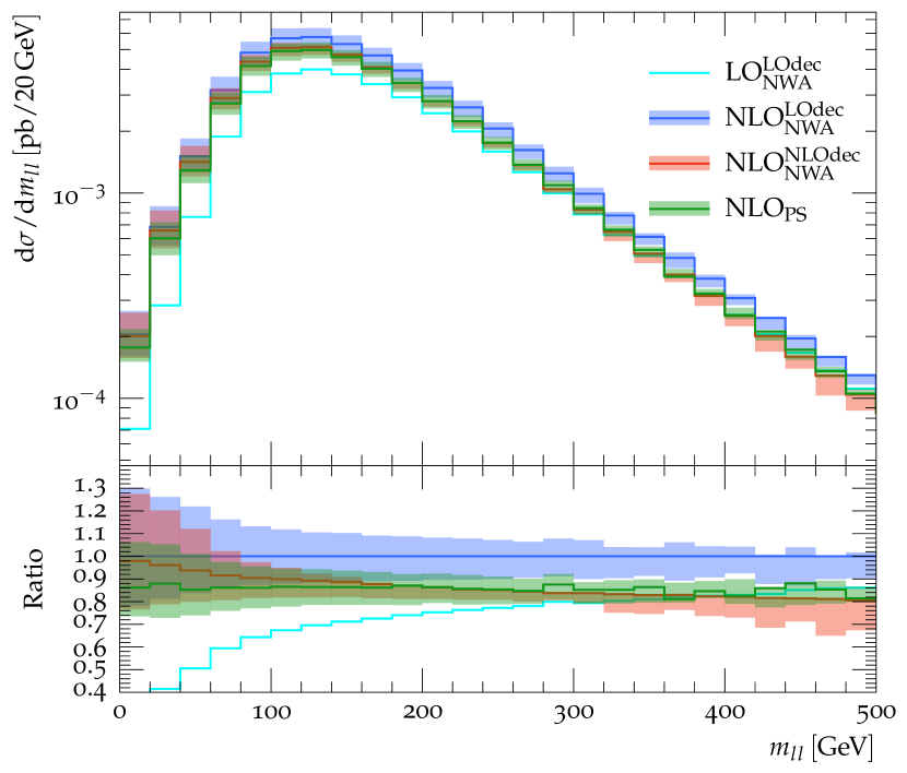
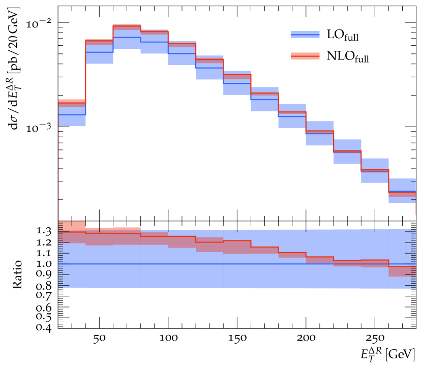
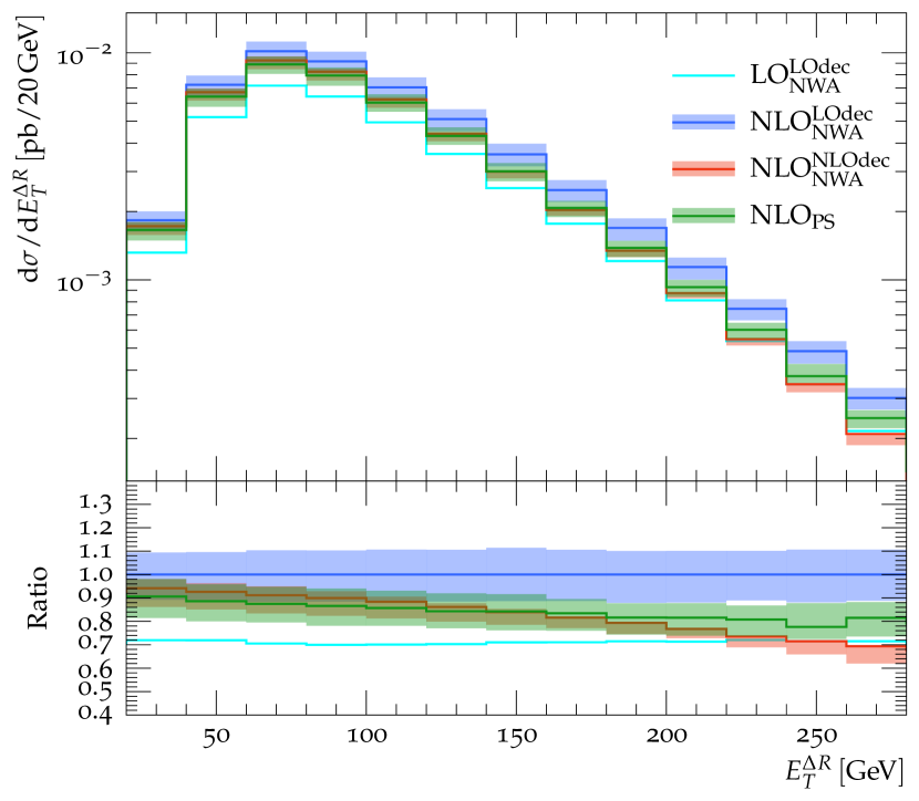
For the observable $m_{ll}$, the shape differences introduced by the $\mathrm{NLO_{full}}$ calculation at low $m_{ll}$ values are particularly pronounced in Fig. 8(a). The calculations based on the NWA in Fig. 8(b), $\mathrm{NLO_{NWA}^{NLOdec}}$ and $\mathrm{NLO_{NWA}^{LOdec}}$, cease to overlap at relatively low $m_{ll}$ values ($m_{ll}\sim 160\mathrm{\>GeV}$), while $\mathrm{NLO_{PS}}$ mostly lies between $\mathrm{NLO_{NWA}^{NLOdec}}$ and $\mathrm{NLO_{NWA}^{LOdec}}$ in the region beyond $m_{ll}>200\mathrm{\>GeV}$. As shown in Table 2, the total cross section predicted by $\mathrm{NLO_{PS}}$ is considerably smaller. This is due to the fact that after the shower, the $b$-jets are softer and therefore a larger fraction of events does not pass the requirement of two $b$-jets above $p_{T,\mathrm{min}}^{\mathrm{jet}}=25\mathrm{\>GeV}$. Even though the observable $m_{ll}$ does not involve jets, the jet requirements affect this observable, since we use the data set produced with the same requirements as for the other observables. A similar pattern is seen in the observable $E_{T}^{\Delta R}$ (Figs. 9(a) and 9(b)).

The scale variation bands in the $\mathrm{NLO_{full}}$ case and the $\mathrm{NLO_{NWA}^{NLOdec}}$ case are rather asymmetric: the central scale leads to the largest differential cross section compared to up- and downwards variations over a large kinematic range of the corresponding observable. This effect is particularly pronounced for the $m_{ll}$ and $E_{T}^{\Delta R}$ distributions.

3.3.3 Distributions for several top quark masses

(a)

(b)

Figure 10: Effect of top quark mass variations on the normalised differential cross sections for $m_{lb}$ and $m_{T2}$. We also show the ratios to the prediction obtained with $m_{t}=172.5\mathrm{\>GeV}$. All results are obtained with the $\mathrm{NLO_{full}}$ description for the $13\mathrm{\>TeV}$ LHC.

(a)

(b)

Figure 11: Effect of top quark mass variation on the normalised differential cross section for $m_{ll}$ and $E_{T}^{\Delta R}$. We also show the ratios to the prediction obtained with $m_{t}=172.5\mathrm{\>GeV}$. The results are obtained with the $\mathrm{NLO_{full}}$ description for the $13\mathrm{\>TeV}$ LHC.

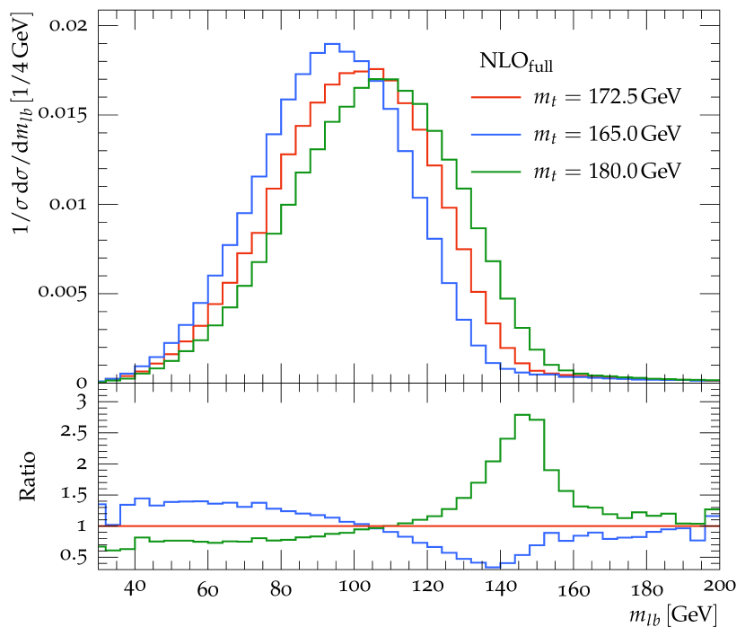
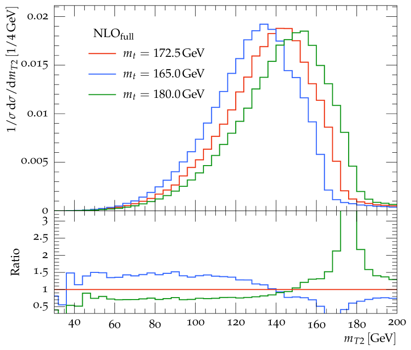
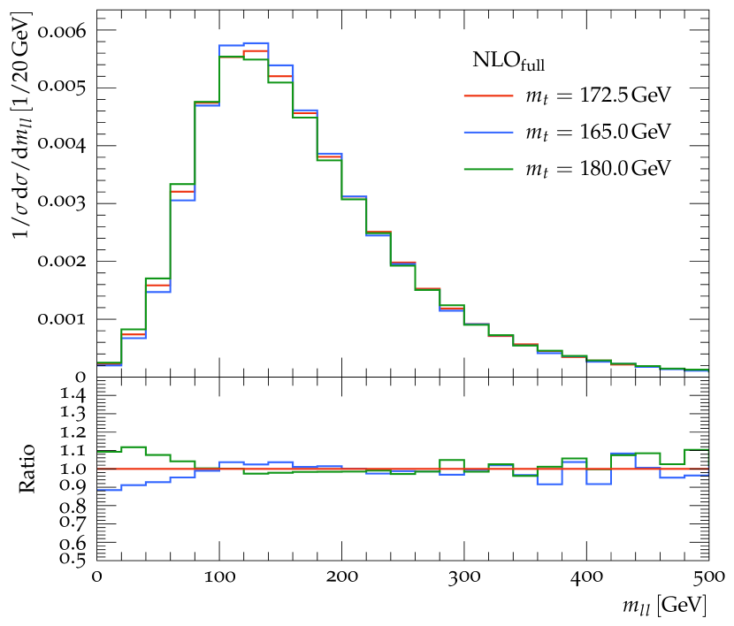
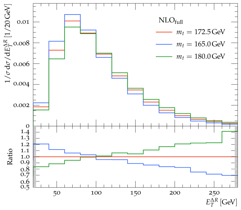
In this section, we investigate the sensitivity of the four observables $m_{lb}$, $m_{T2}$, $m_{ll}$ and $E_{T}^{\Delta R}$ to variations of the top quark mass. We exploit distributions based on the $\mathrm{NLO_{full}}$ calculation using the three values, $m_{t}=165$, $172.5$, $180\mathrm{\>GeV}$, for the top quark mass.

We observe a strong sensitivity of the $m_{lb}$ and $m_{T2}$ distributions to the top quark mass with ratios up to about three in the given range. A lower top quark mass naturally leads to a softer spectrum while a higher top quark mass leads to a harder spectrum in these two observables. The sensitivity of $m_{ll}$ is shown in Fig. 11(a) and turns out to be very small. Unfortunately, being a purely leptonic observable, the low sensitivity counterbalances its expected Frixione:2014ala better experimental systematics. Compared to the $m_{ll}$ distribution, the $E_{T}^{\Delta R}$ distribution in Fig. 11(b) shows a somewhat larger sensitivity to $m_{t}$, albeit much smaller than what is observed for $m_{lb}$ and $m_{T2}$.

4 Measurement of the top quark mass based on pseudo-data

The top quark mass measurements in the di-lepton channel presented in Refs. Aad:2015nba ; AMaierPhD:2015 ; Aaboud:2016igd use the template method. In this method, simulated distributions are constructed for different input values of the top quark mass, $m^{\mathrm{in}}_{t}$. The distributions (templates) per $m^{\mathrm{in}}_{t}$ are then individually fitted to a suitable function. Using templates at different $m^{\mathrm{in}}_{t}$, it is verified that all parameters of the function linearly depend on $m_{t}=m^{\mathrm{in}}_{t}$. Consequently, this linearity is imposed in a combined fit to all templates. This fit fixes the theory prediction (i.e. the parametrisation of the theory hypothesis) by determining all parameters of the function, except for $m_{t}$ and the absolute normalisation. The former is to be determined from the data and represents the fit result, while the latter is left as a free parameter. We therefore follow the experimental procedure to neglect the absolute normalisation in the fit to avoid a dependence on the involved experimental determination of the total luminosity and detector efficiency. This choice makes the results of this study independent of the total cross section of the respective calculations, leaving shape changes of the differential distributions as the measure for $m_{t}$. Using those parameter values, a likelihood fit of this function to data is performed to obtain the value for $m_{t}$ that best describes the data, namely $m^{\mathrm{out}}_{t}$, together with its statistical uncertainty.

In experimental analyses, these templates are constructed at the detector level, i.e. mimicking real data. Here, an analogous procedure is employed to assess the impact of different theory descriptions on the template method used to determine the top quark mass. In our analysis, the pseudo-data mimicking experimental data (i.e. the data model) in each figure are always generated from those predictions, which are believed to be closer to real data, i.e. those that are considered to give the “better” result. We simulate a data luminosity of $50/\mathrm{fb}$.

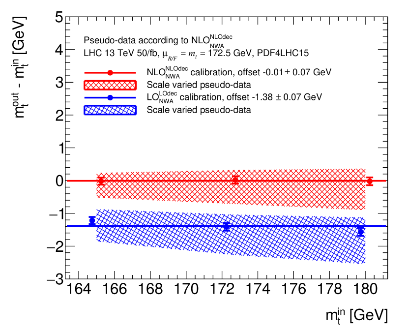
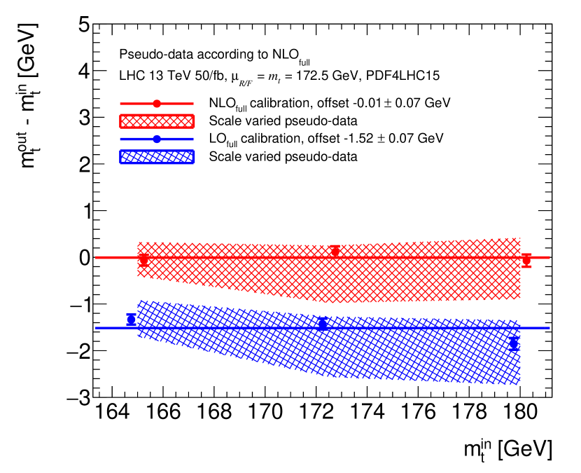
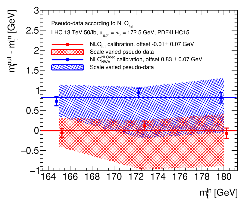
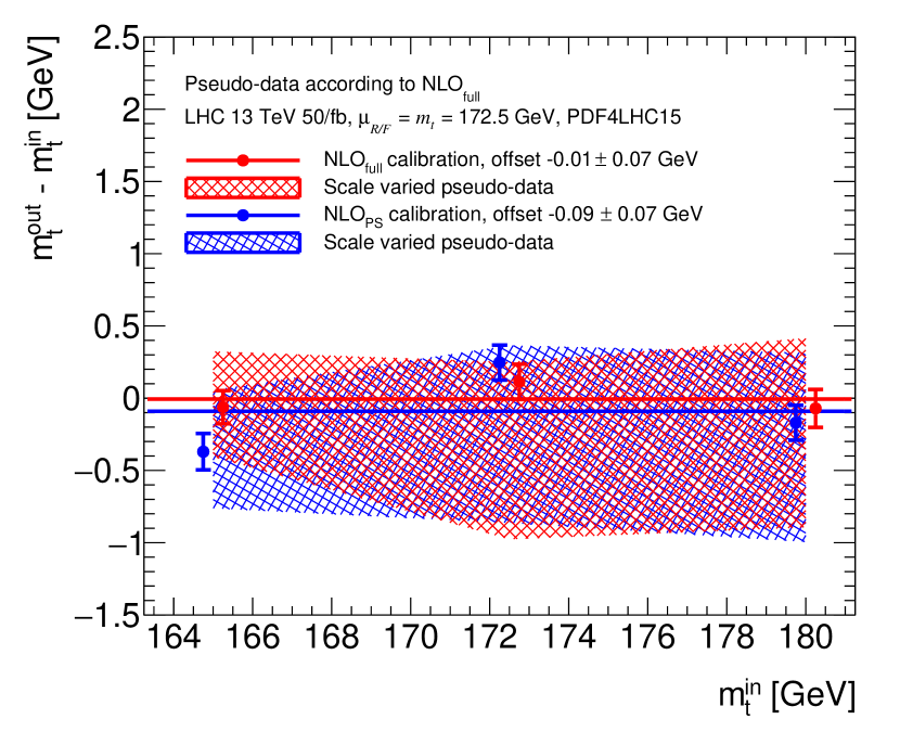
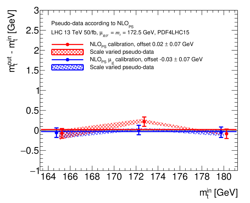
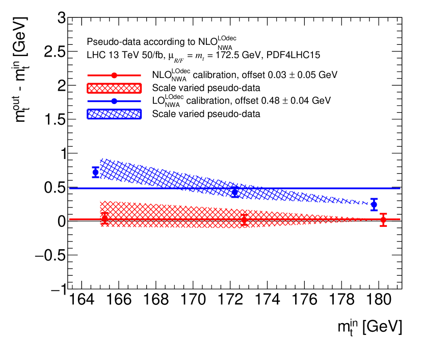
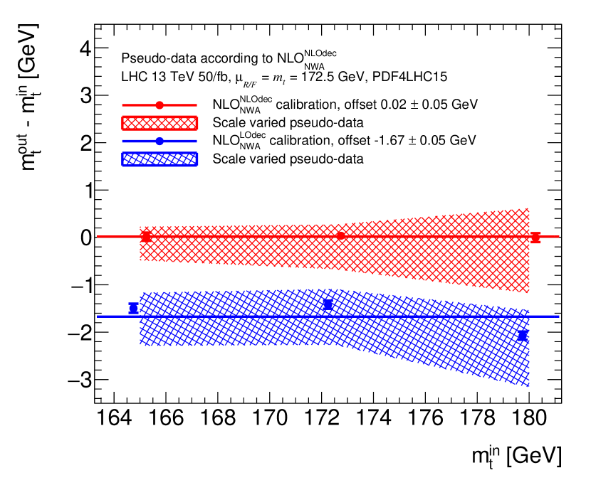
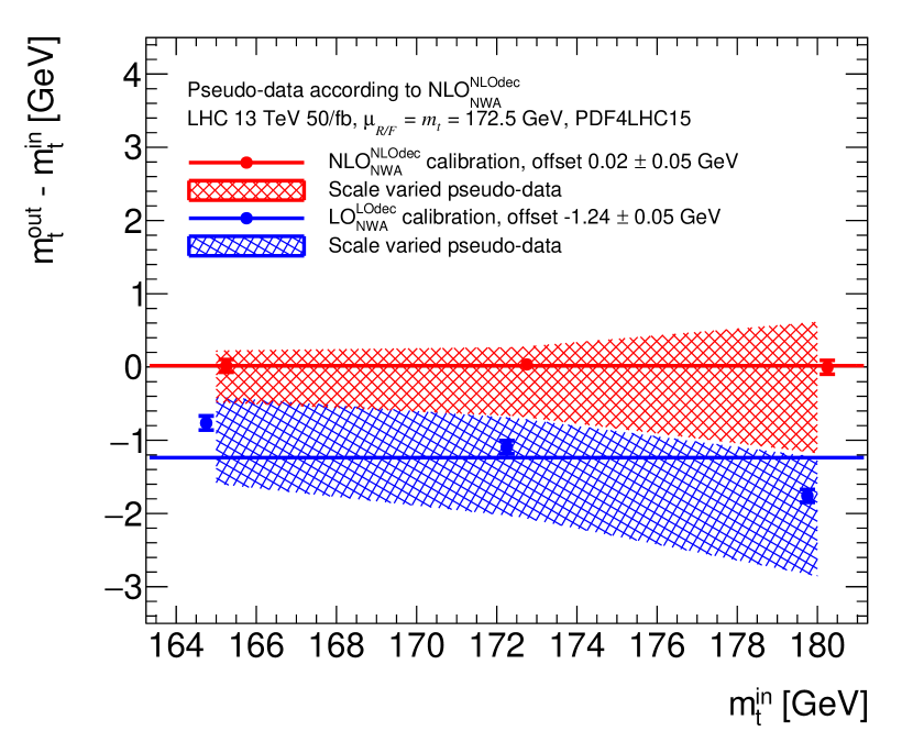
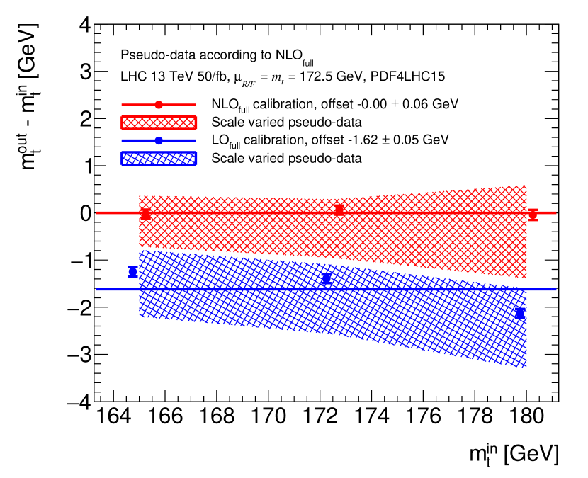
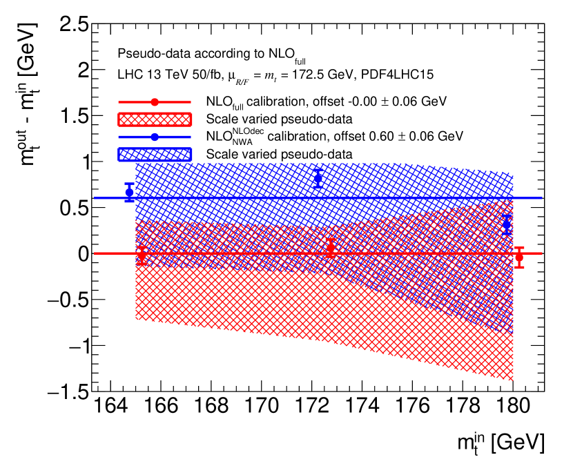
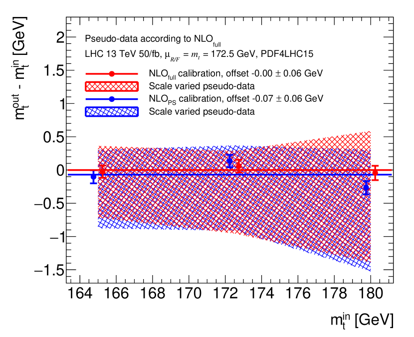
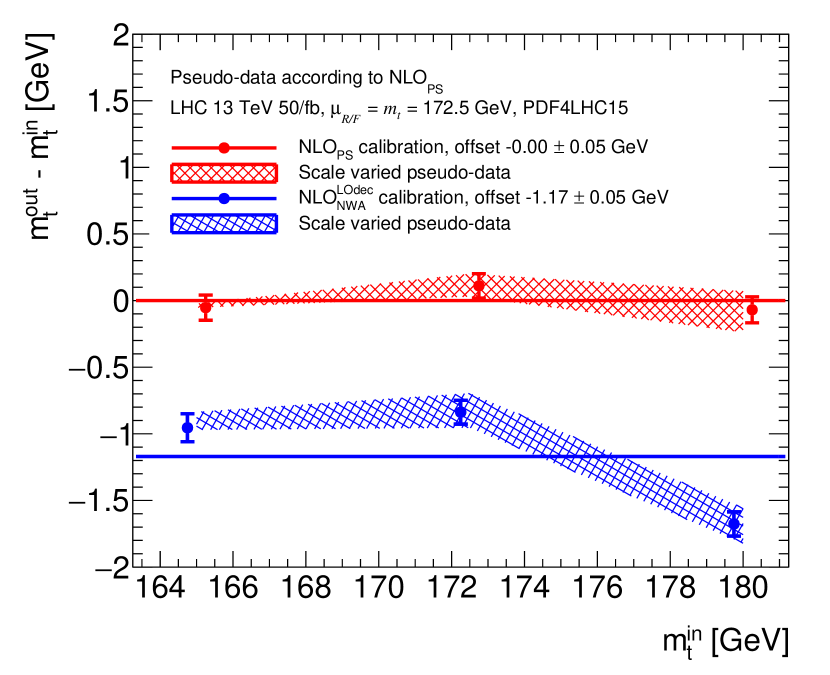
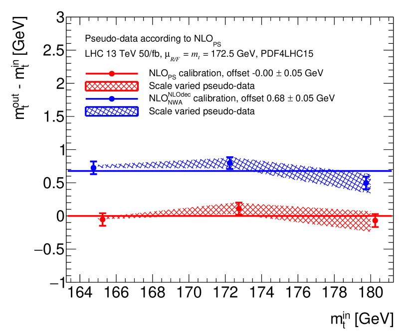
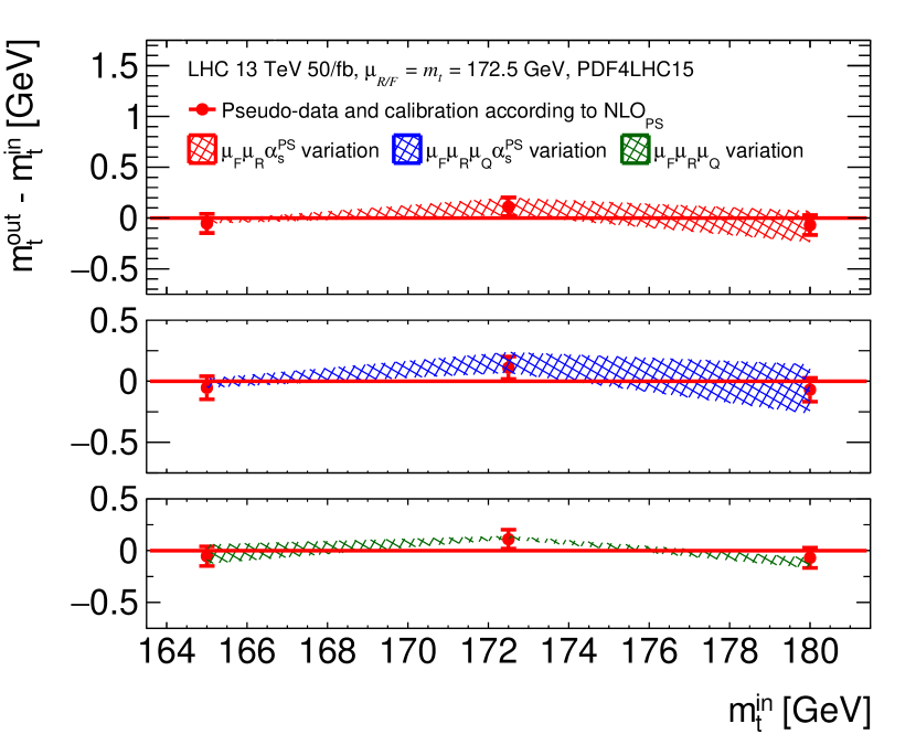
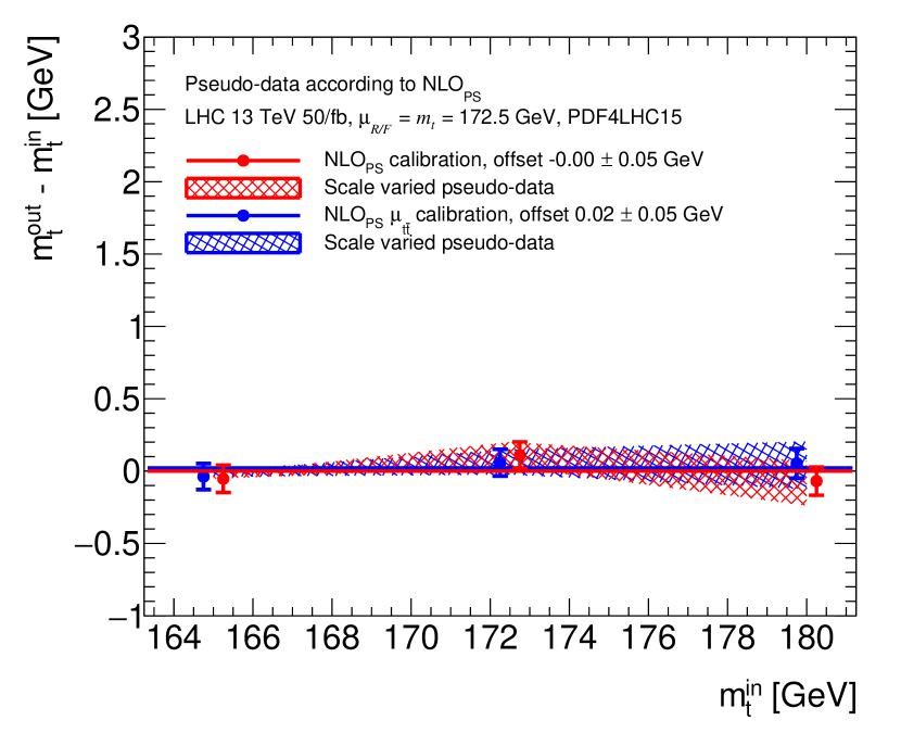
The sensitivity to the theoretical assumptions and their uncertainties is assessed by fits to one thousand pseudo-data sets created by random sampling from the underlying theory prediction. The layout of Figure 12(a) is representative for an entire set of figures presented in the following. For three different values of $m^{\mathrm{in}}_{t}$, each of these figures shows the observed difference of $m^{\mathrm{out}}_{t}$, the mass measured by the procedure, and $m^{\mathrm{in}}_{t}$, the mass used to generate the pseudo-data. The red/blue points correspond to the mean difference observed for all pseudo-data sets that are produced as stated in the second line of the figure legends, and analysed with the template fit functions (the theory hypothesis), denoted by “calibration” in the legend for the red/blue points. The uncertainty per point is statistical only and corresponds to the expected experimental uncertainty for the assumed data luminosity. The points are displaced on the horizontal axis to ensure better visibility in the case of overlapping bands. The horizontal lines stem from a fit of the three points to a constant, displaying the average offset. The values given are the (individual) offsets together with their statistical uncertainties. The bands indicate the effect of the scale variations on the measured $m_{t}$. They are obtained by replacing the central-scale pseudo-data by those derived from the associated samples, which were calculated using the varied scales.

The ranges of the fits have been chosen on a plateau of good fit performance and high mass sensitivity. The ranges of choice are

$$40\mathrm{\>GeV}\leq m_{lb}\leq 160\mathrm{\>GeV}\;,$$ (16)

$$80\mathrm{\>GeV}\leq m_{T2}\leq 180\mathrm{\>GeV}\;.$$

Note that for the $\mathrm{NLO_{PS}}$ calculations employing the $\mu_{t\bar{t}}$ scale, we used a fit range of $50\mathrm{\>GeV}\leq m_{lb}\leq 150\mathrm{\>GeV}$.

As the range around the kinematic edge is a particularly $m_{t}$-sensitive region, the question arises how much our results depend on the chosen fit range. Therefore we produced another set of fits where we restricted the fit range to $m_{lb}<140\mathrm{\>GeV}$, and found that the results are sufficiently stable under this change of the fit range. The results of both fit ranges are reported below.

4.1 Fit results for $m_{lb}$

(a)

(b)

Figure 12: Results of the top quark mass determination using the observable $m_{lb}$ and (a) pseudo-data generated according to the factorised approach with $\mathrm{NLO_{NWA}^{LOdec}}$, showing the effect of changing the perturbative order in the production process only, and (b) pseudo-data obtained from the factorised approach with $\mathrm{NLO_{NWA}^{NLOdec}}$, showing the effect of changing the perturbative order in the decay process only.

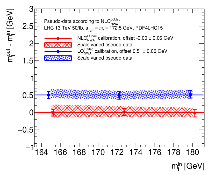
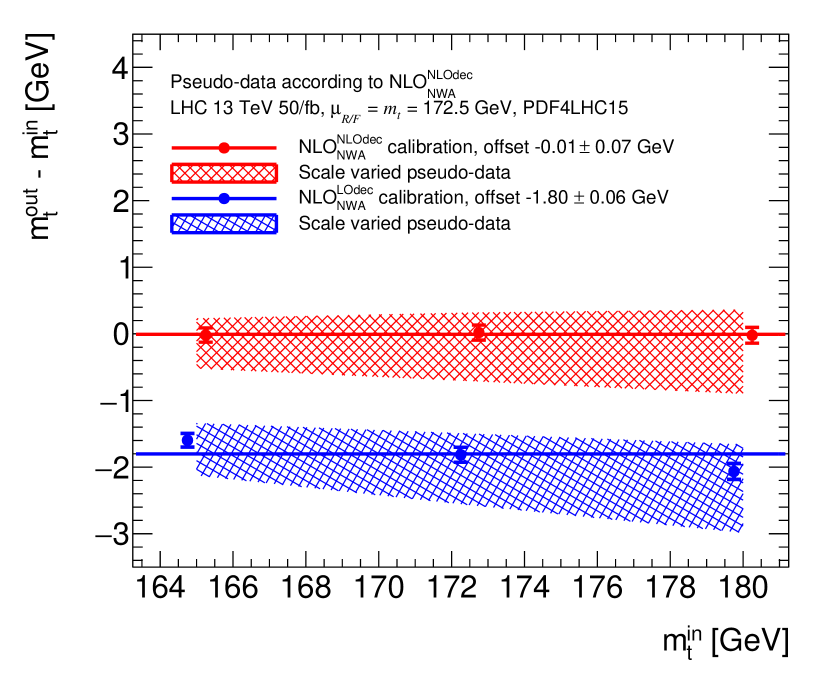
Figure 12(a) shows results of a fit where the pseudo-data have been generated using the factorised approach with $\mathrm{NLO_{NWA}^{LOdec}}$. The fit has been performed once with $\mathrm{LO_{NWA}^{LOdec}}$ as the theory model (blue) and once with $\mathrm{NLO_{NWA}^{LOdec}}$ (red). The vanishing offset (i.e. it is compatible with zero) for the red lines (here and in all the following figures) proves that the method is closed, i.e. it finds the input value when the pseudo-data and the calibration coincide. The offset between the blue and red lines in Fig. 12(a) shows the effect of changing the perturbative order of the production process in the theory model. The offset of $0.51\pm 0.06\,\mathrm{\>GeV}$ demonstrates that these corrections have an impact on the mass determination at the level of the present experimental uncertainties. As the fits are based on normalised differential cross sections, the bands are sensitive to shape differences induced by the scale variations, rather than to their overall magnitudes.

Figure 12(b) shows results of a fit where the pseudo-data have been generated using the factorised approach based on the $\mathrm{NLO_{NWA}^{NLOdec}}$, i.e. the NWA at NLO, while the theory models differ in the decay order only. We observe that the effect of an ${\cal O}({\alpha_{s}})$ change in the perturbative order of the decay is more significant than changing the order in the production process. The offset stemming from the former amounts to $-1.80\pm 0.06\mathrm{\>GeV}$, while switching from LO to NLO in the description of the production process yields an offset of $0.51\pm 0.06\mathrm{\>GeV}$ (cf. Fig. 12(a)). In addition, the size of the uncertainty bands increases because the NLO corrections to the decay lead to non-uniform scale variation bands.

Figure 13(a) shows the effect of changing the perturbative order in both the production and decay process. Comparing Figs. 12 and 13(a), we observe that, within the statistical uncertainties, the offset in Fig. 13(a) coincides with the sum of the offsets in Figs. 12(a) and 12(b), as is expected for the factorised approach. Figure 13(b) shows results of a fit where the pseudo-data have been generated using the $\mathrm{NLO_{full}}$ calculation, and the calibrations are based on the $\mathrm{NLO_{full}}$ and $\mathrm{LO_{full}}$ descriptions. While the uncertainty bands are comparable to the factorised case that uses pseudo-data based on $\mathrm{NLO_{NWA}^{NLOdec}}$ (Fig. 13(a)), the offset increases from $-1.38\pm 0.07\mathrm{\>GeV}$ to $-1.52\pm 0.07\mathrm{\>GeV}$. While this increase in the offset is not conclusive when taking the statistical uncertainty into account, it still is an indication of the trend that the inclusion of a richer set of corrections leads to larger offsets.

(a)

(b)

Figure 13: Results of the top quark mass determination using the observable $m_{lb}$ and (a) pseudo-data generated according to the factorised approach with $\mathrm{NLO_{NWA}^{NLOdec}}$, showing the effect of changing the perturbative order in both the production and decay process, and (b) pseudo-data derived from $\mathrm{NLO_{full}}$ distributions. In both cases, the focus is on the comparison of LO versus NLO calibrations.

In Fig. 14(a), we again use pseudo-data generated according to $\mathrm{NLO_{full}}$, this time comparing the fit based on the full NLO calibration to the one obtained with the $\mathrm{NLO_{NWA}^{NLOdec}}$ calibration representing the factorised NLO approach. We see that the offset of $0.83\pm 0.07\mathrm{\>GeV}$ is smaller in magnitude than in Fig. 13(b), and goes in the opposite direction. This indicates that the non-factorisable contributions are suppressed in the fit range, since the NWA, with the corrections to the decay included, is a better approximation than $\mathrm{LO_{full}}$ only.

In Fig. 14(b), we replace the $\mathrm{NLO_{NWA}^{NLOdec}}$ calibration by the one from the $\mathrm{NLO_{PS}}$ prediction. We observe an offset of $-0.09\pm 0.07\mathrm{\>GeV}$, which is surprisingly small compared to that given in Fig. 14(a). It is expected that the two NWA-based descriptions, both including the leading radiation in the decay, lead to quite similar results. However, the $\mathrm{NLO_{PS}}$ simulation differs from the $\mathrm{NLO_{NWA}^{NLOdec}}$ calculation in a number of points. While $\mathrm{NLO_{PS}}$ falls short of describing the top quark decay beyond the soft limit owing to the absence of decay matrix-element corrections, the parton shower approach generates a very different, more complete QCD radiation pattern as a result of including resummation effects in the production as well as the decay of the top quarks. This means that the two stages of $t\bar{t}$ production and decay are not factorised in exactly the same way as in the $\mathrm{NLO_{NWA}^{NLOdec}}$ calculation. These differences explain why the offset in Fig. 14(a) is different from the one in Fig. 14(b). In fact, as can be seen from Figs. 2 as well as 6(b), the emission pattern and resummation effects of the $\mathrm{NLO_{PS}}$ case are relevant at lower $m_{lb}$ values and in particular around (and above) the kinematic edge, and lead to a shape of the $m_{lb}$ distribution, which differs from the fixed-order $\mathrm{NLO_{NWA}^{NLOdec}}$ case. Especially for the $m_{lb}\sim 140\mathrm{\>GeV}$ region, we notice that the agreement between $\mathrm{NLO_{PS}}$ and $\mathrm{NLO_{full}}$ is better than between $\mathrm{NLO_{PS}}$ and $\mathrm{NLO_{NWA}^{NLOdec}}$. This is an indication that in this region, resummation effects are more important than the inclusion of the radiative correction in the decay. The nearly vanishing mass offset shown in Fig. 14(b) occurs due to the fact that the shapes of $\mathrm{NLO_{PS}}$ and $\mathrm{NLO_{full}}$ do not differ significantly in most of the fit range, despite their different theoretical content.

(a)

(b)

Figure 14: Top quark mass determination results for the observable $m_{lb}$ comparing pseudo-data generated according to the $\mathrm{NLO_{full}}$ predictions with (a) the $\mathrm{NLO_{NWA}^{NLOdec}}$ calibration and (b) the $\mathrm{NLO_{PS}}$ calibration.

In Fig. 15, we use pseudo-data generated according to the $\mathrm{NLO_{PS}}$ prediction using the scale setting $\mu_{F}=\mu_{R}=m_{t}$. The related scale variations have been obtained by employing the $\mu_{F}\mu_{R}{\alpha^{\mathrm{PS}}_{s}}$ scheme as described at the end of Section 3.2. By comparing to Fig. 12(a), we observe that the uncertainty bands of $\mathrm{NLO_{PS}}$ are smaller than the ones for $\mathrm{NLO_{NWA}^{LOdec}}$. However, for the theory models relying on NLO decays, as shown in Fig. 12(b) for $\mathrm{NLO_{NWA}^{NLOdec}}$ and in Fig. 13(b) for $\mathrm{NLO_{full}}$, the bands are much wider. Hence, we expect that adding a parton shower to the $\mathrm{NLO_{full}}$ calculation, the bands would persist or be only slightly reduced, analogous to the LO decay situation discussed above.

Unlike the case presented in Fig. 14(b), the direct comparison between results from the NWAs and $\mathrm{NLO_{PS}}$ produces non-vanishing mass shifts. If we analyse the $\mathrm{NLO_{PS}}$ pseudo-data using the fixed-order $\mathrm{NLO_{NWA}^{LOdec}}$ calibration, we find a mass offset of $-0.92\pm 0.07\mathrm{\>GeV}$ as shown in Fig. 15(a). This indicates that the parton shower emissions (in both stages), supplementing the NLO accurate $t\bar{t}$ production, have a considerable impact on the results. In addition, a significant dependence of the $\mathrm{NLO_{NWA}^{LOdec}}$ calibration offset on the top quark mass is observed, i.e. the blue points are inconsistent with the constant fit. This implies that the $\mathrm{NLO_{NWA}^{LOdec}}$ $m_{lb}$ distribution has a stronger dependence on the top quark mass than the one generated by $\mathrm{NLO_{PS}}$. A similar trend has been seen in Fig. 12(b), where $\mathrm{NLO_{NWA}^{LOdec}}$ is compared to $\mathrm{NLO_{NWA}^{NLOdec}}$. Turning to Fig. 15(b), we show the case where the $\mathrm{NLO_{PS}}$ pseudo-data have been confronted with the improved fixed-order model $\mathrm{NLO_{NWA}^{NLOdec}}$. For this case, we would expect a pseudo-data-theory agreement which is better than the one seen in Fig. 15(a), since both the $\mathrm{NLO_{PS}}$ and the $\mathrm{NLO_{NWA}^{NLOdec}}$ description contain the major contributions to describe the extra emission in the top quark decays. However, the offset of $0.96\pm 0.07\mathrm{\>GeV}$ is similar in size (while opposite in direction) compared to the LO decay case shown in Fig. 15(a). This is consistent with the offset differences shown in Table 3, for example subtracting the offset given in Fig. 12(b) from the one in Fig. 15(a), or alternatively the one in Fig. 14(b) from the one in Fig. 14(a).

(a)

(b)

Figure 15: Top quark mass determination results for the observable $m_{lb}$ comparing pseudo-data generated according to the $\mathrm{NLO_{PS}}$ predictions with (a) the $\mathrm{NLO_{NWA}^{LOdec}}$ calibration and (b) the $\mathrm{NLO_{NWA}^{NLOdec}}$ calibration.

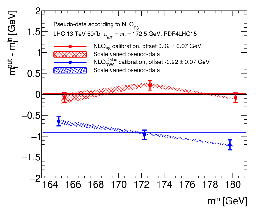
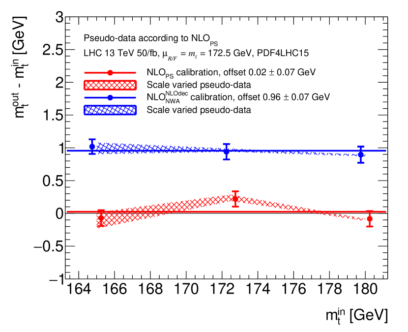
Further investigations are needed to understand the source of the mass shift observed in Fig. 15(b). Based on the current findings, we cannot conclude whether it originates from ($i$) the inclusion of resummation effects, or ($ii$) genuine differences in incorporating the fixed-order QCD corrections to the production and decay of the top quark pairs, or both. The different radiation patterns generated by $\mathrm{NLO_{PS}}$ and $\mathrm{NLO_{NWA}^{NLOdec}}$ do not allow for a strict, same-level comparison between the two approaches, but reducing the amount of radiation produced by $\mathrm{NLO_{PS}}$ is expected to bring them closer to each other, and to diminish the role of resummation effects.

There is no unique way of limiting the scope of the resummation. To control the generation of a reduced branching pattern, we use an approach where each showering process can be terminated after a (given) fixed number of emissions, denoted by $n_{\mathrm{max}}$. For our study, we rely on the fully factorised version of combining the subshowers, i.e. we separately restrict the number of emissions to no more than $n$ ($n_{\mathrm{max}}^{\mathrm{prod}}=n_{\mathrm{max}}^{\mathrm{dec}}=n$) in each subshower (the primary one evolving the $t\bar{t}$ production and the secondary one evolving the decays). The combination of one-emission production and decay showers ($n_{\mathrm{max}}^{\mathrm{prod}}=n_{\mathrm{max}}^{\mathrm{dec}}=1$) can then be used to emulate the $\mathrm{NLO_{NWA}^{NLOdec}}$ calculation, which enables us to approximately separate effects ($i$) from ($ii$). In addition, comparing the restricted and full $\mathrm{NLO_{PS}}$ prescriptions will provide us with a qualitative estimate of the impact of the full resummation. Starting from $n_{\mathrm{max}}^{\mathrm{prod}}=1$ and $n_{\mathrm{max}}^{\mathrm{dec}}=1$, we can successively restore the full shower by incrementing the number of emissions.

(a)

(b)

Figure 16: Results of the restricted-shower study for the $m_{lb}$ observable using $\mathrm{NLO}_{\mathrm{PS}}^{(n_{\mathrm{max}}^{\mathrm{prod}},n_{\mathrm{max}}^{\mathrm{dec}})}$ parton showers that terminate after a certain maximal number of emissions in both the production and decay showers. In (a) mass offsets are shown for a number of pseudo-data sets using the $\mathrm{NLO_{NWA}^{NLOdec}}$ and the $\mathrm{NLO_{PS}}$ calibrations in the shape analysis. The sets of pseudo-data are generated according to the $\mathrm{NLO_{NWA}^{NLOdec}}$ description, the default $\mathrm{NLO_{PS}}$ as well as three $\mathrm{NLO_{PS}}$ showers that differ in $n_{\mathrm{max}}^{\mathrm{prod}}=n_{\mathrm{max}}^{\mathrm{dec}}=n_{\mathrm{max}}$. The corresponding $m_{lb}$ distributions for the case $m_{t}=172.5\mathrm{\>GeV}$ are given in (b).

(a)

(b)

Figure 17: Results of the restricted-shower study for the $m_{lb}$ observable using pure production, pure decay and pure LO parton showers only. In (a) mass offsets are shown for a number of pseudo-data sets using the $\mathrm{NLO_{NWA}^{NLOdec}}$ and the $\mathrm{NLO_{PS}}$ calibrations in the shape analysis. The sets of pseudo-data are generated according to the $\mathrm{NLO_{NWA}^{NLOdec}}$ description, the default $\mathrm{NLO_{PS}}$ and $\mathrm{LO_{PS}}$ showers as well as $\mathrm{NLO_{PS}}$ showers whose evolution is restricted to the production or decay stage only. The corresponding $m_{lb}$ distributions for the case $m_{t}=172.5\mathrm{\>GeV}$ are given in (b).

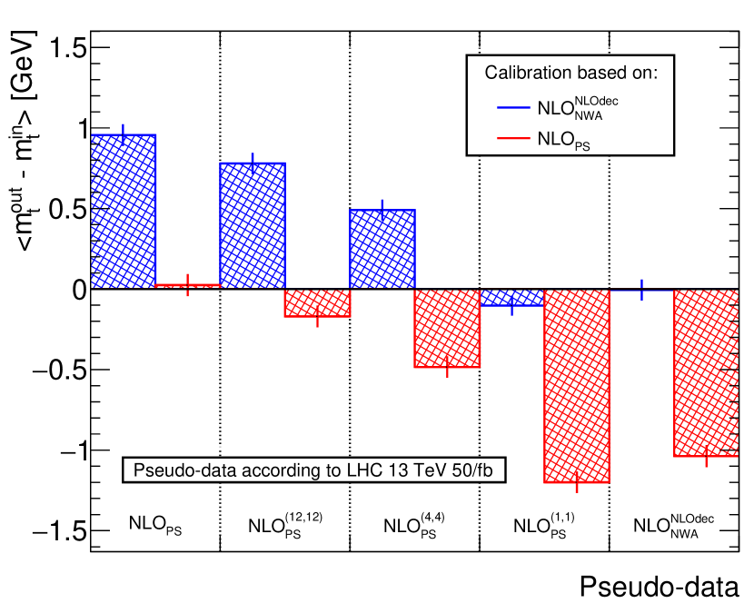
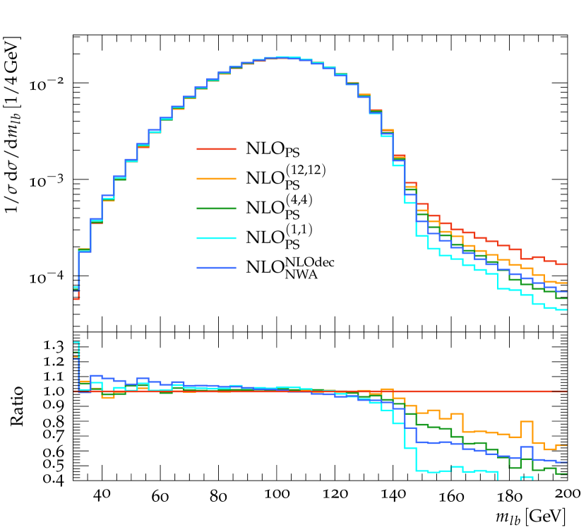
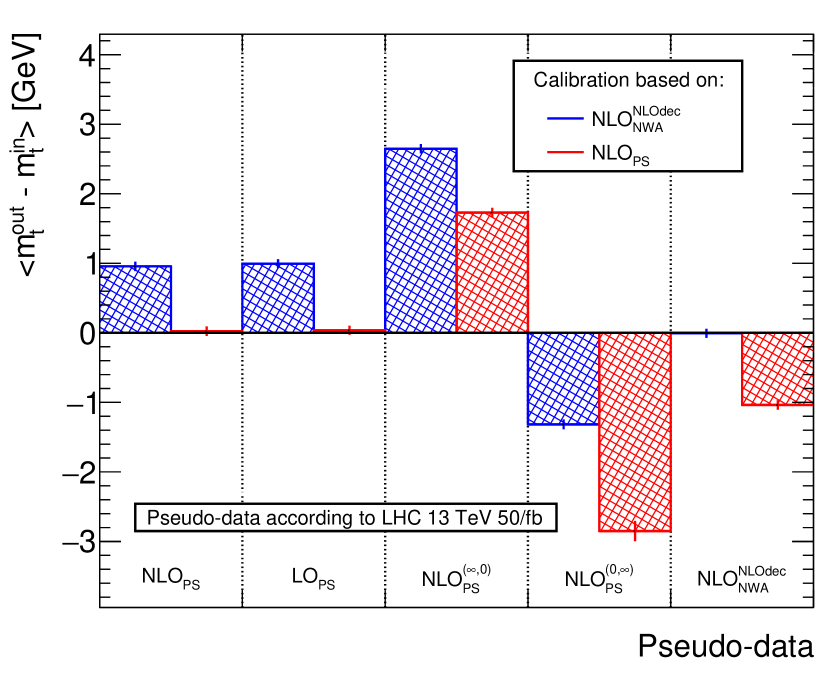
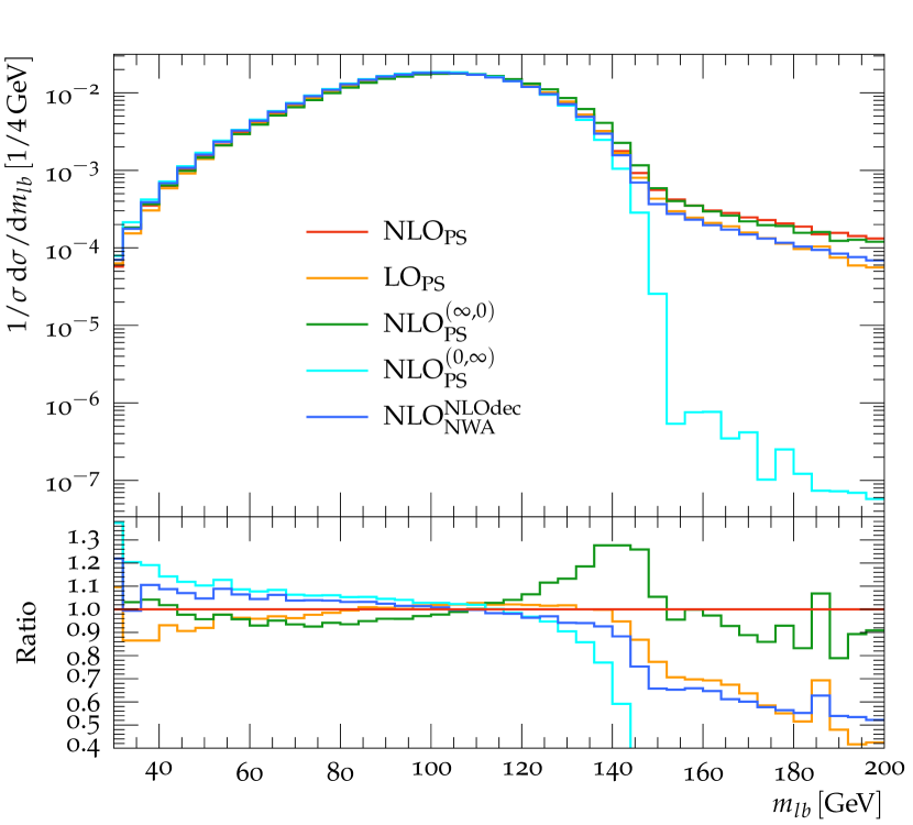
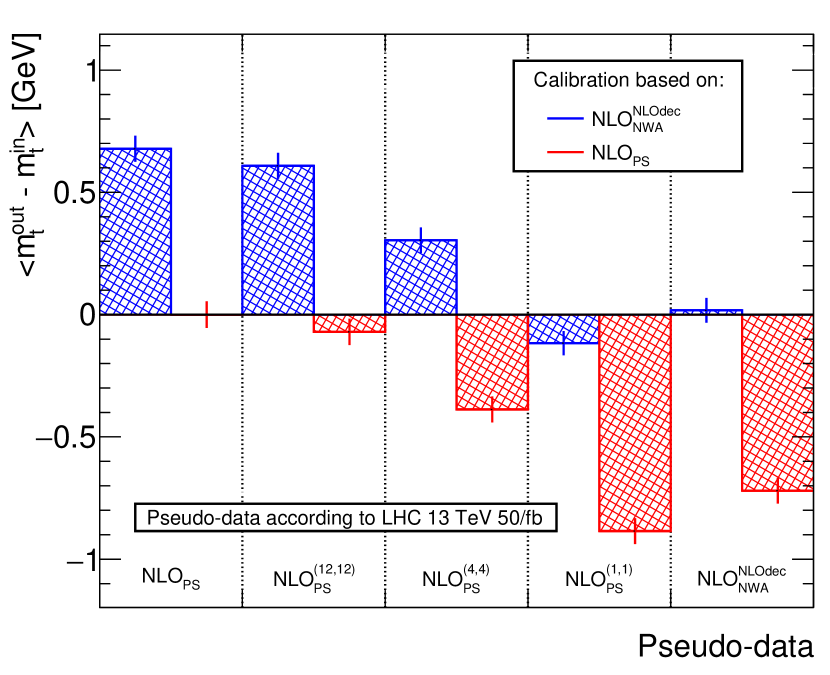
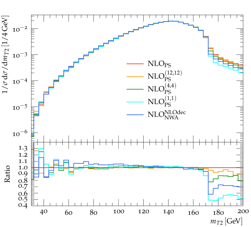
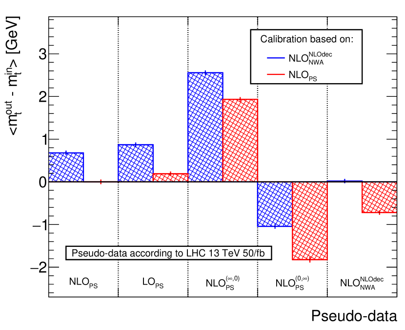
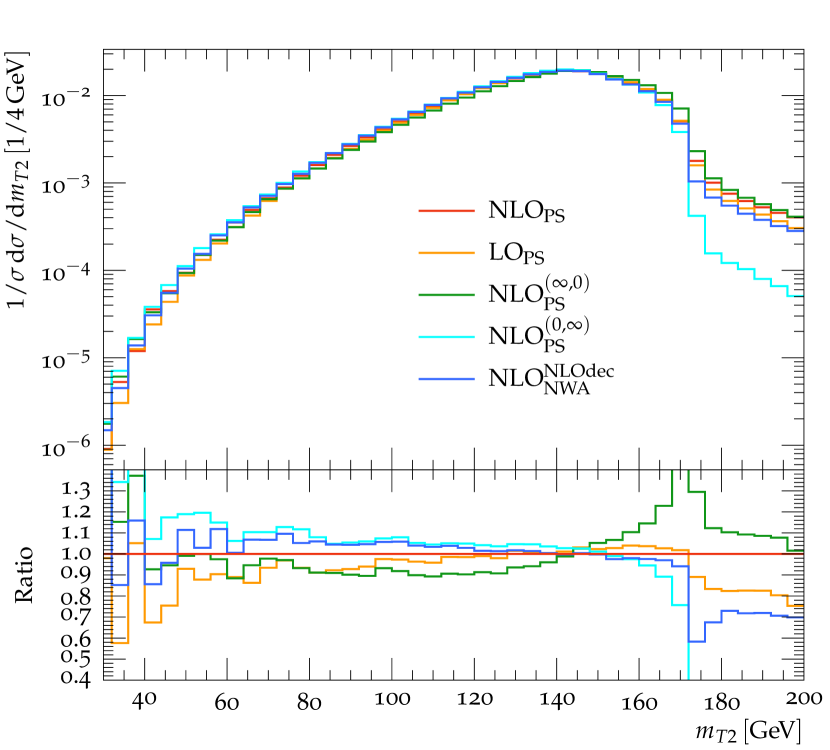
Figure 16 summarises the results of the restricted-shower studies. Figure 16(a) shows the offsets and their statistical uncertainties for sets of pseudo-data analysed with two calibrations, namely $\mathrm{NLO_{PS}}$ and $\mathrm{NLO_{NWA}^{NLOdec}}$, while the figure to the right, Fig. 16(b), depicts the corresponding $m_{lb}$ distributions. The leftmost bin in Fig. 16(a) corresponds to the mass shifts displayed in Fig. 15(b). The blue bar depicts the offset of the $\mathrm{NLO_{PS}}$ pseudo-data, analysed with the $\mathrm{NLO_{NWA}^{NLOdec}}$ calibration. The almost vanishing red bar shows the closure for the $\mathrm{NLO_{PS}}$ pseudo-data and calibration. Moving to the right, the parton shower is more and more restricted, allowing for at most $12$, $4$ and $1$ emissions in each subshower. This results in a smooth transition from the offset of $0.96\pm 0.07\mathrm{\>GeV}$ to almost zero (with an indication of a small overshoot to negative offsets). The mass shifts becoming fairly small for more restricted showering indicate that most of the differences between the $\mathrm{NLO_{NWA}^{NLOdec}}$ and $\mathrm{NLO_{PS}}$ predictions emerge from resummation effects. Finally, the rightmost bin is for the $\mathrm{NLO_{NWA}^{NLOdec}}$ pseudo-data themselves.

The calculated offsets, obtained from fits to the $m_{lb}$ distributions like the ones in Fig. 16(b), receive contributions from regions with large differential cross sections and small differences between restricted shower and calibration ($\mathrm{NLO_{NWA}^{NLOdec}}$ and $\mathrm{NLO_{PS}}$) results, as well as from regions with small differential cross sections and relatively large differences. The interplay of these effects can lead to situations such as the one observed here, where the mass offsets obtained from $\mathrm{NLO}_{\mathrm{PS}}^{(1,1)}$ pseudo-data are closer to the ones obtained by using $\mathrm{NLO_{NWA}^{NLOdec}}$ pseudo-data, despite the fact that the $\mathrm{NLO}_{\mathrm{PS}}^{(4,4)}$ curve is closer to $\mathrm{NLO_{NWA}^{NLOdec}}$ for $m_{lb}$  values around the kinematic edge and beyond.

We complete the parton shower studies by presenting offsets and $m_{lb}$ distributions for parton shower descriptions where we separately switch off ($a$) the NLO corrections to the $t\bar{t}$ production i.e. use $\mathrm{LO_{PS}}$, ($b$) the emissions in the decay showers, denoted by $\mathrm{NLO}_{\mathrm{PS}}^{(\infty,0)}$, and ($c$) the emissions in the production shower, denoted by $\mathrm{NLO}_{\mathrm{PS}}^{(0,\infty)}$. For the corresponding results in Fig. 17, the same calibrations as in Fig. 16 are used. We find that the offsets for the $\mathrm{LO_{PS}}$ and $\mathrm{NLO_{PS}}$ predictions agree very well, although the shape of the $\mathrm{LO_{PS}}$ $m_{lb}$ distribution in Fig. 17(b) substantially deviates from the $\mathrm{NLO_{PS}}$ one outside the range $70\mathrm{\>GeV}<m_{lb}<140\mathrm{\>GeV}$. This means we observe similar compensating effects in the fit as discussed for Fig. 16. The small difference in the offsets indicates that the NLO treatment of the production process included by the $\mathrm{NLO_{PS}}$ prescription has a minor impact on the fit. The nearly vanishing offset between the $\mathrm{LO_{PS}}$ pseudo-data and $\mathrm{NLO_{PS}}$ calibration is likely to be a consequence of the same resummation corrections being applied in both showers.

The $\mathrm{NLO}_{\mathrm{PS}}^{(\infty,0)}$ prediction in Fig. 17 can be considered as the shower correction to $t\bar{t}$ production at NLO ($\mathrm{NLO_{NWA}^{LOdec}}$), while the $\mathrm{NLO}_{\mathrm{PS}}^{(0,\infty)}$ prediction represents the shower approximation to the radiative corrections in the top quark decays. The use of the related pseudo-data increases the absolute mass offsets for both the $\mathrm{NLO_{PS}}$ and the $\mathrm{NLO_{NWA}^{NLOdec}}$ calibration, illustrating that the production shower predominantly evolves through initial-state radiation (resulting in larger fitted $m_{t}$) while the decay showers are mostly driven by final-state radiation (yielding smaller $m_{t}$). This is induced by the corresponding $m_{lb}$ distributions in Fig. 17(b), where we observe that the $\mathrm{NLO}_{\mathrm{PS}}^{(\infty,0)}$ prediction is enhanced for larger $m_{lb}$ values, in particular around the kinematic edge of the distribution, while the $\mathrm{NLO}_{\mathrm{PS}}^{(0,\infty)}$ prediction turns out to be softer than the others, showing a very sharp kinematic edge. For the $\mathrm{NLO_{NWA}^{NLOdec}}$ calibration, the sum of the mass offsets for production shower pseudo-data, amounting to $2.65\pm 0.07\mathrm{\>GeV}$, and decay showers pseudo-data, amounting to $-1.32\pm 0.07\mathrm{\>GeV}$, is close to the mass shift of $0.96\pm 0.07\mathrm{\>GeV}$ obtained for $\mathrm{NLO_{PS}}$ pseudo-data. This means that the generation-level factorisation (dissection) of the emission patterns for production and decays almost completely carries over to the analysis level.

(a)

(b)

Figure 18: Results for different schemes determining the parton shower scale dependence using the $m_{lb}$ observable and pseudo-data as well as calibrations derived from $\mathrm{NLO_{PS}}$ predictions. In (a), the uncertainty bands are shown for the different ways of evaluating the shower scale dependence (cf. Section 3.2). The offsets and uncertainty bands for different central scale choices used in the computation of the hard process are shown in (b).

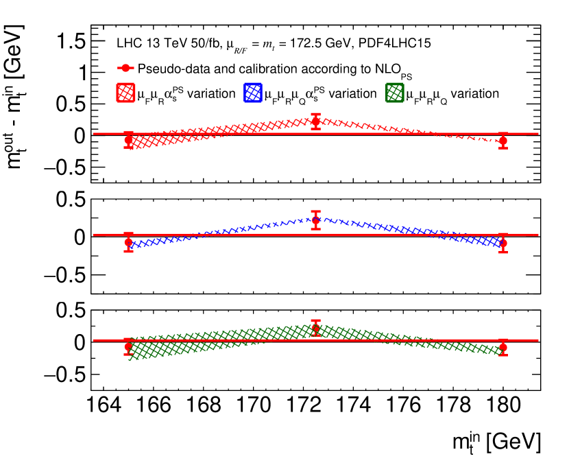
The $m_{lb}$ distributions of the restricted and full showering show clear differences. To quantify the significance of these differences, the parton shower scale uncertainties are assessed. For the decay showers, we performed a decay shower starting scale variation by using factors of $0.5$ and $2.0$ applied to the central scale $\mu_{Q}^{\mathrm{dec}}$. Despite this wide range for varying the resummation scales, we find negligible differences in the shapes of the $m_{lb}$ distributions. Therefore, all variations of the shower description employed here are always based on the fixed value $\mu_{Q}^{\mathrm{dec}}=M_{W}/2$. We use the different schemes described in Section 3.2 to obtain the scale-variation induced theory uncertainties of the $\mathrm{NLO_{PS}}$ prescription presented in Fig. 18(a). While the combined variation, $\mu_{F}\mu_{R}\mu_{Q}{\alpha^{\mathrm{PS}}_{s}}$, leads to the smallest uncertainty band, the band based on the $\mu_{F}\mu_{R}\mu_{Q}$ parameter variation is marginally larger. Most notably, these differences are much smaller than those occurring between the various theory descriptions discussed above.

Finally, for the $\mathrm{NLO_{PS}}$ calculations, we compare in Fig. 18(b) the results for the two central-scale choices $\mu_{R}=\mu_{F}=m_{t}$ and $\mu_{R}=\mu_{F}=\mu_{t\bar{t}}$ as defined in Eq. (15). Although the predicted total cross sections listed in the last two rows of Table 2 depend on this choice, the two predictions lead to consistent measured top quark masses, i.e. the associated offsets agree within their uncertainties.

As can be inferred from Fig. 10(a), the sensitivity of the $m_{lb}$ observable to the top quark mass, and consequently the achievable statistical uncertainty on $m_{t}$ in data, depends on the fit range used. In this context, the range $140$–$160\mathrm{\>GeV}$ is a particularly $m_{t}$-sensitive region, which however also features sizeable differences in the theoretical descriptions, for example as shown in Fig. 2. Consequently, the resulting offsets listed in Table 3 depend on the chosen fit range. As an example, restricting the fit to $m_{lb}<140\mathrm{\>GeV}$ results in absolute differences in the offsets between full range and reduced range of $min=0.05\mathrm{\>GeV}$ and $max=0.36\mathrm{\>GeV}$, where $min$ corresponds to $\mathrm{NLO_{PS}}$ pseudo-data versus $\mathrm{NLO_{NWA}^{NLOdec}}$ calibration, and $max$ corresponds to $\mathrm{NLO_{NWA}^{NLOdec}}$ pseudo-data versus $\mathrm{LO_{NWA}^{LOdec}}$ calibration. In general, larger differences are observed either for larger absolute offsets or for cases with large uncertainty bands. As a result, within the given uncertainties the general pattern does not depend on the fit range. An experimental analysis should be optimised for the smallest total uncertainty, including the variation of the relative importance of statistical and systematic uncertainties, while changing the fit range. Therefore we consider the results shown in Table 3, based on the fit ranges given in Eq. (16), as our nominal values.

		Offset [GeV]		Figure
Pseudo-data	Calibration	$m_{lb}$	$m_{T2}$	$m_{lb}$	$m_{T2}$	$\chi^{2}$
$\mathrm{NLO_{NWA}^{LOdec}}$	$\mathrm{LO_{NWA}^{LOdec}}$	$+0.51\pm 0.06$	$+0.48\pm 0.04$	12(a)	19(a)	0.17
$\mathrm{NLO_{NWA}^{NLOdec}}$	$\mathrm{NLO_{NWA}^{LOdec}}$	$-1.80\pm 0.06$	$-1.67\pm 0.04$	12(b)	19(b)	3.25
$\mathrm{NLO_{NWA}^{NLOdec}}$	$\mathrm{LO_{NWA}^{LOdec}}$	$-1.38\pm 0.07$	$-1.24\pm 0.05$	13(a)	20(a)	2.65
$\mathrm{NLO_{full}}$	$\mathrm{LO_{full}}$	$-1.52\pm 0.07$	$-1.62\pm 0.05$	13(b)	20(b)	1.35
$\mathrm{NLO_{full}}$	$\mathrm{NLO_{NWA}^{NLOdec}}$	$+0.83\pm 0.07$	$+0.60\pm 0.06$	14(a)	21(a)	6.22
$\mathrm{NLO_{full}}$	$\mathrm{NLO_{PS}}$	$-0.09\pm 0.07$	$-0.07\pm 0.06$	14(b)	21(b)	0.05
$\mathrm{NLO_{PS}}$	$\mathrm{NLO_{NWA}^{LOdec}}$	$-0.92\pm 0.07$	$-1.17\pm 0.05$	15(a)	22(a)	8.45
$\mathrm{NLO_{PS}}$	$\mathrm{NLO_{NWA}^{NLOdec}}$	$+0.96\pm 0.07$	$+0.68\pm 0.05$	15(b)	22(b)	10.59
$\mathrm{NLO_{PS}}$	$\mathrm{NLO_{PS}}~{}(\mu_{t\bar{t}})$	$-0.03\pm 0.07$	$+0.02\pm 0.05$	18(b)	25(b)	0.34

Table 3: Summary of the offsets observed when analysing pseudo-data listed in the first column with template fit functions calibrated based on various theoretical predictions as given in the second column. The observed offsets for the two observables $m_{lb}$ and $m_{T2}$ are reported in the second pair of columns, where the corresponding figures are listed in the next pair of columns. Finally, the $\chi^{2}$ for the differences in the offsets for the two observables are displayed in the rightmost column, see text for further details.

4.2 Fit results for $m_{T2}$

The investigations performed for the $m_{lb}$ observable are repeated for $m_{T2}$. The results corresponding to Figs. 12(a) to 18(b) are shown in Figs. 19(a) to 25(b). Also for $m_{T2}$, the offsets obtained when using the corresponding pair of pseudo-data and calibration are consistent with zero, i.e. the method is closed.

While most observations are consistent for the $m_{lb}$ and $m_{T2}$ observables, there are some remarkable differences. For $m_{T2}$, comparing distributions with LO and NLO in production generally results in an $m_{t}$ dependent offset. This indicates that the NLO prediction has a weaker mass dependence than the LO one. The slope of the $m_{lb}$ distribution in Fig. 15 is less steep than the one in Fig. 22. This indicates a different effect of the parton shower on the more inclusive $m_{T2}$, retaining a higher sensitivity to the top quark mass.

The offsets observed for the various pairs of pseudo-data and calibration are given in Table 3. The comparison of the offsets obtained for $m_{T2}$ with those for $m_{lb}$  exhibits a very similar pattern. To investigate whether the sensitivity of the observables to differences in the theoretical predictions coincides, the differences in their offsets are expressed by a $\chi^{2}$ calculated from the offsets, using the fact that the offsets are uncorrelated for their statistical uncertainties. For a number of pairs the differences of the offsets for $m_{lb}$ and $m_{T2}$ are consistent with zero, leading to small values of $\chi^{2}$, for example when comparing $\mathrm{NLO_{NWA}^{LOdec}}$ with $\mathrm{LO_{NWA}^{LOdec}}$ (Figs. 12(a) and 19(a)). In contrast, most notably for the pair $\mathrm{NLO_{PS}}$ and $\mathrm{NLO_{NWA}^{NLOdec}}$ (Figs. 15(b) and 22(b)), the difference is significant, leading to a large $\chi^{2}$. This means, at the expected statistical precision of the $13\mathrm{\>TeV}$ LHC, the two estimators exhibit different sensitivities to this difference in the theoretical prediction.

(a)

(b)

Figure 19: Same as Fig. 12 but for the observable $m_{T2}$.

(a)

(b)

Figure 20: Same as Fig. 13 but for the observable $m_{T2}$.

(a)

(b)

Figure 21: Same as Fig. 14 but for the observable $m_{T2}$.

(a)

(b)

Figure 22: Same as Fig. 15 but for the observable $m_{T2}$.

(a)

(b)

Figure 23: Same as Fig. 16 but for the observable $m_{T2}$.

(a)

(b)

Figure 24: Same as Fig. 17 but for the observable $m_{T2}$.

(a)

(b)

Figure 25: Same as Fig. 18 but for the observable $m_{T2}$.

5 Conclusions

We have studied the impact of various theoretical descriptions for top quark pair production on measurements of the top quark mass in the di-lepton channel. In particular, we have compared the NLO QCD results for $W^{+}W^{-}b\bar{b}$ production ($\mathrm{NLO_{full}}$) to results based on the narrow-width approximation, combining $t\bar{t}$ production at NLO with ($i$) LO top quark decays ($\mathrm{NLO_{NWA}^{LOdec}}$), ($ii$) NLO top quark decays ($\mathrm{NLO_{NWA}^{NLOdec}}$) and ($iii$) a parton shower ($\mathrm{NLO_{PS}}$). We have assessed the theoretical uncertainties associated with the different theory descriptions via the variation of renormalisation, factorisation and shower scales, and investigated the top quark mass sensitivity of the observables $m_{lb}$, $m_{T2}$, $m_{ll}$ and $E_{T}^{\Delta R}$.

Based on these results, we then studied the prospects of a top quark mass extraction from the observables $m_{lb}$ and $m_{T2}$, which we found to be most sensitive to top quark mass variations. Using pseudo-data based on our calculations, we employed the template method to determine the offset in the top quark mass from calibrations that differ in their underlying theory description. These analyses show that the behaviour of the observables $m_{lb}$ and $m_{T2}$ is rather similar in what concerns the observed offsets in the top quark mass.

More importantly, we found that the NLO corrections to the top quark decay play a significant role, because they lead to non-uniform scale uncertainty bands. As the fits are based on normalised differential cross sections, shape differences induced by the scale variations will lead to larger theory uncertainties for the top quark mass extraction. Even though the total scale uncertainties decrease at NLO as to be expected, the shape changes on the $m_{lb}$ distribution induced by scale variations are particularly pronounced in the cases where the decay is described at NLO. For both the $\mathrm{NLO_{full}}$ as well as the $\mathrm{NLO_{NWA}^{NLOdec}}$ description, the theoretical uncertainties in determining $m_{t}$ therefore increase by at least a factor of two compared to the uncertainties emerging when LO decays are involved. Furthermore, the direct comparison of theories differing in their treatment of the top quark decays can lead to offsets of more than $1\mathrm{\>GeV}$ in the measured $m_{t}$ value. This is observed in both cases, i.e. when confronting $\mathrm{NLO_{full}}$ pseudo-data with the $\mathrm{LO_{full}}$ calibration and $\mathrm{NLO_{NWA}^{NLOdec}}$ pseudo-data with the $\mathrm{NLO_{NWA}^{LOdec}}$ calibration. These findings indicate that the non-resonant and non-factorising contributions have a smaller effect on the top quark mass extraction than the NLO treatment of the decay.

Turning to the parton shower ($\mathrm{NLO_{PS}}$) results of our analysis approach, we have compared them to the theory models $\mathrm{NLO_{full}}$ and $\mathrm{NLO_{NWA}^{NLOdec}}$, leading to mass shifts of $-0.09\pm 0.07\mathrm{\>GeV}$ and $0.96\pm 0.07\mathrm{\>GeV}$, respectively (in the $m_{lb}$ case). The good agreement between $\mathrm{NLO_{full}}$ and $\mathrm{NLO_{PS}}$ results can be attributed to the fact that the two descriptions are rather similar for an appropriate fit range, but it does not mean that the two descriptions agree for the entire $m_{lb}$ range. Resummation effects for low $m_{lb}$ values in the $\mathrm{NLO_{PS}}$ case and off-shell effects affecting the tail in the $\mathrm{NLO_{full}}$ case are clearly visible in the $m_{lb}$ distribution. The differences between $\mathrm{NLO_{PS}}$ and $\mathrm{NLO_{NWA}^{NLOdec}}$ mainly originate from the regions of small and near-edge $m_{lb}$ values, where resummation corrections play an important role.

To better understand these differences, we investigated the parton shower behaviour in more detail. We considered results where we limit the number of emissions in both the production and the decay showers, and indeed observe that the predictions of such restricted parton showers move closer to the fixed-order $\mathrm{NLO_{NWA}^{NLOdec}}$ result. These investigations also showed that the resummation corrections incorporated by the unrestricted showers may lead to effects on the top quark mass determination that can be as large as $1\mathrm{\>GeV}$. In addition, we have switched off the shower emissions in either production or decay, and found that both the production and the decay showers impact our analysis in a significant manner. Different ways to assess the shower scale uncertainties within the $\mathrm{NLO_{PS}}$ description were also studied but their effect turned out to be small. The choice of a different central scale also had only a minor impact on the mass determination.

We finally investigated how the choice of the fit range impacts our results and found that the corresponding offsets do not change considerably if the fit range is altered (in a way that still leads to acceptable closure).

Based on our results, we expect that the non-uniform scale variation bands in the $m_{lb}$ distribution, induced by NLO corrections to the decay as present in the $\mathrm{NLO_{full}}$ calculation, would not level out largely if a parton shower was matched to $\mathrm{NLO_{full}}$. It is therefore conceivable that a top quark mass extraction based on LO (or shower approximated) decays may underestimate the theoretical uncertainties, even if higher perturbative orders in the top quark pair production process are taken into account.

In the future, it would be very interesting to see how the pseudo-data used here compare to real data. In this context, the impact of hadronisation and colour reconnection effects should be studied. Owing to the rather strong impact of the resummation, it would also be useful to perform a dedicated comparison of different parton shower prescriptions such as different evolution variables and recoil strategies. Furthermore, it would be worthwhile to investigate how the NLO results for the full $W^{+}W^{-}b\bar{b}$ final state, ideally matched to a parton shower, compare to NNLO results for top quark pair production in the narrow-width approximation, combined with different descriptions of the top quark decay.

References

- (1) M. Czakon, M. L. Mangano, A. Mitov and J. Rojo, Constraints on the gluon PDF from top quark pair production at hadron colliders, JHEP 07 (2013) 167, [1303.7215].
- (2) M. Guzzi, K. Lipka and S.-O. Moch, Top-quark pair production at hadron colliders: differential cross section and phenomenological applications with DiffTop, JHEP 1501 (2015) 082, [1406.0386].
- (3) V. del Duca and E. Laenen, Top physics at the LHC, Int. J. Mod. Phys. A30 (2015) 1530063, [1510.06690].
- (4) M. Czakon, N. P. Hartland, A. Mitov, E. R. Nocera and J. Rojo, Pinning down the large-x gluon with NNLO top-quark pair differential distributions, JHEP 04 (2017) 044, [1611.08609].
- (5) CDF Collaboration, T. Aaltonen et al., Final combination of the CDF results on top-quark mass, CDF note 11080 (2014) .
- (6) D0 collaboration, D0 Collaboration, V.M. Abazov et al., Combination of D0 measurements of the top quark mass, Phys. Rev. D 95 (2017) 112004, [1703.06994].
- (7) ATLAS Collaboration, “Measurement of the top quark mass in the channel from ATLAS data.” ATLAS-CONF-2017-071, 2017.
- (8) CMS collaboration, V. Khachatryan et al., Measurement of the top quark mass using proton-proton data at = 7 and 8 TeV, Phys. Rev. D93 (2016) 072004, [1509.04044].
- (9) ATLAS collaboration, M. Aaboud et al., Measurement of the top quark mass in the dilepton channel from TeV ATLAS data, Phys. Lett. B761 (2016) 350–371, [1606.02179].
- (10) S. Frixione and A. Mitov, Determination of the top quark mass from leptonic observables, JHEP 09 (2014) 012, [1407.2763].
- (11) M. Beneke, P. Marquard, P. Nason and M. Steinhauser, On the ultimate uncertainty of the top quark pole mass, Phys. Lett. B775 (2017) 63–70, [1605.03609].
- (12) M. Butenschoen, B. Dehnadi, A. H. Hoang, V. Mateu, M. Preisser and I. W. Stewart, Top Quark Mass Calibration for Monte Carlo Event Generators, Phys. Rev. Lett. 117 (2016) 232001, [1608.01318].
- (13) S. Kawabata and H. Yokoya, Top-quark mass from the diphoton mass spectrum, Eur. Phys. J. C77 (2017) 323, [1607.00990].
- (14) A. H. Hoang, A. Jain, C. Lepenik, V. Mateu, M. Preisser, I. Scimemi et al., The MSR Mass and the Renormalon Sum Rule, 1704.01580.
- (15) A. H. Hoang, C. Lepenik and M. Preisser, On the Light Massive Flavor Dependence of the Large Order Asymptotic Behavior and the Ambiguity of the Pole Mass, JHEP 09 (2017) 099, [1706.08526].
- (16) A. H. Hoang, S. Mantry, A. Pathak and I. W. Stewart, Extracting a Short Distance Top Mass with Light Grooming, 1708.02586.
- (17) G. Bevilacqua, H. B. Hartanto, M. Kraus, M. Schulze and M. Worek, Top quark mass studies with at the LHC, 1710.07515.
- (18) P. Nason, The Top Mass in Hadronic Collisions, 2017. 1712.02796.
- (19) G. Corcella, R. Franceschini and D. Kim, Fragmentation Uncertainties in Hadronic Observables for Top-quark Mass Measurements, 1712.05801.
- (20) S. Ferrario Ravasio, T. Jezo, P. Nason and C. Oleari, A Theoretical Study of Top-Mass Measurements at the LHC Using NLO+PS Generators of Increasing Accuracy, 1801.03944.
- (21) A. H. Hoang, C. Lepenik and M. Preisser, On the Light Massive Flavor Dependence of the Top Quark Mass, in Proceedings, 13th International Symposium on Radiative Corrections: Application of Quantum Field Theory to Phenomenology (RADCOR2017): St. Gilgen, Austria, September 24-29, 2017, 2018. 1802.04334.
- (22) M. Czakon, D. Heymes and A. Mitov, High-precision differential predictions for top-quark pairs at the LHC, Phys. Rev. Lett. 116 (2016) 082003, [1511.00549].
- (23) M. Czakon, D. Heymes and A. Mitov, Dynamical scales for multi-TeV top-pair production at the LHC, JHEP 04 (2017) 071, [1606.03350].
- (24) M. Czakon, D. Heymes and A. Mitov, fastNLO tables for NNLO top-quark pair differential distributions, 1704.08551.
- (25) M. Czakon, D. Heymes, A. Mitov, D. Pagani, I. Tsinikos and M. Zaro, Top-pair production at the LHC through NNLO QCD and NLO EW, JHEP 10 (2017) 186, [1705.04105].
- (26) W. Hollik and D. Pagani, The electroweak contribution to the top quark forward-backward asymmetry at the Tevatron, Phys. Rev. D84 (2011) 093003, [1107.2606].
- (27) J. H. Kühn, A. Scharf and P. Uwer, Weak Interactions in Top-Quark Pair Production at Hadron Colliders: An Update, Phys. Rev. D91 (2015) 014020, [1305.5773].
- (28) D. Pagani, I. Tsinikos and M. Zaro, The impact of the photon PDF and electroweak corrections on distributions, Eur. Phys. J. C76 (2016) 479, [1606.01915].
- (29) A. Denner and M. Pellen, NLO electroweak corrections to off-shell top-antitop production with leptonic decays at the LHC, JHEP 08 (2016) 155, [1607.05571].
- (30) C. Gütschow, J. M. Lindert and M. Schönherr, Multi-jet merged top-pair production including electroweak corrections, 1803.00950.
- (31) W. Bernreuther, A. Brandenburg, Z. G. Si and P. Uwer, Top quark pair production and decay at hadron colliders, Nucl. Phys. B690 (2004) 81–137, [hep-ph/0403035].
- (32) K. Melnikov and M. Schulze, NLO QCD corrections to top quark pair production and decay at hadron colliders, JHEP 0908 (2009) 049, [0907.3090].
- (33) J. M. Campbell and R. K. Ellis, Top-quark processes at NLO in production and decay, J. Phys. G42 (2015) 015005, [1204.1513].
- (34) M. Brucherseifer, F. Caola and K. Melnikov, corrections to fully-differential top quark decays, JHEP 04 (2013) 059, [1301.7133].
- (35) J. Gao and A. S. Papanastasiou, Top-quark pair-production and decay at high precision, Phys. Rev. D96 (2017) 051501, [1705.08903].
- (36) M. Beneke, P. Falgari, S. Klein and C. Schwinn, Hadronic top-quark pair production with NNLL threshold resummation, Nucl. Phys. B855 (2012) 695–741, [1109.1536].
- (37) M. Cacciari, M. Czakon, M. Mangano, A. Mitov and P. Nason, Top-pair production at hadron colliders with next-to-next-to-leading logarithmic soft-gluon resummation, Phys. Lett. B710 (2012) 612–622, [1111.5869].
- (38) A. Ferroglia, S. Marzani, B. D. Pecjak and L. L. Yang, Boosted top production: factorization and resummation for single-particle inclusive distributions, JHEP 01 (2014) 028, [1310.3836].
- (39) A. Broggio, A. S. Papanastasiou and A. Signer, Renormalization-group improved fully differential cross sections for top pair production, JHEP 10 (2014) 98, [1407.2532].
- (40) N. Kidonakis, High-order threshold corrections for top-pair and single-top production, in Proceedings, Meeting of the APS Division of Particles and Fields (DPF 2015): Ann Arbor, Michigan, USA, 4-8 Aug 2015, 2015. 1509.07848.
- (41) B. D. Pecjak, D. J. Scott, X. Wang and L. L. Yang, Resummed differential cross sections for top-quark pairs at the LHC, Phys. Rev. Lett. 116 (2016) 202001, [1601.07020].
- (42) A. Denner, S. Dittmaier, S. Kallweit and S. Pozzorini, NLO QCD corrections to WWbb production at hadron colliders, Phys. Rev. Lett. 106 (2011) 052001, [1012.3975].
- (43) A. Denner, S. Dittmaier, S. Kallweit and S. Pozzorini, NLO QCD corrections to off-shell top-antitop production with leptonic decays at hadron colliders, JHEP 10 (2012) 110, [1207.5018].
- (44) G. Bevilacqua, M. Czakon, A. van Hameren, C. G. Papadopoulos and M. Worek, Complete off-shell effects in top quark pair hadroproduction with leptonic decay at next-to-leading order, JHEP 02 (2011) 083, [1012.4230].
- (45) G. Heinrich, A. Maier, R. Nisius, J. Schlenk and J. Winter, NLO QCD corrections to production with leptonic decays in the light of top quark mass and asymmetry measurements, JHEP 1406 (2014) 158, [1312.6659].
- (46) A. Denner and M. Pellen, Off-shell production of top-antitop pairs in the lepton+jets channel at NLO QCD, JHEP 02 (2018) 013, [1711.10359].
- (47) R. Frederix, Top Quark Induced Backgrounds to Higgs Production in the Decay Channel at Next-to-Leading-Order in QCD, Phys. Rev. Lett. 112 (2014) 082002, [1311.4893].
- (48) F. Cascioli, S. Kallweit, P. Maierhöfer and S. Pozzorini, A unified NLO description of top-pair and associated Wt production, Eur. Phys. J. C74 (2014) 2783, [1312.0546].
- (49) J. M. Campbell, R. K. Ellis, P. Nason and E. Re, Top-pair production and decay at NLO matched with parton showers, JHEP 04 (2015) 114, [1412.1828].
- (50) P. Nason, A New method for combining NLO QCD with shower Monte Carlo algorithms, JHEP 11 (2004) 040, [hep-ph/0409146].
- (51) S. Frixione, P. Nason and C. Oleari, Matching NLO QCD computations with Parton Shower simulations: the POWHEG method, JHEP 11 (2007) 070, [0709.2092].
- (52) S. Alioli, P. Nason, C. Oleari and E. Re, A general framework for implementing NLO calculations in shower Monte Carlo programs: the POWHEG BOX, JHEP 06 (2010) 043, [1002.2581].
- (53) S. Höche, F. Krauss, P. Maierhöfer, S. Pozzorini, M. Schönherr and F. Siegert, Next-to-leading order QCD predictions for top-quark pair production with up to two jets merged with a parton shower, Phys. Lett. B748 (2015) 74–78, [1402.6293].
- (54) S. Höche, P. Maierhöfer, N. Moretti, S. Pozzorini and F. Siegert, Next-to-leading order QCD predictions for top-quark pair production with up to three jets, Eur. Phys. J. C77 (2017) 145, [1607.06934].
- (55) J. Bellm, K. Cormier, S. Gieseke, S. Plätzer, C. Reuschle, P. Richardson et al., Top Quark Production and Decay in Herwig 7.1, 1711.11570.
- (56) M. V. Garzelli, A. Kardos and Z. Trocsanyi, Hadroproduction of at NLO accuracy matched with shower Monte Carlo programs, JHEP 08 (2014) 069, [1405.5859].
- (57) T. Jezo and P. Nason, On the Treatment of Resonances in Next-to-Leading Order Calculations Matched to a Parton Shower, JHEP 12 (2015) 065, [1509.09071].
- (58) F. Cascioli, P. Maierhöfer and S. Pozzorini, Scattering Amplitudes with Open Loops, Phys. Rev. Lett. 108 (2012) 111601, [1111.5206].
- (59) T. Jezo, J. M. Lindert, P. Nason, C. Oleari and S. Pozzorini, An NLO+PS generator for and production and decay including non-resonant and interference effects, Eur. Phys. J. C76 (2016) 691, [1607.04538].
- (60) L. Buonocore, P. Nason and F. Tramontano, Heavy quark radiation in NLO+PS POWHEG generators, Eur. Phys. J. C78 (2018) 151, [1711.06281].
- (61) R. Frederix, S. Frixione, A. S. Papanastasiou, S. Prestel and P. Torrielli, Off-shell single-top production at NLO matched to parton showers, JHEP 06 (2016) 027, [1603.01178].
- (62) B. Chokoufé Nejad, W. Kilian, J. M. Lindert, S. Pozzorini, J. Reuter and C. Weiss, NLO QCD predictions for off-shell and production and decay at a linear collider, JHEP 12 (2016) 075, [1609.03390].
- (63) ATLAS collaboration, G. Aad et al., Measurement of the top quark mass in the and channels using ATLAS data, Eur. Phys. J. C75 (2015) 330, [1503.05427].
- (64) T. Gleisberg, S. Höche, F. Krauss, M. Schönherr, S. Schumann, F. Siegert et al., Event generation with SHERPA 1.1, JHEP 02 (2009) 007, [0811.4622].
- (65) G. Cullen, N. Greiner, G. Heinrich, G. Luisoni, P. Mastrolia, G. Ossola et al., Automated One-Loop Calculations with GoSam, Eur. Phys. J. C72 (2012) 1889, [1111.2034].
- (66) G. Cullen et al., GS-2.0: a tool for automated one-loop calculations within the Standard Model and beyond, Eur. Phys. J. C74 (2014) 3001, [1404.7096].
- (67) T. Binoth et al., A Proposal for a standard interface between Monte Carlo tools and one-loop programs, Comput. Phys. Commun. 181 (2010) 1612–1622, [1001.1307].
- (68) S. Alioli et al., Update of the Binoth Les Houches Accord for a standard interface between Monte Carlo tools and one-loop programs, Comput. Phys. Commun. 185 (2014) 560–571, [1308.3462].
- (69) A. Denner and S. Dittmaier, The Complex-mass scheme for perturbative calculations with unstable particles, Nucl. Phys. Proc. Suppl. 160 (2006) 22–26, [hep-ph/0605312].
- (70) S. Höche, F. Krauss, M. Schönherr and F. Siegert, A critical appraisal of NLO+PS matching methods, JHEP 09 (2012) 049, [1111.1220].
- (71) S. Höche, J. Huang, G. Luisoni, M. Schönherr and J. Winter, Zero and one jet combined next-to-leading order analysis of the top quark forward-backward asymmetry, Phys. Rev. D88 (2013) 014040, [1306.2703].
- (72) S. Höche, S. Kuttimalai, S. Schumann and F. Siegert, Beyond Standard Model calculations with Sherpa, Eur. Phys. J. C75 (2015) 135, [1412.6478].
- (73) K. Hamilton and P. Richardson, A Simulation of QCD radiation in top quark decays, JHEP 02 (2007) 069, [hep-ph/0612236].
- (74) C. G. Lester and D. J. Summers, Measuring masses of semiinvisibly decaying particles pair produced at hadron colliders, Phys. Lett. B463 (1999) 99–103, [hep-ph/9906349].
- (75) A. Barr, C. Lester and P. Stephens, m(T2): The Truth behind the glamour, J. Phys. G29 (2003) 2343–2363, [hep-ph/0304226].
- (76) ATLAS collaboration, Measurement of lepton differential distributions and the top quark mass in production in collisions at TeV with the ATLAS detector, Tech. Rep. ATLAS-CONF-2017-044, CERN, Geneva, Jul, 2017.
- (77) J. Butterworth et al., PDF4LHC recommendations for LHC Run II, J. Phys. G43 (2016) 023001, [1510.03865].
- (78) S. Dulat, T.-J. Hou, J. Gao, M. Guzzi, J. Huston, P. Nadolsky et al., New parton distribution functions from a global analysis of quantum chromodynamics, Phys. Rev. D93 (2016) 033006, [1506.07443].
- (79) L. A. Harland-Lang, A. D. Martin, P. Motylinski and R. S. Thorne, Parton distributions in the LHC era: MMHT 2014 PDFs, Eur. Phys. J. C75 (2015) 204, [1412.3989].
- (80) NNPDF collaboration, R. D. Ball et al., Parton distributions for the LHC Run II, JHEP 04 (2015) 040, [1410.8849].
- (81) M. Jezabek and J. H. Kühn, Semileptonic Decays of Top Quarks, Phys. Lett. B207 (1988) 91–96.
- (82) M. Cacciari, G. P. Salam and G. Soyez, The Anti-k(t) jet clustering algorithm, JHEP 04 (2008) 063, [0802.1189].
- (83) M. Cacciari, G. P. Salam and G. Soyez, FastJet User Manual, Eur. Phys. J. C72 (2012) 1896, [1111.6097].
- (84) A. A. Maier, Precision Measurements of the Top Quark Mass in the Dileptonic Top Quark Pair Decay Channel at ATLAS , PhD thesis, Max Planck Institute for Physics, Munich, Germany, https://publications.mppmu.mpg.de/2016/MPP-2016-76/FullText.pdf.