An adaptive reduced basis collocation method based on PCM ANOVA decomposition for anisotropic stochastic PDEs

Abstract

The combination of reduced basis and collocation methods enables efficient and accurate evaluation of the solutions to parameterized PDEs. In this paper, we study the stochastic collocation methods that can be combined with reduced basis methods to solve high-dimensional parameterized stochastic PDEs. We also propose an adaptive algorithm using a probabilistic collocation method (PCM) and ANOVA decomposition. This procedure involves two stages. First, the method employs an ANOVA decomposition to identify the effective dimensions, i.e., subspaces of the parameter space in which the contributions to the solution are larger, and sort the reduced basis solution in a descending order of error. Then, the adaptive search refines the parametric space by increasing the order of polynomials until the algorithm is terminated by a saturation constraint. We demonstrate the effectiveness of the proposed algorithm for solving a stationary stochastic convection-diffusion equation, a benchmark problem chosen because solutions contain steep boundary layers and anisotropic features. We show that two stages of adaptivity are critical in a benchmark problem with anisotropic stochasticity.

1 Introduction

Numerical methods for high-dimensional anisotropic parameterized partial differential equations (PDEs) have received increasing interest in various areas of science and engineering. These problems are costly to solve because of requirements of high fidelity in space or high dimensionality in the parameterized random space. This study concerns some new approaches for reducing costs, by combining reduced basis methods for the spatial component of the problem with specialized quadrature rules for the parameterized component.

An approach to reduce spatial complexity is reduced basis methods, developed to cope with parameterized systems that require repeated use of a high-fidelity solver. Costly computations for high-resolution solutions for multiple parameter values are replaced by an approach with lower complexity, which computes parameterized solutions with a cost that is independent of the dimension of the original problem [19, 28, 29, 32, 33, 27, 30, 2, 21]. Instead of solving the full discrete PDE system, a cheaper system is obtained by a projection into a lower-dimensional parametric space determined by the full-system solution at a distinguished set of parameters. Convergence analysis is available for various types of PDEs [27, 31, 33] using so-called certified reduced basis methods. Extension to parameterized stochastic PDEs is straightforward [8, 7], and applications in stochastic control [6] have been studied as well.

The two components of reduced basis methods are referred to as an offline step (construction of the reduced space by computation of required full-system solutions) and an online step (computations on the reduced space) designed to be cheap. In addition to requirements of spatial resolution, the other contribution to cost comes from the high dimensionality of the stochastic space. In order to parametrize noisy input data for a given PDE, random fields can often be expanded as an infinite combination of random variables by, for instance, Karhunen-Loève [15, 26] or polynomial chaos [40, 41] expansions. Such random fields can be well approximated using a finite number of variables [34], but the dimensionality may be high. For such high dimensions in the stochastic space, high-dimensional integration techniques [3, 16], based for example on Smolyak sparse-grid [22, 24] or ANOVA decomposition [36, 5, 13], can be employed to compute the statistical moments of the solution. Although these methods are often efficient compared to Monte-Carlo methods, the curse of dimensionality remains a challenge. Thus, new ideas are necessary to increase efficiency and facilitate rapid evaluation of quantities of interest.

The idea of reduced basis methods combined with high-dimensional collocation schemes [10] brings the aforementioned efforts together. Instead of searching arbitrary samples, the candidate reduced basis points are chosen to be the sparse-grid probabilistic collocation points. If the solution vector is not of full rank in the parametric space, the computational cost can be reduced with essentially no loss of accuracy. However, the online stage involves a cost that is proportional to the number of collocation points. Thus, the algorithm suffers from the curse of dimensionality with costs that are less than for using the full collocation scheme, but still depending on the stochastic dimensionality. This cost can be further reduced by using dimension adaptation approaches, for instance, anisotropic sparse-grid [7] and ANOVA decomposition [18, 20].

In this paper, we study the reduced basis collocation method for stochastic PDEs, and propose an adaptive procedure both in the dimensions of the stochastic space and the degrees of freedom in each parametric direction. An outline of the paper is as follows. In section 2, we review the reduced basis collocation method based on ANOVA collocation methods and examine the quality of different interpolation points. Then, we introduce the adaptive ANOVA procedure employed in the reduced basis algorithm, emphasizing its advantage for reducing computational cost and automatic sorting. Then, in section 3, we propose an adaptive reduced basis algorithm based on a probabilistic collocation method (PCM). In addition to the adaptive dimension procedure described in section 2, resolution in the parametric space is managed by adapting the polynomial order $p$ discussed in section 3. We test these ideas on the stationary stochastic convection-diffusion equation chosen as a benchmark problem because of its interesting features such as solutions with steep boundary layers and discontinuities. The reduced basis ANOVA approach is suitable to study the interaction of these characteristics with the underlying noise that yields anisotropy in the stochastic space.

2 Reduced basis collocation methods based on ANOVA decomposition

In this section, we review the reduced basis approximation for the solution computed using collocation in the stochastic space. Consider a stochastic problem consisting of a partial differential operator $\mathcal{L}$ and a boundary operator $b$,

$$\mathcal{L}(x,\omega,u(x,\omega))=f(x),\quad^{\forall}x\in D,$$ (1)

$$b(x,\omega,u(x,\omega))=g(x),\quad^{\forall}x\in\partial D,$$

on $D\times\Omega$, where $D\subset\mathbb{R}^{d}$ is the spacial domain, assumed to be a bounded and connected domain with polygonal boundary $\partial D$, and $\Omega$ is a complete probability space of $(\Omega,\Sigma,\mathcal{P})$ with $\sigma$-algebra $\Sigma$ and probability measure $\mathcal{P}$. Assume that the stochastic excitation can be represented by a finite number of random variables $\xi=[\xi_{1},...,\xi_{M}]^{T}$ on $\Gamma=\prod_{m=1}^{M}\Gamma_{m}$, where $\Gamma_{m}=[a_{m},\,b_{m}]$ is the image of $\xi_{m}(\omega)$. This could come from a variety of sources, for example, a truncated Karhunen-Loève (KL) expansion [15, 26], a partitioning of $D$ into subdomains, or uncertain boundary conditions.

In this paper, we consider the steady-state convection-diffusion equation,

$$-\nabla\cdot a(x,\xi)\nabla u(x,\xi)+w\cdot\nabla u(x,\xi) = f(x)\quad\,\textrm{ in }\,\,\quad D\times\Gamma$$ (2)

$$u(x,\xi) = g_{D}(x)\quad\,\textrm{ on }\,\,\partial D\times\Gamma$$

where $a(x,\xi)$ is a parametrized random diffusion coefficient, $w$ is a constant convective velocity, and $f(x)$ is the forcing term. The boundary conditions are imposed as Dirichlet conditions with $g_{D}(x)$. We will consider choices of $a(x,\xi)$ and $g_{D}(x)$ that involve discontinuity. The stochasticity in the diffusion coefficient $a(x,\xi)$ is taken as a piecewise constant function on partitions, i.e., $D$ is divided into $N_{D}$ equal-sized subdomains of horizontal strips, squares, or vertical strips. Figure 1 shows three examples for $N_{D}=16$, namely, $1\times 16$, $4\times 4$, and $16\times 1$, on $D=[-1,\,1]\times[-1,\,1]$. On each subdomain, we consider

$$a(\cdot;\xi)|_{D_{m}}=\nu\,\xi_{m},\quad m=1,...,N_{D},$$ (3)

with a constant $\nu$ and random variables $\{\xi_{m}\}_{m=1}^{N_{D}}$. The dimensionality of the random space is identical to the number of subdomains, $M=N_{D}$. The boundary conditions are imposed as Dirichlet conditions with

$$g_{D}(x_{1},x_{2})=\begin{cases}1,\quad x\in\{x\in\partial D|x_{1}=-1\}\cup\{x\in\partial D|-1\leq x_{1}\leq 0,x_{2}=-1\}.\\ 0,\quad\textrm{ otherwise }\end{cases}.$$ (4)

The conditions yield jump discontinuities at the points $(0,\,-1)$ and $(-1,\,1)$.

Examples of solutions to this system with a constant convective velocity $w=\left(\sin(\pi/6),\,\cos(\pi/6)\right)$ and a constant forcing $f=1$ are shown in Figure 2. The mean and standard deviation are plotted for the case of $N_{D}=4$ with a $2\times 2$ partition and uniform random variables $\{\xi_{m}\}_{m=1}^{N_{D}}$ on $\Gamma_{m}=[0.01,\,1]$ with diffusion parameter $\nu=1/2$ and $1/20$. There is an exponential boundary layer near the top boundary $x_{2}=1$. The discontinuity from the boundary condition is smeared by the presence of diffusion, producing an internal layer. In addition, the standard deviation is less regular on the edges of the subdomains associated with $a(\cdot,\cdot)$. The diffusion coefficient lies in the range $[0.01\nu,\nu]$, and the images on the right show results for a smaller diffusion parameter $\nu=1/20$. For this case, the overall variance on the domain tends to be smaller than for $\nu=1/2$, but the magnitude is larger in a narrow region near the top boundary layer. We will further study the impact of randomness on each subdomain on the irregular features of the solution using the reduced basis method combined with ANOVA decomposition. This approach will reveal the effects of the anisotropic nature of the problem and show the effectiveness of the method for anisotropic systems while obtaining good spatial resolution with a reasonable amount of computational cost.

    $1\times 16$                            $4\times 4$                            $16\times 1$

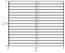
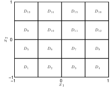
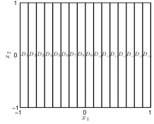
Figure 1: Examples of subdomains for test problem (3) of horizontal strips, squares, and vertical strips with $N_{D}=16$.

       $2\times 2$, $\quad\nu=1/2$                                                      $2\times 2$, $\quad\nu=1/20$

$\mathrm{E}[u(x)]$                             $\sigma[u(x)]$                           $\mathrm{E}[u(x)]$                             $\sigma[u(x)]$

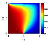
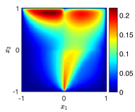
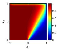
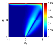
Figure 2: Examples of mean $\mathrm{E}[u(x)]$ and standard deviation $\sigma[u(x)]$ for diffusion parameter $\nu=1/2$ and $\nu=1/20$ on $2\times 2$ partition.

2.1 Collocation methods

Collocation methods approximate the solution by interpolation at a set of Lagrange polynomials at collocation points,

$$u\left(x,\,\xi\right)\approx\sum_{\xi^{(k)}\in\Theta}u_{c}\left(x,\xi^{(k)}\right)L_{\xi^{(k)}}(\xi),$$ (5)

where $\Theta\subset\Gamma$ is a finite sample set (the collocation points), $\{L_{\xi^{(k)}}(\xi)\}$ are the Lagrange interpolation polynomials on $\Gamma$, and the coefficient function $u_{c}\left(x,\xi^{(k)}\right)$ is the solution of a deterministic problem corresponding to a given realization $\xi^{(k)}$ of the random vector $\xi$. We denote the weak form of the system (2) at a given realization $\xi$ as $B_{\xi}(u(\cdot,\xi),v)=l(v)$, where

$$B_{\xi}(u,v)\doteq\int_{D}\left(a\nabla u\cdot\nabla v+(w\cdot\nabla u)v\right)dx,\quad l(v)\doteq\int_{D}fv\,dx,$$ (6)

Let $X_{\mathsf{h}}$ be a finite-dimensional finite element space of dimension $N_{\mathsf{h}}=O({1}/{\mathsf{h}^{d}})$ defined on $D\subset\mathbb{R}^{d}$, where $\mathsf{h}$ is a grid parameter of the spatial domain. We consider a quadrilateral finite element space with the streamline diffusion method [12] to enhance stability when boundary layers are present. Nonhomogeneous boundary conditions are interpolated using addition basis functions at the boundary. Then the finite element solution $u_{\mathsf{h}}(\cdot,\xi)\in X_{\mathsf{h}}$ can be computed as

$$B_{\xi}^{(sd)}(u_{\mathsf{h}}(\cdot,\xi),v)=l(v),\quad^{\forall}v\in X_{\mathsf{h}}.$$ (7)

where $B_{\xi}^{(sd)}$ incorporates streamline-diffusion terms (see [12], section 6.3 for details). For fixed $\xi$, we refer to this sample solution as a snapshot. Given a finite set of parameters $\Theta$, we can gather all the snapshots computed on $\Theta$ as

$$S_{\Theta}\doteq\{u_{\mathsf{h}}(\cdot,\xi),\,\xi\in\Theta\}.$$ (8)

This can be associated with a matrix $\mathbf{S}_{\Theta}\in\mathbb{R}^{N_{\mathsf{h}}\times|\Theta|}$, where each column of $\mathbf{S}_{\Theta}$ is a vector of coefficients of basis functions of the finite element solution. Here, we assume that the finite element approximation is sufficiently fine so that the spatial discretization error is acceptable.

The full collocation solution (8) can be computed by applying a deterministic solver $|\Theta|$ times. If $\Theta$ consists of a full tensor product of one-dimensional parameter values, i.e., $\Theta=\Theta_{1}^{i_{1}}\otimes\cdots\otimes\Theta_{M}^{i_{M}}$, where $\Theta_{m}^{i_{m}}$ is the set of collocation points in the $m$-th direction of order $i_{m}$, costs grow exponentially with respect to the dimension $M$. The sparse-grid collocation method [16, 24, 22, 3] reduces this cost using a subset of the full tensor grid collocation points

$$\Theta_{\ell}=\cup_{\ell+1\leq|\mathbf{i}|\leq\ell+M}\left(\Theta_{1}^{i_{1}}\otimes\cdots\otimes\Theta_{M}^{i_{M}}\right),$$

where $|\mathbf{i}|=i_{1}+\cdots+i_{M}$ and the level $\ell$ is the parameter that truncates the level of interaction. The choice of sparse-grid collocation points are typically taken to be nodes used for quadrature in $M$-dimensional space. The most common ones are Clenshaw-Curtis and Gauss abscissae. The convergence behavior of the reduced basis collocation method using Clenshaw-Curtis quadrature is studied in [10]. Here, we compare Clenshaw-Curtis and Gauss-Legendre points used in the reduced basis collocation method that will be described later. Figure 3 shows the error in the moments with respect to the size of the reduced basis $N_{r}$. It is evident that the choice of the interpolation point is critical and Gauss-Legendre is the more effective choice for this example. In the sequel, we restrict our attention to Gauss-Legendre quadrature.

        $1\times 4$                          $4\times 1$                          $1\times 16$                          $16\times 1$

mean

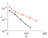
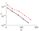
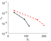
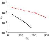
s.d.

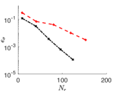
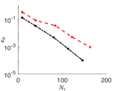
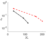
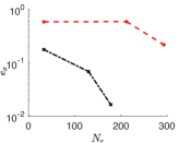
Figure 3: Comparison of Clenshaw-Curtis (CC) and Gauss-Legendre (GL) sparse-grid points in the reduced basis method. The plots compare relative $L_{2}$-error in the mean and standard deviation versus the size of reduced basis $N_{r}$ for the problem with $\nu=1/2$. The results are computed with Algorithm 1 while increasing the sparse-grid level from $\ell=1$ to $5$ using tolerance $\epsilon_{RB}=10^{-5}$ when $N_{D}=4$, and from $\ell=1$ to $3$ with $\epsilon_{RB}=10^{-4}$ when $N_{D}=16$.

2.2 ANOVA decomposition for collocation methods

An alternative to sparse-grid collocation uses an ANOVA decomposition of an $M$-dimensional function. This decomposition has the form

$$u(\,\cdot,\,\xi_{1},...,\xi_{M}) = {u}_{0}(\cdot)+\sum_{j_{1}=1}^{M}{u}_{j_{1}}(\,\cdot,\,\xi_{j_{1}})+\sum_{j_{1}<j_{2}}^{M}{u}_{j_{1}j_{2}}(\,\cdot,\,\xi_{j_{1}},\xi_{j_{2}})+\cdots$$ (9)

This representation decomposes multivariate functions according to the degree of interaction among the variables. For instance, ${u}_{j_{1}j_{2}}(\,\cdot,\,\xi_{j_{1}},\xi_{j_{2}})$ describes the second-order or two-body interaction between the variables $\xi_{j_{1}}$ and $\xi_{j_{2}}$. Similar to sparse-grid collocation, by truncating the series at a certain level, an $M$-dimensional function can be approximated using a function on a lower-dimensional subspace of the $M$-dimensional parameter space. Such a decomposition can be computed by ${u}_{K}(\,\cdot,\,\xi_{K})\doteq\int_{\Gamma_{K^{\prime}}}u(\,\cdot,\,\xi)d\mu(\xi_{K^{\prime}})-\sum_{S\subset K}{u}_{T}(\,\cdot,\,\xi_{S})$, where $K\subset\{1,\cdots,M\}$ and $K^{\prime}$ is the complement of $K$ in $\{1,\cdots,M\}$.

This construction can be put in a form similar to that of collocation by replacing the Lebesgue measure with a Dirac measure $d\mu=\delta(\xi-\mathbf{c})$. This is called the anchored-ANOVA method where $\mathbf{c}$ is the anchor point [13, 36]. The first few terms in the anchored-ANOVA decomposition become ${u}_{0}(\cdot)=u(\,\cdot,\,\mathbf{c})=u(\,\cdot,\,c_{1},\cdots,c_{M})$, ${u}_{j}(\,\cdot,\,\xi_{j})=u(\,\cdot,\,c_{1},..,\xi_{j},..,c_{M})-{u}_{0}(\cdot)$, and ${u}_{ij}(\,\cdot,\,\xi_{i},\xi_{j})=u(\,\cdot,\,c_{1},..\xi_{i},..,\xi_{j},..,c_{M})-{u}_{i}(\,\cdot,\,\xi_{i})-{u}_{j}(\,\cdot,\,\xi_{j})-{u}_{0}(\cdot)$. By considering the ANOVA approximation in the random space discretized by the probabilistic collocation method (PCM) [1, 39] in each parametric space, the solution approximated up to level $\ell$ can be written as

$$u(\cdot,\xi)=\sum_{K\subset\{1,...,M\},|K|\leq\ell}\varkappa_{M,|K|,\ell}\left[\sum_{\xi^{(k)}\in\Xi_{K}^{p}}u_{K}\left(\cdot,\xi^{(k)}\right)L_{\xi^{(k)}}(\xi)\right],$$ (10)

where $\varkappa_{M,|K|,\ell}$ is a signed number counting the frequency of the sample solutions at $\xi^{(k)}\in\Xi_{K}^{p}$ appearing in the ANOVA expansion up to level $\ell$, that is, $\varkappa_{M,j,\ell}=\sum_{r=j}^{\ell}\left(-1\right)^{r-j}\frac{(M-j)!}{(r-j)!(M-r)!}$ and $\Xi_{K}^{p}$ is the set of PCM-ANOVA collocation points [13, 44] in direction $K$ up to polynomial order $p$ for all the parameters. For instance, if $\{\xi_{m}^{\kappa_{m}}\}_{\kappa_{m}=1}^{p_{m}}$ are the PCM points in the $m$-th parameter of polynomial order $p_{m}$, then

$$\Xi_{1}^{p_{1}} = \{(\xi_{1}^{\kappa_{1}},c_{2},...,c_{M})\in\Gamma\,|\,1\leq\kappa_{1}\leq{p_{1}}\},$$ (11)

$$\Xi_{(1,2)}^{(p_{1},p_{2})} = \{(\xi_{1}^{\kappa_{1}},\xi_{2}^{\kappa_{2}},c_{3},...,c_{M})\in\Gamma\,|\,1\leq\kappa_{1}\leq{p_{1}},\,1\leq\kappa_{2}\leq{p_{2}}\}.$$

We denote the set of collocation points up to level $\ell$ and its size as

$$\Xi_{\ell}\doteq\cup_{|K|\leq\ell}\Xi_{K}^{p},\qquad C(M,\ell)\doteq|\Xi_{\ell}|=\sum_{l=0}^{\ell}\left(\begin{matrix}M\\ l\end{matrix}\right)p^{l},$$ (12)

respectively. For stochastic problems, it was shown in [23] that an ANOVA decomposition of level two has good accuracy if the anchor point is chosen as the mean of the probability density function considered, and we will use this technique.

An error indicator for the ANOVA truncation can be constructed using the relative size of either the mean or variance in each term [42, 22]. In our work, we take the ANOVA indicator for the $K$-th term using the mean as

$$\gamma_{K}\doteq\frac{\|\mathrm{E}[{u}_{K}]\|}{\sum_{|S|<|K|}\|\mathrm{E}[{u}_{S}]\|}.$$ (13)

2.3 Reduced basis collocation method

Reduced basis algorithms aim to reduce the computational cost by approximating the solution using full discrete solutions computed only on a small subset of parameters $\Theta_{r}\subset\Xi_{\ell}$. Let $N_{r}\doteq|\Theta_{r}|$. The goal is to find a set of finite element solutions $Q=\{q_{1},\cdots,q_{N_{r}}\}$ computed on $\Theta_{r}$ that give an accurate representation of the column space of $\mathbf{S}_{\Xi_{\ell}}$. Such an approximate solution $u_{rb}(\cdot,\xi)\in span(Q)$ satisfies

$$B_{\xi}\left(u_{rb}(\cdot,\xi),v\right)=l(v),\quad^{\forall}v\in span(Q).$$ (14)

The size $N_{r}$ of the reduced problem (14) is typically much smaller than $N_{\mathsf{h}}$ from (7), and the utility of reduced basis methods derives from this fact [27, 31]. Here we summarize the procedure.

Assume that the operator $\mathcal{L}$ is linear and is affinely dependent on the vector of parameters $\xi$, that is, $\mathcal{L}=\sum_{i=1}^{\hat{n}_{a}}\phi_{i}(\xi)\mathcal{L}_{i}$. Then, the weak form (7) requires solution of a linear system of order $N_{\mathsf{h}}$,

$$\mathbf{A}_{\xi}\mathbf{u}_{\xi}=\mathbf{f},$$ (15)

where $\mathbf{A}_{\xi}=\sum_{i=1}^{\hat{n}_{a}}\phi_{i}(\xi)\mathbf{A}_{i}$, and $\mathbf{A}_{i}$ are parameter-independent matrices. For each $q_{i}\in Q$, let $\mathbf{q}_{i}$ denote the vector of coefficients associated with $q_{i}$. Then $\mathbf{Q}=[\mathbf{q}_{1},\cdots,\mathbf{q}_{N_{r}}]\in\mathbb{R}^{N_{h}\times N_{r}}$ is the matrix representation of $Q$, and the linear system obtained from a Galerkin condition corresponding to the reduced problem (14) can be written as

$$\mathbf{Q}^{T}\mathbf{A}_{\xi}\mathbf{Q}\widetilde{\textbf{u}}_{\xi}=\sum_{i=1}^{\hat{n}_{a}}\phi_{i}(\xi)\left(\mathbf{Q}^{T}\mathbf{A}_{i}\mathbf{Q}\right)\widetilde{\textbf{u}}_{\xi}=\mathbf{Q}^{T}\mathbf{f},$$ (16)

where $\mathbf{Q}\widetilde{\textbf{u}}_{\xi}$ is the reduced basis solution approximating $\mathbf{u}_{\xi}$. If the parameter-independent quantities $\mathbf{Q}^{T}\mathbf{A}_{i}\mathbf{Q}$ and $\mathbf{Q}^{T}\mathbf{f}$ are precomputed, the cost to assemble the reduced system for each $\xi$ becomes $O(N_{r}^{2})$ times $\hat{n}_{a}$. The reduced basis algorithm computed with collocation points $\Theta$ is summarized in Algorithm 1. Either sparse-grid or ANOVA collocation can be employed by updating the reduced basis matrix while increasing the level from $0$ to $\ell$, that is, $\mathbf{Q}$ = RBM($\mathbf{Q}$, $\Xi_{l}$, $\epsilon$), for $0\leq l\leq\ell$ (see [10, 20] for details). Here, $\epsilon_{RB}$ is an acceptance tolerance for the reduced basis solution based on an error indicator. We use a residual based error indicator,

$$\eta_{Q,\xi^{(k)}}\doteq\frac{\|\mathbf{A}_{\xi^{(k)}}\mathbf{Q}\widetilde{\textbf{u}}_{\xi^{(k)}}-\mathbf{f}\|_{2}}{\|\mathbf{f}\|_{2}}w^{(k)},$$ (17)

where $w^{(k)}=\mathbb{P}(\xi=\xi^{(k)})^{\alpha}$, $0\leq\alpha\leq 1$ [38, 6]. An alternative error indicator is a dual-based indicator developed in [33, 27], which depends on having an a posteriori error estimate for the associated problem.

   1: for   $1\leq k\leq|\Theta|$ do

   2:     Compute $\widetilde{\textbf{u}}_{\xi^{(k)}}$ by solving (14) and the error indicator $\eta_{\mathbf{Q},\xi^{(k)}}$ of (17).

   3:     if   $\eta_{\mathbf{Q},\xi^{(k)}}<\epsilon_{RB}$ then

   4:        Use the reduced solution $u_{R}(\cdot,\xi^{(k)})=\mathbf{Q}\widetilde{\textbf{u}}_{\xi^{(k)}}$ to serve as $u_{c}(\cdot,\xi^{(k)})$ in (5).

   5:     else

   6:        Compute the full solution vector $\mathbf{u}_{\xi^{(k)}}$ by solving (15).

   7:        Use $u_{h}(\cdot,\xi^{(k)})$ derived from $\mathbf{u}_{\xi^{(k)}}$ to serve as $u_{c}(\cdot,\xi^{(k)})$ in (5).

   8:        Update $\mathbf{S}_{\Theta_{r}}$ and $\mathbf{Q}$ by augmenting $\mathbf{u}_{\xi^{(k)}}$ and the orthogonal complement.

   9:        Reconstruct the offline reduced matrices and vectors, $\mathbf{Q}^{T}\mathbf{A}_{i}\mathbf{Q}$, $\mathbf{Q}^{T}\mathbf{f}$, $\mathbf{Q}^{T}\mathbf{A}_{i}\mathbf{A}_{j}\mathbf{Q}$, and $\mathbf{Q}^{T}\mathbf{A}_{i}\mathbf{f}$.

10:     end

11: end

Algorithm 1 $(\mathbf{Q},\,\mathbf{S}_{\Theta_{r}})$ = RBM($\mathbf{Q}$, $\Theta$, $\epsilon_{RB}$) : Reduced basis algorithm to update the reduced basis matrix $\mathbf{Q}$ considering the collocation points $\Theta$ and tolerance $\epsilon_{RB}$.

The total cost of a reduced basis algorithm can be divided into two parts as

$$C(M,\ell)\cdot(\textit{cost of reduced system solves and residual calculation})+\hskip 11.38092pt$$ (18)

$$N_{r}\cdot(\textit{cost of full system solves and construction of offline quantities}),$$

where the former and latter terms are on the order of $N_{r}$ and $N_{h}$, respectively. Here, $C(M,\ell)$ is the number of sparse-grid nodes or ANOVA collocation points. The efficiency of the reduced basis algorithm comes from avoiding the full system solve on some collocation points. However, the cost becomes large as $M$ and $\ell$ increase. Dimension-adaptive approaches can further improve the efficiency for anisotropic problems. The ANOVA indicator $\gamma_{K}$ (13) can be used to select only the important directions. After each level $l$, we choose the ANOVA terms $u_{K}$ (10) such that $\gamma_{K}$ is greater than a tolerance $\epsilon_{A}$, and refer to the component of these terms as the effective dimensions $\mathcal{J}_{l}$, i.e.,

$$\mathcal{J}_{l}=\{|K|=l\,|\,\gamma_{K}>\epsilon_{A}\}.$$ (19)

We use these indices to build the next level ANOVA approximation (see lines 19–20 of Algorithm 3 for details). The number of search points is reduced to $C(\widetilde{M},\ell)$, where $\widetilde{M}$ is the number of the effective dimensions. This is a standard procedure in adaptive ANOVA schemes [42, 22] and has been studied in the context of reduced basis methods in [20, 18].

Here, we emphasize that we also employ the ANOVA indicator $\gamma_{K}$ (13) to sort the search direction $\mathcal{J}_{\ell}$ and the newly added reduced basis solution $\mathbf{S}_{N_{r}}$. Both are sorted in each level according to the descending order of $\gamma_{K}$. Since the ANOVA indicator implies the priority of the reduced basis, this procedure enhances the quality of the reduced basis and saves the additional cost that occurs from sorting the reduced basis afterwards.

   1: Initialize $\mathbf{S}=[\,]$ and $\mathcal{J}=[\,]$.

   2: while   $\mathcal{J}_{\ell}\neq\emptyset$ do

   3:     Find the index with the maximum ANOVA indicator $L=\arg\max\{\gamma_{K}\,|\,K\in\mathcal{J}_{\ell}\}$.

   4:     Save the sorted reduced basis $\mathbf{S}=[\mathbf{S},\mathbf{S}_{L}]$ and ANOVA index $\mathcal{J}=[\mathcal{J},L]$.

   5:     $\mathcal{J}_{\ell}=\mathcal{J}_{\ell}\backslash L$.

   6: end

Algorithm 2 $(\mathbf{S},\mathcal{J})$ = RB-Sort($\{\gamma_{K}\}$, $\{\mathbf{S}_{K}\}$, $\mathcal{J}_{\ell}$) : Sort the reduced basis and ANOVA index in the descending order of ANOVA indicator $\gamma_{K}$.

2.4 Numerical results

In this section, we use the reduced basis algorithm based on ANOVA to examine the features of the benchmark problem (2) and the accuracy of the method. We consider the spatial domain $D=[-1,1]\times[-1,1]$, with the system parameters described in the beginning of section 2. We take the random variables $\xi_{m}$ in the piecewise constant diffusion coefficient $a(x,\xi)$ of (3) to be independent and uniformly distributed on $\Gamma_{m}=[0.01,\,1]$. The magnitude of the diffusion parameter $\nu$ is either $1/2$ or $1/20$ for examples of moderate and small diffusion. We choose the convective velocity $w$ to correspond to a 30-degree angle right of vertical, and the Dirichlet boundary condition $g_{D}(x_{1},x_{2})$ as in (4). For each sample point, we find a weak discrete solution $u_{h}(x,\xi)\in X_{\mathsf{h}}$. For the finite element discretization of $D$, we use a bilinear ($Q_{1}$) finite element approximation [4]. The deterministic solver is based on the IFISS software package [11, 35] and the spatial discretization is done on a uniform $128\times 128$ grid, so that $N_{\mathsf{h}}=128^{2}$.

  

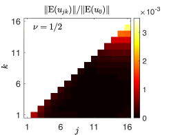
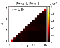
Figure 4: Relative magnitudes of means of the first and second order ANOVA expansion terms $u_{j}(x,\xi_{j})$ and $u_{jk}(x,\xi_{j},\xi_{k})$ in the case of $1\times 16$ subdomain, comparing $\nu=1/2$ and $\nu=1/20$. The solution for the example with smaller diffusion parameter $\nu=1/20$ is more anisotropic but has smaller variance.

To explore accuracy with respect to parameterization, we compute a reference solution using a quasi Monte-Carlo (MC) method with $10^{5}$ samples of a Halton sequence, and denote the computed mean and standard deviation as $\mathrm{E}[u^{mc}]$ and $\sigma[u^{mc}]$, respectively. We then estimate the relative $L_{2}$-error of reduced basis solutions $u_{rb}$ in the mean and standard deviation as

$$e_{\mu}=\frac{\|\mathrm{E}[u^{mc}]-\mathrm{E}[u_{rb}]\|_{2}}{\|\mathrm{E}[u^{mc}]\|_{2}},\qquad e_{\sigma}=\frac{\|\sigma[u^{mc}]-\sigma[u_{rb}]\|_{2}}{\|\sigma[u^{mc}]\|_{2}}.$$ (20)

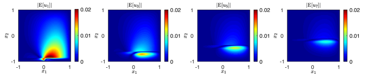
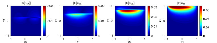
Figure 5: Absolute values of the means of the first order ANOVA expansion terms $|\mathrm{E}[u_{j}(x,\xi_{j})]|$ for $\nu=1/2$ on $1\times 16$ partition. The ANOVA terms with $\xi_{j}$ attached close to the top and bottom discontinuity have large values.

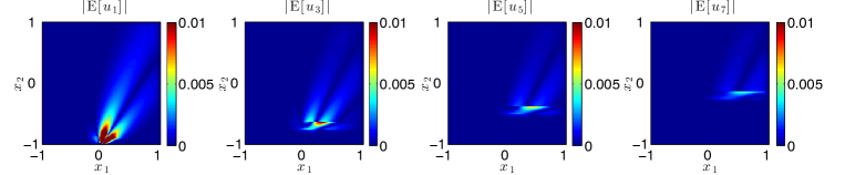
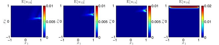
Figure 6: Absolute values of the means of the first order ANOVA expansion terms $|\mathrm{E}[u_{j}(x,\xi_{j})]|$ for $\nu=1/20$ on $1\times 16$ partition. The effect of the noise from each subdomain is more localized than the case of $\nu=1/2$.

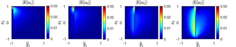
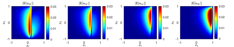
Figure 7: Absolute values of the means of the first order ANOVA expansion terms $|\mathrm{E}[u_{j}(x,\xi_{j})]|$ for $\nu=1/2$ on $16\times 1$ partition. The magnitudes of the ANOVA terms are less anisotropic than the case of $1\times 16$ since all of the directions are attached to the top discontinuity.

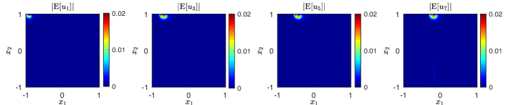
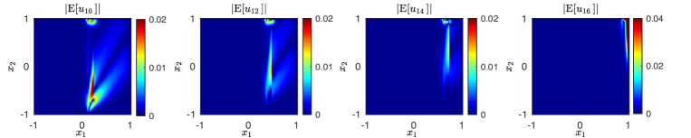
Figure 8: Absolute values of the means of the first order ANOVA expansion terms $|\mathrm{E}[u_{j}(x,\xi_{j})]|$ for $\nu=1/20$ on $16\times 1$ partition. The effect of the noise from each subdomain is more localized close to the top and bottom discontinuity than the case of $\nu=1/2$.

We first present the results where the ANOVA decomposition helps us to understand the impact of anisotropy on features of the solution. We use the reduced basis tolerance $\epsilon_{RB}=10^{-4}$ (see Algorithm 1) and the full ANOVA decomposition of the solution without truncation by setting $\epsilon_{A}=10^{-15}$ ( see (19)). Figure 4 plots magnitudes of the means of the first and second-order ANOVA terms, $\|\mathrm{E}[u_{j}(x,\xi_{j})]\|$ and $\|\mathrm{E}[u_{jk}(x,\xi_{j},\xi_{k})]\|$, for a $1\times 16$ partition (see Figure 1). The image on the left shows that the ANOVA terms for components of $\xi_{j}$ near the top boundary (large $j$), where there is a boundary layer, and near the bottom (small $j$), where there is a discontinuity along the inflow boundary, are large. Among the second order terms, the pairs involving the aforementioned directions and the terms with physically adjacent subdomains, e.g, $u_{j,j+1}(x,\xi_{j},\xi_{j+1})$, have large magnitudes as well. These points are further substantiated in Figure 5, where the absolute values of the means $|\mathrm{E}[u_{j}(x,\xi_{j})]|$ are plotted for several $j$. In particular, there is significant activity near discontinuities, $u_{16}$, $u_{14}$, and $u_{1}$. This is also true in the case of smaller diffusion parameter $\nu=1/20$ plotted in Figure 6. In addition, the system is more anisotropic compared to $\nu=1/2$ and the contribution is more localized in each subdomain. We emphasize that this feature will make the reduced basis algorithm based on ANOVA more efficient, since the existence of relatively important parameters indicates a possible truncation in the ANOVA decomposition. In constrast, Figures 7 and 8 show results for a $16\times 1$ partition. The maximum values of the ANOVA terms are all of the same order, in other words, the system is less anisotropic with respect to the parameters than the case of $1\times 16$, since all subdomains are attached to the top boundary layer. This is more apparent when $\nu=1/20$ in Figure 8, where the effect of the noise from each subdomain is more localized.

      $1\times 16$                                     $16\times 1$

mean

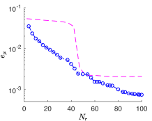
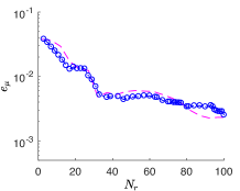
s.d.

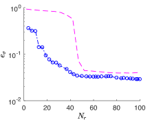
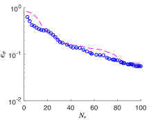
Figure 9: Error in the mean and standard deviation of the solution computed using reduced basis of size $N_{r}$. Shown results compare the reduced basis algorithm with and without the dimension-adaptive procedure for the problems on $1\times 16$ and $16\times 1$ partitions. The dimension-adaptive procedure using ANOVA decomposition has an advantage for anisotropic problems, e.g., $1\times 16$.

Next, we examine the quality of the reduced basis sorted using the ANOVA indicator $\gamma_{K}$ (13) as in Algorithm 2. Figure 9 plots the relative $L_{2}$-error in the moments with respect to the size of the reduced basis $N_{r}$ for the problems on $1\times 16$ and $16\times 1$ partitions with $\nu=1/2$. The errors are computed every two indices up to 100. The pink dashed lines show the error using the sparse-grid points of level two without the dimension-adaptive procedure, typically, generated in increasing order of index, e.g., $\xi_{1}$, $\xi_{2}$, $\cdots$, and $\xi_{12}$, $\xi_{13}$, $\cdots$. The initial saturation of the error in the $1\times 16$ case is due to this ordering, and the error drops suddenly after obtaining the reduced basis that has a large contribution to the solution, for instance, when the points using index $\xi_{16}$ are considered. However, our algorithm sorts the solution by the magnitude of $\gamma_{K}$ and the error effectively decays while avoiding an additional computation induced either by adopting the greedy procedure or sorting the reduced basis afterwards. This computation becomes particularly expensive for large $M$ and $N_{r}$, which makes our algorithm more preferable. This advantage is not apparent in the $16\times 1$ case shown in the second column, due to the fact that all directions are influenced in essentially the same way by the top boundary layer. However, our approach will show its effectiveness once the random variables $\{\xi_{j}\}$ have distinctive distributions.

Table 1: Number of full solves $N_{r}$ in the reduced basis collocation method using PCM-ANOVA points for $1\times 4$ partition and $\nu=1/20$.

$\ell$	$\ell=3$					1	2	3	4
$p$	3	5	7	9	11	$p=9$
$\epsilon_{RB}=10^{-3}$	3	4	4	4	4	4	4	4	4
$\epsilon_{RB}=10^{-4}$	16	24	31	35	37	15	25	35	38
$\epsilon_{RB}=10^{-5}$	33	63	80	90	97	25	74	90	103

$\ell=3$                                          $p=9$                    

mean

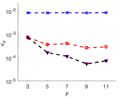
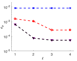
Figure 10: Relative $L_{2}$-error of the mean using the PCM-ANOVA collocation points with level $\ell$ and $p$ and reduced basis tolerance $\epsilon_{RB}$, for $1\times 4$ partition and $\nu=1/20$.

We close this section by presenting a convergence study of the PCM-ANOVA points in Figure 10 and Table 1, which motivates the necessity of adapting the resolution in each direction. Unlike the sparse-grid points, the ANOVA points have another independent parameter, the polynomial order $p$, in addition to the level $\ell$. Figure 10 shows the relative $L_{2}$-error of the mean with respect to these two parameters for a $1\times 4$ partition and $\nu=1/20$. The results are computed by either fixing the level $\ell=3$ or the polynomial order $p=9$. Although in both cases, the errors decrease with respect to $p$ and $\ell$, they tend to stagnate after certain maximal values are reached. Thus, the polynomial order and the level should be increased together with a carefully selected tolerance regarding the system [13].

3 Adaptive algorithm for RBM-ANOVA

In this section, we introduce an adaptive reduced basis algorithm by increasing the number of collocation points used to compute each ANOVA term, in other words, the polynomial order $p$ in each effective dimension $\mathcal{J}_{\ell}$ (19). As shown in Figure 10 and also later in Figure 11, fixed $p$ may limit accuracy. However, it is not practical to choose large $p$ from the beginning, since that leads to a large number of collocation points. Thus, we propose an adaptive PCM-ANOVA reduced basis algorithm that increases $p$ only among the active dimensions $\mathcal{J}_{\ell}$ and with an appropriate criterion that limits the increases in $p$.

The idea is shown in Algorithm 3. The method initializes the collocation points with polynomial order $p_{0}$, typically $p_{0}=3$, and level $\ell_{0}$. This choice will make the cost in the initial step to be smaller than that using a sparse-grid with the same level $\ell_{0}$. Then, among the effective dimensions $\mathcal{J}$ computed by the adaptive ANOVA criterion $\gamma_{K}$ (13), we increase $p$ in specific directions until a termination criterion holds. For this, we use a saturation condition that measures the relative difference of ANOVA terms in direction $K$ after increasing the polynomial order, that is,

$$\rho_{K}^{p_{K}}\doteq\frac{\|\mathrm{E}[{u}_{K}^{\bar{p}_{K}}]-\mathrm{E}[{u}_{K}^{p_{K}}]\|}{\|\sum_{|S|\leq|K|}\mathrm{E}[{u}_{S}]\|}<\epsilon_{p},$$ (21)

where ${u}_{K}^{p_{K}}$ is the ANOVA term in direction $K$ computed with the increased polynomial order $p_{K}$, and ${u}_{K}^{\bar{p}_{K}}$ is from the previous iteration, with $\bar{p}_{K}<{p}_{K}$. If this quantity is smaller than a prescribed tolerance $\epsilon_{p}=O(\epsilon_{RB})$, the reduced basis solution added in the current iteration is excluded from $\mathbf{S}_{N_{r}}$ and the direction $K$ is excluded from the set of effective dimensions $\mathcal{J}$. This condition is based on the error estimate of the stochastic spectral solution between large polynomial orders [38]. In addition, if all the error indicators (17) computed from the collocation points in the direction $K$ are less than the reduced basis tolerance $\epsilon_{RB}$, we exclude $K$ from $\mathcal{J}$. A stronger terminating criterion can be imposed by restricting the maximum order of polynomial at level $K$, $|K|=l$, from the previous level as $p_{K}\leq\max_{|S|=l-1}p_{S}$.

   1: Compute the solution $\mathbf{u}_{\xi^{(0)}}$ at the anchor point $\xi^{0}\in{\Xi_{0}}$.

   2: Initialize $\mathbf{S}_{\Theta_{r}}=\mathbf{u}_{\xi^{(0)}}$ and $\mathbf{Q}=\mathbf{u}_{\xi^{(0)}}/\|\mathbf{u}_{\xi^{(0)}}\|^{2}$ and construct the offline reduced matrices and vectors.

   3: Initialize active dimensions $\mathcal{J}=\cup_{l=1}^{\ell_{0}}\mathcal{J}_{l}$, $\mathcal{J}_{l}=\{K\subset\{1,...,M\}\,|\,|K|=l\}$, and $p_{K}=p_{0}$ for all $K\in\mathcal{J}$.

   4: for   $\ell_{0}\leq l\leq\ell$ do

   5:     while   $\mathcal{J}\neq\emptyset$ do

   6:        Store $\bar{\mathcal{J}}=\mathcal{J}$.

   7:        for $K\in\mathcal{J}$ do

   8:           Store $\bar{{u}}={u}_{K}$ and $\bar{\mathbf{Q}}=\mathbf{Q}$.

   9:           Update $\mathbf{Q}$ in direction $K$, $(\mathbf{Q},\mathbf{S}_{K})$ = RBM($\mathbf{Q}$, $\Xi_{K}^{p_{K}}$, $\epsilon_{RB}$) in Algorithm 1.

10:           Compute the ANOVA term ${u}_{K}$ and indicator $\gamma_{K}$ in (13).

11:           if $\mathbf{Q}=\bar{\mathbf{Q}}$ or $\gamma_{K}<\epsilon_{A}$ or $\rho_{K}^{p_{K}}<\epsilon_{p}$ in (21) then

12:              Exclude term $K$, i.e., $\mathcal{J}=\mathcal{J}\setminus K$, and reset ${u}_{K}=\bar{{u}}$, $\mathbf{Q}=\bar{\mathbf{Q}}$.

13:           else

14:              Increase polynomial order $p_{K}$.

15:           end

16:        end

17:        Update $\mathbf{S}_{\Theta_{r}}=[\mathbf{S}_{\Theta_{r}},\mathbf{S}]$, where $(\mathbf{S},\mathcal{J}_{l})$ = RB-Sort($\{\gamma_{K}\}_{K\in\bar{\mathcal{J}}}$, $\{\mathbf{S}_{K}\}_{K\in\bar{\mathcal{J}}}$, $\bar{\mathcal{J}}$) in Algorithm 2.

18:     end

19:     Select active dimensions $\widetilde{\mathcal{J}}_{l}=\{K\in\mathcal{J}_{l}\,|\,|K|=l,\,\gamma_{K}>\epsilon_{A}\}$.

20:     Set next level indices $\mathcal{J}_{l+1}=\{|K|=l+1\,|\,K=\cup_{T\in\widetilde{\mathcal{J}}_{l}}T\}$ and $\mathcal{J}=\mathcal{J}_{l+1}$.

21: end

Algorithm 3 Adaptive-RBM PCM-ANOVA( $\{\Xi_{l}^{p}\}_{l=0}^{\ell}$, $\epsilon_{RB}$, $\epsilon_{A}$, $\epsilon_{p}$ ) : Reduced basis method based on dimension and $p$-adaptive PCM-ANOVA collocation points up to level ${\ell}$. The parameters are typically chosen as $\ell_{0}=1$ or $2$ and $p_{0}=3$.

3.1 Numerical results

$1\times 16$                              $\qquad 4\times 4$                              $\qquad 16\times 1$

mean

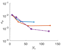
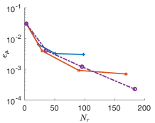
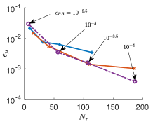
s.d.

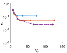
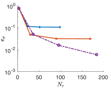
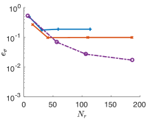
Figure 11: Error in the mean and standard deviation versus the size of reduced basis $N_{r}$ for the case of diffusion parameter $\nu=1/2$ and $N_{D}=16$. The solution is computed by RBM using PCM-ANOVA with fixed $p$ or an adaptive $p$ with $\epsilon_{p}=10^{-5}$. The bullets correspond to varying $\epsilon_{RB}$ from $10^{-2.5}$ to $10^{-4}$.

$1\times 16$                              $\qquad 4\times 4$                              $\qquad 16\times 1$

mean

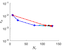
s.d.

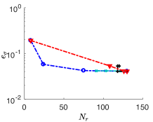
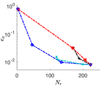
Figure 12: Error in the mean and standard deviation versus the size of reduced basis $N_{r}$ for the case of diffusion parameter $\nu=1/2$ and $N_{D}=16$. The bullets correspond to solutions computed by varying each tolerance $\epsilon_{RB}$, $\epsilon_{A}$, and $\epsilon_{p}$ from $10^{-2.5}$ to $10^{-4}$, while others are fixed as $10^{-4}$. The results for $\epsilon_{RB}=\epsilon_{A}=\epsilon_{p}$ are shown as well. The reduced basis solution is more accurate when $\epsilon_{A},\epsilon_{p}<\epsilon_{RB}$.

We first study the adaptive strategies in Algorithm 3 for benchmark problems on $N_{D}=16$ subdomains with $1\times 16$, $4\times 4$, and $16\times 1$ partitions. The initial parameters are selected as $p_{0}=3$ and $\ell_{0}=2$, and we successively increase $p_{K}$ by 2. We have three different tolerances to investigate, the reduced basis acceptance $\epsilon_{RB}$, the truncation of the ANOVA decomposition $\epsilon_{A}$, and the polynomial order $\epsilon_{p}$.

We first point out in Figure 11 the advantage of adapting the polynomial order $p$. The tolerance $\epsilon_{RB}$ varies from $10^{-2.5}$ to $10^{-4}$, while $\epsilon_{p}=10^{-5}$, and $\epsilon_{A}=10^{-15}$ to prevent ANOVA truncation. The error of the reduced basis solution computed with fixed polynomial orders $p=3$ or $5$ does not decay after reaching a certain level. The accuracy is not improved while the size of the reduced basis increases. The adaptive procedure for $p$ overcomes this problem.

Next, we study the sensitivity of the method with respect to the tolerance. One of the tolerances among $\epsilon_{RB}$, $\epsilon_{A}$, and $\epsilon_{p}$ is varied from $10^{-2.5}$ to $10^{-4}$, while others are fixed as $10^{-4}$. We also test the case where all the tolerances are reduced simultaneously as $\epsilon_{RB}=\epsilon_{A}=\epsilon_{p}$. The results are plotted in Figure 12 which shows that all the errors eventually converge to the level attained by $\epsilon_{RB}=\epsilon_{A}=\epsilon_{p}=10^{-4}$. Moreover, the selected reduced basis solution is more accurate when $\epsilon_{p}$ is less than $\epsilon_{RB}$. In further simulations, we take $\epsilon_{p}=\epsilon_{RB}/C$, for some constant $C$, e.g., $C=2$. On the other hand, results for $\epsilon_{A}<10^{-3.5}$ show no difference since the effective dimensions $\mathcal{J}_{\ell}$ include all directions (see Figure 4 for the magnitude of the ANOVA terms in the $1\times 16$ case). Thus, $\epsilon_{A}$ should be chosen carefully by taking into consideration the trend of $\gamma_{K}$ to balance accuracy and computational complexity.

$\|\mathrm{E}[u_{j}]\|$                                  $p_{j}$                                  $N_{r_{j}}$

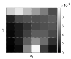
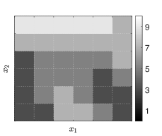
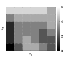
Figure 13: The mean of the first order ANOVA expansion term $\|\mathrm{E}[u_{j}]\|$, the maximum polynomial order $p_{j}$, and the number of points selected as the reduced basis $N_{r_{j}}$ on each subdomain $D_{j}$ with $\xi_{j}$ parameter for $6\times 6$ and $\nu=1/2$. The importance of the subdomains near the top boundary layer and the bottom inflow discontinuity is automatically identified by the algorithm, as is evident in all three figures.

We now investigate the performance of our algorithm in higher dimensional parametric space, considering $6\times 6$, $8\times 8$, and $10\times 10$ subdomain partitions. The reduced basis tolerance $\epsilon_{RB}$ is varied from $10^{-2.5}$ to $10^{-4}$, and $\epsilon_{A}$ and $\epsilon_{p}$ are taken to be proportional to $\epsilon_{RB}$, $\epsilon_{A}=\epsilon_{p}=\epsilon_{RB}/2$. In Figure 13 shows the solution on a $6\times 6$ partition with diffusion parameter $\nu=1/2$ using tolerance $\epsilon_{RB}=10^{-4}$. On each subdomain $D_{j}$ with parameter $\xi_{j}$, the figures plot the magnitude of the first order ANOVA terms $\|\mathrm{E}[u_{j}]\|$, the adapted maximum polynomial order $p_{j}$ in direction $j$, and the number of reduced basis $N_{r_{j}}$ selected in direction $j$. They show that the algorithm automatically increases the polynomial order and selects more reduced basis solutions on the subdomains near the top boundary layer and the bottom inflow discontinuity, where the ANOVA term is relatively large.

Let us compare the efficiency of the reduced basis algorithm using a fixed polynomial order $p=9$ and adaptive determination of $p$. Table 2 shows the reduced basis size and the error in the moments for diffusion parameter $\nu=1/20$ (top) and $\nu=1/2$ (bottom). With a slightly smaller value of $\epsilon_{RB}$, the adaptive $p$ approach yields a reduced basis set that achieves the same level of accuracy with the fixed $p$ approach. Figure 14 shows accuracy versus computational time for both fixed $p$ and adaptively determined $p$ (These results were obtained in Matlab 2016 on a 3.33GHz Intel core i5 processor). It can be seen that changing $p$ adaptively significantly reduces the computational cost. The computational cost saving of the adaptive $p$ approach is primarily due to its use of fewer search points $C(M,\ell)$ in (18), as shown in Table 3. We compare the total number of points on which the reduced basis is searched between using the PCM-ANOVA collocation points in the entire $M$-dimensions with a fixed $p=9$, adapting directions with a fixed $p=9$, and adapting both directions and $p$. Compared to considering a tensor product, which yields $p^{M}$ points, the number of PCM-ANOVA points $C(M,\ell)$ is reduced by the truncation in the interaction level with $\ell=2$. However, the number is large due to the high dimensionality of size $M$, and the adaptive approach in both dimension and $p$ reduces the computational cost. For the case of $\nu=1/20$, due to its strong anisotropy, the cost saving is significant. When $\nu=1/2$, although the cost saving from the truncation of directions is less than for $\nu=1/20$, the procedure of adaptive $p$ reduces the cost further by increasing $p$ only among the effective dimensions.

Table 2: The size of reduced basis $N_{r}$ and the error in the moments $e_{\mu}$ and $e_{\sigma}$ for $N_{D}\times N_{D}$ partitions and diffusion parameter $\nu=1/2$ (top) and $\nu=1/20$ (bottom), comparing the reduced basis algorithm with adaptive $p$ and fixed $p=9$. Corresponding computational time is plotted in Figure 14.

$\nu=1/2$		adapt $p$			fixed $p=9$
$\epsilon_{RB}$		$10^{-2.5}$	$10^{-3}$	$10^{-3.5}$	$10^{-2.5}$	$10^{-2.9}$	$10^{-3.4}$
$6\times 6\,\,\,$	$N_{r}$	3	34	157	3	38	191
	$e_{\mu}$	3.156e-02	1.067e-02	2.756e-03	3.507e-02	1.391e-02	2.700e-03
	$e_{\sigma}$	7.634e-01	2.632e-01	5.282e-02	7.244e-01	2.785e-01	5.440e-02
$8\times 8\,\,$	$N_{r}$	3	26	197	3	37	291
	$e_{\mu}$	3.381e-02	2.234e-02	1.474e-03	3.626e-02	1.980e-02	1.377e-03
	$e_{\sigma}$	7.767e-01	5.135e-01	5.480e-02	7.411e-01	3.996e-01	5.487e-02
$10\times 10\,$	$N_{r}$	3	35	248	3	43	385
	$e_{\mu}$	3.578e-02	2.411e-02	1.793e-03	3.751e-02	2.239e-02	1.680e-03
	$e_{\sigma}$	7.858e-01	4.973e-01	6.340e-02	7.533e-01	4.140e-01	6.272e-02

$\nu=1/20$		adapt $p$			fixed $p=9$
$\epsilon_{RB}$		$10^{-3}$	$10^{-3.5}$	$10^{-4}$	$10^{-3}$	$10^{-3.4}$	$10^{-3.9}$
$6\times 6\,\,\,$	$N_{r}$	13	24	85	13	29	89
	$e_{\mu}$	8.095e-03	4.415e-03	1.073e-03	8.749e-03	4.897e-03	1.086e-03
	$e_{\sigma}$	6.279e-01	2.424e-01	2.305e-02	6.335e-01	2.448e-01	2.515e-02
$8\times 8\,\,$	$N_{r}$	15	30	118	17	31	119
	$e_{\mu}$	9.287e-03	5.736e-03	1.242e-03	8.942e-03	5.899e-03	1.348e-03
	$e_{\sigma}$	6.777e-01	2.670e-01	3.429e-02	6.195e-01	2.676e-01	3.582e-02
$10\times 10\,$	$N_{r}$	16	34	137	21	35	153
	$e_{\mu}$	9.159e-03	5.574e-03	9.333e-04	8.447e-03	6.093e-03	9.052e-04
	$e_{\sigma}$	7.037e-01	3.208e-01	2.363e-02	6.196e-01	3.237e-01	2.448e-02

         $6\times 6$                                     $8\times 8$                                     $10\times 10$

$\nu=1/2$

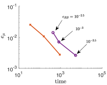
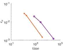
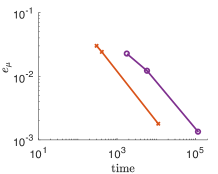
$\nu=1/20$

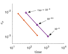
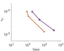
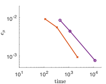
Figure 14: Error in the mean and standard deviation versus computational time in seconds. The solution is computed with fixed $p=9$ and adaptive $p$ with $\epsilon_{RB}=10^{-3}$ to $10^{-4}$.

Table 3: Comparison of the number of search points $C(M,\ell)$ (12) using the entire directions in $M$ dimensions with a fixed polynomial order $p=9$, adapting direction with a fixed $p=9$, and adapting both direction and $p$.

		$8\times 8$			$10\times 10$
$\nu$	$\epsilon_{RB}$	$M=64$	adapt $M$		$M=100$	adapt $M$
		$p=9$	$p=9$	adapt $p$	$p=9$	$p=9$	adapt $p$
1/2	$10^{-3}$	$\begin{matrix}C(64,2)\\ =129536\end{matrix}$	24704	542	$\begin{matrix}C(100,2)\\ =317600\end{matrix}$	38880	512
1/2	$10^{-3.5}$		99072	13924		223904	25410
1/20	$10^{-3}$		2304	122		3680	156
1/20	$10^{-3.5}$		6336	246		10592	288

4 Conclusion

In this paper, we developed an adaptive reduced basis method for anisotropic parametrized stochastic PDEs based on the PCM and ANOVA approximation. The proposed algorithm enhances the reduced basis collocation methods by first obtaining the effective dimensions and then increasing the resolution in those directions. The dimensional adaptive procedure based on the ANOVA decomposition reduces the computational cost significantly for an anisotropic problem. In addition, the ANOVA indicator rearranges both of the search directions and the reduced basis solution, so that the reduced basis is sorted in a descending order of error with lower computational cost than the cost that typically occurs in greedy type approaches. The second adaptive procedure increases the resolution in each direction among the effective dimensions. This eliminates the stagnation of the error that may occur by fixing the polynomial order in PCM. Moreover, this adaptive procedure can be terminated when the ANOVA term converges. The proposed adaptive reduced basis algorithm is implemented on the stationary stochastic convection-diffusion problem. The algorithm effectively detects the directions in the stochastic space that are associated with the irregularity of the solution, for instance, discontinuous boundary conditions and steep boundary layers. By emphasizing those directions and by increasing the number of collocation points until necessary, the algorithm reduces the computational cost while improving accuracy in the moments.

Our future work includes analysis of the proposed adaptive reduced basis algorithm using reduced basis error indicators based on posterior error estimates of parametrized PDEs [27] and combining them with analytical studies of adaptive PCM [38, 14] and anchored ANOVA method [44]. In addition, we aim to further investigate the effect of the quadrature rules, e.g., Clenshaw-Curtis and Gauss abscissae, as candidate points to the accuracy of the reduced basis solution. Since different choice for the interpolation and anchor points in PCM-ANOVA yields significantly distinct set of collocation points, strategies to utilize the error estimates involving different interpolation points [37, 25] and to choose the anchor point that minimizes the error estimates of the ANOVA approximation [43, 44] may be useful. Finally, extending our algorithm to nonlinear and time-dependent problems, for example, stochastic Navier-Stokes equation, is another future direction. Various techniques including linearized iterative solvers such as Newton iterations [17, 12] and empirical interpolation methods [2, 9] can be employed.

- [1] Babuska, I., Nobile, F., and Tempone, R. A stochastic collocation method for elliptic partial differential equations with random input data. SIAM J. Numer. Analysis 45, 3 (2007), 1005–1034.
- [2] Barrault, M., Maday, Y., Nguyen, N. C., and Patera, A. T. An ‘empirical interpolation’ method: application to efficient reduced-basis discretization of partial differential equations. C. R. Math. Acad. Sci. 339 (2004), 667–672.
- [3] Barthelmann, V., Novak, E., and Ritter, K. High dimensional polynomial interpolation on sparse grids. Adv. Comput. Math. 12 (2000), 273–288.
- [4] Braess, D. Finite Elements, third ed. Cambridge University Press, London, 2007.
- [5] Cao, Y., Chen, Z., and Gunzbuger, M. ANOVA expansions and efficient sampling methods for parameter dependent nonlinear PDEs. Int. J. Numer. Anal. Model. 6 (2009), 256–273.
- [6] Chen, P., and Quarteroni, A. Weighted reduced basis method for stochastic optimal control problems with elliptic PDE constraint. SIAM/ASA J. Uncertainty Quantification 2 (2014), 364–396.
- [7] Chen, P., and Quarteroni, A. A new algorithm for high-dimensional uncertainty quantification based on dimension-adaptive sparse grid approximation and reduced basis methods. J. Comp. Phys. 298 (2015), 176–193.
- [8] Chen, P., Quarteroni, A., and Rozza, G. Comparison between reduced basis and stochastic collocation methods for elliptic problems. J. Sci. Comput. 59 (2014), 187–216.
- [9] Elman, H. C., and Forstall, V. Numerical solution of the steady-state Navier-Stokes equations using empirical interpolation methods. Computer Methods in Applied Mechanics and Engineering 317 (2017), 380–399.
- [10] Elman, H. C., and Liao, Q. Reduced basis collocation methods for partial differential equations with random coefficients. SIAM/ASA J. Uncertainty Quantification 1 (2013), 192–217.
- [11] Elman, H. C., Ramage, A., and Silvester, D. J. Algorithm 886: IFISS, a Matlab toolbox for modelling incompressible flow. ACM Trans. Math. Software 33 (2007).
- [12] Elman, H. C., Silvester, D. J., and Wathen, A. J. Finite Elements and Fast Iterative Solvers, second ed. Oxford University Press, 2014.
- [13] Foo, J., and Karniadakis, G. E. Multi-element probabilistic collocation method in high dimensions. J. Comp. Phys. 229 (2010), 1536–1557.
- [14] Foo, J., Wan, X., and Karniadakis, G. E. The multi-element probabilistic collocation method (ME-PCM): Error analysis and applications. J. Comp. Phys. 227 (2008), 9572–9595.
- [15] Ghanem, R. G., and Spanos, P. D. Stochastic Finite Elements: A Spectral Approach. Springer-Verlag, 1998.
- [16] Griebel, M. Sparse grids and related approximation schemes for higher dimensional problems. In Foundations of Computational Mathematics, Santander 2005 (2006), L. M. Pardo, A. Pinkus, E. Süli, and M. J. Todd, Eds., no. 331, Cambridge University Press, pp. 106–161.
- [17] Gunzburger, M., Peterson, J., and Shadid, J. Reduced-order modeling of time-dependent PDEs with multiple parameters in the boundary data. Comput. Methods Appl. Mech. Engrg. 196 (2007), 1030–1047.
- [18] Hesthaven, J. S., and Zhang, S. On the use of anova expansions in reduced basis methods for high-dimensional parametric partial differential equation. J. Sci. Comp. 69 (2016), 292–313.
- [19] Ito, K., and Ravindran, S. S. A reduced-order method for simulation and control of fluid flows. J. Comp. Phys. 143, 2 (1998), 403–425.
- [20] Liao, Q., and Lin, G. Reduced basis anova methods for partial differential equations with high-dimensional random inputs. J. Comp. Phys. 317 (2016), 148–164.
- [21] Løvgren, A. E., Maday, Y., and Rønquist, E. M. A reduced basis element method for the steady stokes problem : application to hierarchical flow systems. Model. Identif. Control 27 (2006), 79–94.
- [22] Ma, X., and Zabaras, N. An adaptive hierarchical sparse grid collocation method for the solution of stochastic differential equations. J. Comp. Phys. 228 (2009), 3084–3113.
- [23] Ma, X., and Zabaras, N. An adaptive high dimensional stochastic model representation technique for the solution of stochastic partial differential equations. J. Comp. Phys. 299 (2010), 3884–3915.
- [24] Nobile, F., Tempone, R., and Webster, C. A sparse grid stochastic collocation method for partial differential equations with random input data. SIAM J. Numer. Analysis 46, 5 (2008), 2309–2345.
- [25] Novelinkovà, M. Comparison of Clenshaw-Curtis and Gauss quadrature. In WDS’11 Proceedings of Contributed Papers: Part I (2011), pp. 67–71.
- [26] Papoulis, A. Probability, Random Variables and Stochastic Processes, third ed. McGraw-Hill, 1991.
- [27] Patera, A. T., and Rozza, G. Reduced Basis Approximation and A Posteriori Error Estimation for Parametrized Partial Differential Equations, first ed. MIT Pappalardo Graduate Monographs in Mechanical Engineering, 2006.
- [28] Peterson, J. The reduced basis method for incompressible viscous flow calculations. SIAM J. Sci. Stat. Comput. 10 (1989), 777–786.
- [29] Porsching, T. A., and Lee, M. L. The reduced basis method for initial value problems. SIAM J. Numer. Anal. 24 (1987), 1277–1287.
- [30] Prud’homme, C., Rovas, D. V., Veroy, K., Machiels, L., Maday, Y., Patera, A. T., and Turinici, G. Reliable real-time solution of parametrized partial differential equations: Reduced-basis output bound methods. J. Fluids Eng 124 (2001), 70–80.
- [31] Quarteroni, A., Manzoni, A., and Negri, F. Reduced Basis Methods for Partial Differential Equations, first ed. Springer International Publishing, 2016.
- [32] Quarteroni, A., Rozza, G., and Manzoni, A. Certified reduced basis approximation for parametrized partial differential equations and applications. J. Math. Indust. 1 (2011), 1–49.
- [33] Rozza, G., Huynh, D. B. P., and Patera, A. T. Reduced basis approximation and a posteriori error estimation for affinely parametrized elliptic coercive partial differential equations. Archives of Computational Methods in Engineering 15 (2008), 229–275.
- [34] Schwab, C., and Suli, E. Adaptive galerkin approximation algorithms for partial differential equations in infinite dimensions. Tech. report, Seminar for Applied Mathematics, ETH 11, 69 (2012), 1–25.
- [35] Silvester, D. J., Elman, H. C., and Ramage, A. Incompressible flow and iterative solver software (IFISS 3.5). \urlhttps://www.cs.umd.edu/users/elman/ifiss3.5.html, 2016.
- [36] Todor, R. A., and Schwab, C. Convergence rates for sparse chaos approximations of elliptic problems with stochastic coefficients. IMA J. Numer. Anal. 27 (2007), 232–261.
- [37] Trefethen, L. N. Is Gauss quadrature better than Clenshaw Curtis? SIAM Review 50 (2008), 67–87.
- [38] Wan, X., and Karniadakis, G. E. An adaptive multi-element generalized polynomial chaos method for stochastic differential equations. J. Comp. Phys. 209, 2 (2005), 617–642.
- [39] Xiu, D., and Hesthaven, J. High-order collocation methods for differential equations with random inputs. SIAM J. Sci. Comput. 27, 3 (2005), 1118–1139.
- [40] Xiu, D., and Karniadakis, G. E. The Wiener-Askey polynomial chaos for stochastic differential equations. SIAM J. Sci. Comput. 24, 2 (2002), 619–644.
- [41] Xiu, D., and Karniadakis, G. E. Modeling uncertainty in flow simulations via generalized polynomial chaos. J. Comp. Phys. 187 (2003), 137–167.
- [42] Yang, X., Choi, M., and Karniadakis, G. E. Adaptive ANOVA decomposition of stochastic incompressible and compressible fluid flows. J. Comp. Phys. 231 (2012), 1587–1614.
- [43] Zhang, Z., Choi, M., and Karniadakis, G. E. Anchor points matter in ANOVA decomposition. Proceedings of ICOSAHOM’09, Springer, eds. E. Ronquist and J. Hesthaven (2010).
- [44] Zhang, Z., Choi, M., and Karniadakis, G. E. Error estimates for the ANOVA method with polynomial chaos interpolation: Tensor product functions. SIAM J. Sci. Comp. 34, 2 (2012), 1165–1186.