Solvable two-dimensional superconductors with $l$-wave pairing

Abstract

We analyze a family of two-dimensional BCS Hamiltonians with general $l$-wave pairing interactions, classifying the models in this family that are Bethe-ansatz solvable in the finite-size regime. We show that these solutions are characterized by nontrivial winding numbers, associated with topological phases, in some part of the corresponding phase diagrams. By means of a comparative study, we demonstrate benefits and limitations of the mean-field approximation, which is the standard approach in the limit of a large number of particles. The mean-field analysis also allows to extend part of the results beyond integrability, clarifying the peculiarities associable with the integrability itself.

I Introduction

Superconductivity, a phenomenon that is typical in condensed matter physics, but also relevant in nuclear and subnuclear physics (see, for instance, alford2008 ; anglani2014 ), takes its origin from pairing between fermions. It is typically described assuming an interacting (pairing) Hamiltonian and solving it via the mean-field (MF) approximation BCS57 , which explicitly violates particle number conservation. While this limitation has a small effect on macroscopic systems, it can lead to dramatic deviations when fluctuations are important, i.e. when dealing with a fixed small number of particles. This justifies the interest in the study of exactly solvable models that avoid any approximation, at the price of assuming specific forms of the interactions, like in the so-called Richardson model Richardson63 with $s$-wave pairing ($l=0$). This model is known to be integrable and its exact solution is known to be related to the Gaudin spin Hamiltonians ref1 ; ref2 . This exact-solution approach allowed various generalizations of the Richardson-Gaudin models germanrev ; sierralungo ; ortiz2014 , relevant for condensed matter and nuclear physics. In general, Richardson-Gaudin particle-conserving integrable models can be classified into rational, hyperbolic, and trigonometric classes. Within this classification, a realization of the hyperbolic model is the $p_{x}+ip_{y}$ model, which has been extensively studied ref4 ; sierra09 ; VanRaemdonck2014 ; ortiz2005 ; ortiz2010 ; dukelsky2011 ; pan1998 , also in the presence of interfaces with normal conductors (see e.g. fisher2012 ; giuliano2013 ; affleck2014 ).

These examples motivate the need for analyzing integrable models for superconductivity, by elucidating the physics of some delicate aspects of strongly correlated quantum systems (see also recati ). Particularly intriguing is the possibility to include pairing interactions with higher angular momentum (a pivotal example being the $d$-wave, i.e. $l=2$, even chiral) in two-dimensional (2D) systems, due to their direct implication for high-temperature superconductivity leerev . Among the plethora of compounds and lattice schemes belonging to this family, we report the very recent realization of high-temperature (and likely $d$-wave) superconductivity on twisted bilayer graphene jarillo2018 . Still on the experimental side, the $p$-wave ($l=1$) pairing is present in ³He volovik and in strontium ruthenates mackanzie2003 ; maeno2012 , while $f$-wave pairing occurs for instance in superfluid ³He gould1986 ; halperin2006 . Moreover, new progress in the physics of ultracold Fermi gases opens up the possibility to design superconductive pairings up to the $h$-wave ($l=5$), see e.g. anna ; mathey2007 ; dutta2010 ; sarma2010 ; mao2011 ; hao2013 ; wu2013 ; bou2017 .

Motivated by these possibilities and by the considerable theoretical interest in the high-wave superconductivity, in the present paper we analyze a large family of 2D BCS models with arbitrary $l$-wave ($l_{x}+i\,l_{y}$) pairing interaction. A particular attention is posed on the phase content of these models. We first discuss (Sec. II) the cases that can be exactly solved via the Bethe-ansatz in a finite-size system. Later, we describe a standard MF analysis (Sec. III), and we compare the results from the two different approaches studying the topological properties of their solutions (Sec. IV). In this way, further insight is also achieved for the cases where integrability does not hold, as well as for the role of integrability itself.

The family of superconductive models that we are going to study is described by Hamiltonians of the form

$$H=\sum_{{\bf k}}\epsilon_{{\bf k}}c_{{\bf k}}^{\dagger}c_{{\bf k}}-g\sum_{{\bf kk}^{\prime}}(k_{x}-ik_{y})^{l}(k^{\prime}_{x}+ik^{\prime}_{y})^{l}c_{{\bf k}}^{\dagger}c_{-{\bf k}}^{\dagger}c_{-{\bf k}^{\prime}}c_{{\bf k}^{\prime}}\,.$$ (1)

There $c_{{\bf k}}^{\dagger}$ is the creation operators of 2D fermions with momentum ${\bf k}=(k_{x},k_{y})$, and $g$ is the coupling constant, positive for an attractive interaction. Notice that the interaction term creates and annihilates pairs of fermions with opposite momentum. In order to keep the widest generality, at the beginning of our analysis we do not adopt any particular choice for the single particle energy $\epsilon_{\mathbf{k}}$, only assuming it is a function of the modulus $k\equiv|\mathbf{k}|$.

In Eq. (1), we have dropped the spin index $\{\uparrow,\downarrow\}$ in the Fermi operators, so spinless fermions are formally considered. If instead the Cooper pairs are spinful, the symmetry of their spin wavefunctions is univocally determined by the Fermi-Dirac statistics. In fact, when $l$ is even, the Cooper pairs form a spin singlet (antisymmetric), while when $l$ is odd they are in the triplet sector (symmetric and polarized). In both the cases, the structure of the Bethe-ansatz equations and of the spatial part of the exact Cooper wavefunctions (introduced in Sect. II) in the presence of integrability are the same as in the spinless model described in Eq. (1).

The familiar $s$-wave case corresponds to $l=0$ and to the singlet sector of the spin wavefunction. This is the sole non symmetry-breaking case under parity and time reversal transformation. The breaking of these symmetries for $l\geq 1$ leads to different kinds of exact solutions, introducing nontrivial topological properties of the paired states (according to the ten-fold way classification for the topological insulators and superconductors, see e. g. zirnbauer1996 ; zirnbauer1997 ; ludwig2009 ; ludwig2010 ).

II Exact solution in the integrable cases

II.1 General setting

In the present Section we address the exact solution of the Hamiltonian in Eq. (1). We find that the precise forms of $\epsilon_{\mathbf{k}}$ and of the Cooper wavefunctions are constrained by requiring the integrability.

The first step to proceed on is to notice that when only a single fermion occupies the level in ${\bf k}$ or $-{\bf k}$ (i.e. without its partner), it decouples from the ground-state dynamics, due to the interaction in Eq. (1). So, it is convenient to restrict ourselves to the dynamics of the Cooper pairs, having creation operators $b_{{\bf k}}^{\dagger}=c_{{\bf k}}^{\dagger}c_{-{\bf k}}^{\dagger}$ (see e.g. germanrev ). Accordingly, the Hamiltonian in Eq. (1) takes the form

$$H=\sum_{{\bf k}}2\,\epsilon_{{\bf k}}\,b_{{\bf k}}^{\dagger}b_{{\bf k}}-g\,B_{0}^{\dagger}B_{0}\,.$$ (2)

Due to the particular factorized form of the interaction in Eq. (1), $H$ is now quadratic in terms of the new operator $B_{0}^{\dagger}=\sum_{{\bf k}}z_{{\bf k}}\,b_{{\bf k}}^{\dagger}$ where $z_{{\bf k}}=(k_{x}-ik_{y})^{l}$ are called pairing functions. Clearly, if the $b_{{\bf k}}$ operators were truly bosonic, the Hamiltonian would be directly diagonalizable. However, the $b_{{\bf k}}$ are instead hard-core bosons obeying the following commutation relations

$$\left[b_{{\bf k}},b_{{\bf k}^{\prime}}^{\dagger}\right]=\delta_{{\bf kk}^{\prime}}(1-2\,b_{{\bf k}}^{\dagger}b_{{\bf k}})\,.$$ (3)

As a trial wave function for $p$ pairs, we take the following general ansatz

$$|\Psi_{p}\rangle=\prod_{\nu=1}^{p}B_{J_{\nu}}^{\dagger}|0\rangle\,,\qquad B_{J}^{\dagger}=\sum_{{\bf k}}w_{{\bf k}}(J)\,b_{{\bf k}}^{\dagger}\,.$$ (4)

and we impose the eigenvalue equation

$$(H-\mathcal{E}_{p})|\Psi_{p}\rangle=0\,,$$ (5)

where the total energy $\mathcal{E}_{p}$ is given by the sum of the pair energies, $\mathcal{E}_{p}=\sum_{\nu=1}^{p}E_{J_{\nu}}$.

The next two sections will be devoted to the solution of Eq. (5) for one single pair and for multi-pair configurations. Generally, these solutions are obtained using the algebra of the pseudo-bosonic commutation relations to shift $H$ in Eq. (5) through the operators $B_{J_{\nu}}^{\dagger}$ contained in $|\Psi_{p}\rangle$, until $H$ acts on the vacuum $|0\rangle$, giving zero vondelft1999 . As the detailed calculation is rather cumbersome, it is presented in Appendix A.

II.2 One pair case

By restricting the eigenvalue equation in Eq. (5) to one pair $|\Psi_{1}\rangle$ with energy $E_{J}$, we obtain the condition:

$$w_{{\bf k}}(J)=g\frac{z_{{\bf k}}}{2\epsilon_{{\bf k}}-E_{J}}\sum_{{\bf k}^{\prime}}z_{{\bf k}^{\prime}}^{*}\,w_{{\bf k}^{\prime}}(J)\,.$$ (6)

Multiplying both sides by $z_{{\bf k}}^{*}$ and summing in ${\bf k}$ (which is customary for the gap equations in the BCS theory grosso ; annett ), unless the "order parameter" $W(J)=\sum_{{\bf k}}\,z_{{\bf k}}^{*}w_{{\bf k}}(J)$ is zero, we obtain the Richardson equation for one pair,

$$1-g\sum_{{\bf k}}\frac{|z_{{\bf k}}|^{2}}{2\epsilon_{{\bf k}}-E_{J}}=0\,,$$ (7)

as well as the expressions for the ansatz’s coefficients

$$w_{{\bf k}}(J)=gW(J)\,\frac{z_{{\bf k}}}{2\epsilon_{{\bf k}}-E_{J}}\,,$$ (8)

proportional to the wavefunction $\frac{z_{{\bf k}}}{2\epsilon_{{\bf k}}-E_{J}}$. The proportionality factors $g\,W(J)$ do not depend on ${\bf k}$, thus they are irrelevant and can be neglected, as they affect only normalizations and global phases. Consequently, without any loss of generality, we can retain the wave function

$$w_{{\bf k}}(J)=\frac{z_{{\bf k}}}{2\epsilon_{{\bf k}}-E_{J}}\,.$$ (9)

Notice that the spatial wavefunction (9) has the same parity of $l$ under the transformation $\bf{k}\to-\bf{k}$. This fact has a direct consequence on the symmetry of the spin part of the wavefunction, as discussed in the Introduction. Moreover, if two spins $\{\uparrow,\downarrow\}$ are involved in the Cooper pair, still at fixed $l$, the forms of the Hamiltonian in Eq. (2) and of the commutators in Eq. (3) (as well as of the consequent ones including the operators $B_{J}$, see the Appendix A) remain unchanged. Therefore, the structure of the Bethe-ansatz equations and of the spatial part of the exact Cooper wavefunctions also do not change.

II.3 Many pairs

Similar to the one-pair case in the previous subsection, the ansatz in Eq. (4) for the $p$ pair case reads

$$|\Psi_{p}\rangle=\prod_{\nu=1}^{p}B_{J_{\nu}}^{\dagger}|0\rangle\,,\qquad B_{J}^{\dagger}=\sum_{{\bf k}}\frac{z_{{\bf k}}}{2\epsilon_{{\bf k}}-E_{J}}b_{{\bf k}}^{\dagger}\,,$$ (10)

where we have assumed the expression in Eq. (9) for the wavefunctions. The solution of Eq. (5), discussed in detail in Appendix A, yields the following final equations analogous to Eq. (7). These solutions can be classified into three groups, depending on the form of $z_{{\bf k}}$:

1. The pairing function $z_{{\bf k}}$ is independent of $\mathbf{k}$. A relevant case is obtained by fixing $z_{{\bf k}}=1$; therefore, from Eq. (46), we get the well-known Richardson equations

   $$1-g\sum_{{\bf k}}\frac{1}{2\epsilon_{{\bf k}}-E_{J_{\nu}}}+2g\sum_{\mu=1(\neq\nu)}^{p}\frac{1}{E_{J_{\mu}}-E_{J_{\nu}}}=0\,,$$ (11)

   whose solutions give the pair energies $E_{J_{\nu}}$ germanrev . It is important to observe that here we have not imposed any restrictions on $\epsilon_{{\bf k}}$; thus any dispersion relation (including the flat band $\epsilon_{{\bf k}}=0$) allows integrability in this case.

2. In addition to the original $s$-wave case $z_{{\bf k}}=1$, we can also include the choice $z_{{\bf k}}=\exp[i\phi({\bf k})]$, where $\phi({\bf k})$ is a real function of momentum. Like in the previous case, the energy solutions are given by Eq. (11), and again there are no restrictions on $\epsilon_{{\bf k}}$. The present choice, possibly implementable in ultracold atom set-ups by laser-assisted tunneling processes anna , extends the previous case, allowing for possible phases with nontrivial topology (see Appendix C).

3. The pairing function is $z_{{\bf k}}\propto(k_{x}-ik_{y})^{l}$. Since in this case $|z_{{\bf k}}|^{2}$ depends on on $\mathbf{k}$ (for $l\neq 0$), we are forced to have $|z_{{\bf k}}|^{2}\propto\epsilon_{{\bf k}}$ in order to guarantee integrability. As a consequence, after the substitution $|z_{{\bf k}}|^{2}=\alpha\,\epsilon_{{\bf k}}=\alpha\,k^{2l}$, Eq. (46) becomes

   $$1-\tilde{g}\sum_{{\bf k}}\frac{\epsilon_{{\bf k}}}{2\epsilon_{{\bf k}}-E_{J_{\nu}}}+\tilde{g}\sum_{\mu=1(\neq\nu)}^{p}\frac{E_{J_{\mu}}}{E_{J_{\mu}}-E_{J_{\nu}}}=0\,.$$ (12)

   with $\tilde{g}=g\,\alpha$. For $l=1$, our result coincides with the $p$-wave solution found in sierra09 , with a massive-like dispersion $\epsilon_{{\bf k}}\propto k^{2}$. Remarkably, Eq. (12) also holds for the exact solution of the interesting $d$-wave case, where the relative angular momentum $l=2$ imposes a quartic dispersion $\epsilon_{{\bf k}}\propto k^{4}$.

In sierra09 ; sierralungo a detailed analysis was performed for the case (3), with $\epsilon_{\mathbf{k}}=k^{2n}$ and $n=l=1$, both by a MF approach in the thermodynamic limit and by comparing its results with the properties of the exact wavefunction from the solution of the Bethe-ansatz equations. The topological aspects of the obtained phases were also discussed.

In the following, we generalize the latter analysis to the wider situation where $n,l\geq 1$, $l$ ($n$) is assumed to be an integer (half-integer), and $n,l$ are allowed to be different. If $l\neq n$, integrability is broken, so that only a MF approach can be used. If, instead, $n=l$, a deeper knowledge is achieved by studying again the topological properties of the exact wavefunctions.

We mention finally that integrability is not spoiled if an additional constant is added to the quasiparticle dispersion $\epsilon_{\mathbf{k}}$, as done in links2012 . There Eqs. (11) and (12) were written in a implicit manner. Moreover, if $n\neq l$, integrability can sometimes be preserved if additional Hamiltonian terms are added; an explicit example is given marquette2013 .

III mean-field analysis

III.1 General formalism

In this section we analyze the MF properties of the Hamiltonian in Eq. (1). Following the standard approach to MF superconductivity grosso ; annett , we find that the MF quadratic Hamiltonian, in the thermodynamic limit and in the grand-canonical ensemble, derived from the one in Eq. (1), is

$$H=E_{c}+\sum_{\mathbf{k}}\Big{(}\xi_{k}\,{c^{\dagger}}\!_{\mathbf{k}}\,{c}_{\mathbf{k}}+\Delta(k_{x}+ik_{y})^{l}c_{\mathbf{k}}{c}_{\mathbf{-k}}+\mathrm{H.c.}\Big{)},$$ (13)

where $E_{c}$ is the condensation energy, defined below, and $\xi_{k}=(\epsilon_{k}-\mu)=(k^{2n}-\mu)$ is the rescaled dispersion. In the chemical potential $\mu$, the Hartree terms are also included, coming from the Wick contractions of the interaction term in the Hamiltonian of Eq. (1). According to the analysis performed in Sect. II, the integrable cases correspond to $n=l$; however, for the sake of completeness, here we do not fix $n$ and $l$ to be equal in this MF treatment.

The Hamiltonian in Eq. (13) describes potentially realistic cases if $n=1$ and $l=2$ (when two spins are considered) annett , and if $n=l=1$ volovik ; mackanzie2003 ; maeno2012 .

In Eq. (13) we set $\Delta=\sum_{\mathbf{k}^{\prime}}\,g\,(k^{\prime}_{x}+ik^{\prime}_{y})^{l}\,\langle c_{-\mathbf{k}^{\prime}}c_{\mathbf{k}^{\prime}}\rangle$, with $\langle c_{-\mathbf{k}^{\prime}}c_{\mathbf{k}^{\prime}}\rangle$ being the vacuum expectation value of the superconductive ground-state. Therefore, the gap function can be written as $\Delta_{\mathbf{k}}=\Delta\,(k_{x}+ik_{y})^{l}$; the quantity $(k_{x}+ik_{y})^{l}$ coincides, up to a constant, with the spherical harmonic $Y^{l}_{l}(\hat{k})$ projected in the 2D plane (expected to be the more stable one in the absence of external strains or pressures, see e.g. annett ).

The condensation energy $E_{\mathrm{C}}$ is given by

$$E_{\mathrm{C}}=-4\sum_{\mathbf{k},\mathbf{k^{\prime}}>0}\,\frac{\Delta_{\mathbf{k}}\Delta^{*}_{\mathbf{k}^{\prime}}}{g_{\mathbf{k}\mathbf{k^{\prime}}}}=A\,\frac{M\Delta^{2}}{g}\,,$$ (14)

where the integer $M$ denotes the number of states in the region of phase-space considered and $g_{\mathbf{k}\mathbf{k^{\prime}}}$ is the two-body potential appearing in the full Hamiltonian expressed in momentum space. In a general case, the quantity $A$ explicitly depends on the assumed form of $g_{\mathbf{k}\mathbf{k^{\prime}}}$. For the Hamiltonian in Eq. (1), this potential reads

$$g_{\mathbf{k}\mathbf{k^{\prime}}}=-g(k_{x}-ik_{y})^{l}(k^{\prime}_{x}+ik^{\prime}_{y})^{l}\,,$$ (15)

so that $A=1$. As we will check in the following, an important feature of the ground-state free energy $F_{\mathrm{GS}}$ is that, when expressed as a sum on the momenta via the gap equation, it does not depend on $A$.

The Bogoliubov spectrum corresponding to the Hamiltonian in Eq. (13) is

$$\lambda_{k}=\sqrt{\xi_{k}^{2}+\Delta^{2}k^{2l}}$$ (16)

(with $k$ denoting again the modulus of $k_{x}-i\,k_{y}$). This spectrum is gapless at $\mu=0$ and $k=0$.

The ground-state free energy $F_{\mathrm{GS}}=E_{\mathrm{GS}}+\mu\,N$, $N=2p$, corresponding to the spectrum in Eq. (16), is

$$F_{\mathrm{GS}}=\sum_{\mathbf{k}>0}\,\big{(}\xi_{k}-\lambda_{k}\big{)}+\frac{M\Delta^{2}}{g}+\mu\,N\,,$$ (17)

independent of $A$, as anticipated. The Bogoliubov coefficients are

$$|u_{k}|^{2}=\frac{1}{2}\left(1+\frac{\xi_{k}}{\sqrt{\xi_{k}^{2}+\Delta^{2}k^{2l}}}\right),\quad|v_{k}|^{2}=1-|u_{k}|^{2}\,,\\$$ (18)

so that the MF wave function results:

$$w_{\mathbf{k}}^{(\mathrm{MF})}=\frac{v_{k}}{u_{k}}=\frac{\lambda_{k}-\xi_{k}}{\Delta\,(k_{x}+i\,k_{y})^{l}}\,.$$ (19)

The equations for $\Delta$ and $\mu$ are as follows:

$$\frac{\partial F_{\mathrm{GS}}}{\partial\Delta}=0\,\rightarrow\,\frac{M}{g}=\frac{1}{2}\,\sum_{\mathbf{k}>0}\,\,\frac{k^{2l}}{\lambda_{k}}\,,$$ (20)

$$\frac{\partial F_{\mathrm{GS}}}{\partial\mu}=0\,\rightarrow\,N=\sum_{\mathbf{k}>0}\,\left(1-\frac{\xi_{k}}{\lambda_{k}}\right)\,.$$ (21)

The last equation can also be written as

$$\mu\,\sum_{\mathbf{k}>0}\,\frac{1}{\lambda_{k}}=N+\sum_{\mathbf{k}>0}\,\frac{k^{2n}}{\lambda_{k}}-\frac{M}{2}$$ (22)

which, in the case of $n=l$, becomes, from Eq. (20),

$$\mu\,\sum_{\mathbf{k}>0}\,\frac{1}{\lambda_{k}}=N+2\,\frac{M}{g}-\frac{M}{2}\,.$$ (23)

Using Eq. (20), the ground-state free energy is written as:

$$F_{\mathrm{GS}}=\sum_{\mathbf{k}>0}\,\Bigg{(}\xi_{k}-\lambda_{k}+\frac{\Delta^{2}}{2}\,\frac{k^{2l}}{\lambda_{k}}\Bigg{)}+\mu\,N\,.$$ (24)

and, exploiting Eq. (22), also as:

$$F_{\mathrm{GS}}=\sum_{\mathbf{k}>0}\,k^{2n}\,\Bigg{(}1-\frac{2k^{2n}-2\mu+\Delta^{2}\,k^{2(l-n)}}{2\,\lambda_{k}}\Bigg{)}\,.$$ (25)

If $n=l$, the latter expression shows a duality between different MF solutions, in that two solutions (labeled 1 and 2) are related by the equations $\mu_{1}=-\mu_{2}$ and $\Delta^{2}_{1}-2\,\mu_{1}=\Delta^{2}_{2}-2\,\mu_{2}$, such that the corresponding free energies coincide: $F_{\mathrm{GS}}^{(1)}=F_{\mathrm{GS}}^{(2)}$. If $n=l=1$, this duality is justified by the exact solution of the Richardson equations (11).

Once one considers working in a lattice, as opposed to the continuum, the above analysis can be extended straightforwardly. Some spin models are, indeed, quadratic in Fermi operators in momentum space with pair creation Campos2010 . For sufficiently small interaction strength $\propto g$, we expect that superconductivity involves only quasiparticles with momenta within a small range $\delta k\approx g^{\frac{1}{n}}$ around the Fermi momentum $k_{F}$. Here the lattice dispersion, with discretized momenta, can be expanded in powers of $k$, such that it ends up in a power-law dispersion. At that point, the MF analysis proceeds as described before.

III.2 Mean-field phase diagram

Using the derived expressions for the ground-state free energy, for the wave functions of the Bogoliubov excitations, and for the self consistency equations, it is interesting to characterize the phase diagram of the Hamiltonian in Eq. (13), as a function of $g$ and of the (average) filling $N/M\equiv x$.

Various transition lines, between different quantum phases, can be identified. A notable transition occurs at $\mu=0$, where the spectrum in Eq. (16) is gapless at $k=0$. There the MF wavefunction behaves as:

$$w_{\mathbf{k}}^{(\mathrm{MF})}\approx\left\{\begin{array}[]{rl}(k_{x}-ik_{y})^{l}\,k^{2(n-l)}&\text{if }\,\mu<0\,\,\,\text{and}\,\,\,n\geq l,\\ (k_{x}-ik_{y})^{l}&\text{if }\,\mu<0\,\,\,\text{and}\,\,\,n<l,\\ \frac{1}{(k_{x}+ik_{y})^{l}}&\text{if }\,\mu>0\,.\end{array}\right.$$ (26)

This transition has a nature similar to the Read-Green one described in the case $n=l=1$ RG ; sierra09 ; sierralungo ; ortiz2010 (and found to be a third-order transition in ortiz2010 ); for this reason in the following the same name will be adopted for it. The condition $\mu=0$ translates, from Eq. (23), into the relation

$$x=\frac{1}{2}\,\left(1-\frac{4}{g}\right)\,.$$ (27)

The line identified by this equation does not depend on the distribution of the momenta, thus is topologically protected against every perturbation changing it, and possibly breaking the integrability of the Hamiltonian in Eq. (1).

Another notable line, denoted as the (generalized) Moore-Read line sierra09 ; links2015 , is found for every $n=l$, parametrized by the relation $\mu=\frac{\Delta^{2}}{4}$; along this line the condition $F_{\mathrm{GS}}=0$ holds: the same free energy of the vacuum, intended as the absence of fermions ($x=0$), is obtained for the superconductive ground-state. Notice that, in order to obtain this result, the positiveness of $\mu$ is crucial. The condition $\mu=\frac{\Delta^{2}}{4}$ is fulfilled on the line:

$$x=\Big{(}1-\frac{4}{g}\Big{)}\,,$$ (28)

a result found by exploiting Eq. (21). There the mass gap does not vanish but the ground-state free energy is discontinuous in the thermodynamic limit.

As for the case $n=l=1$ sierra09 ; links2015 , the duality mentioned in the previous section holds, at least at the MF level, between a point $(g,x_{w})$ in the weak pairing regime ($\mu>0$) and a point $(g,x_{s})$ in the strong pairing regime ($\mu<0$); these points are related to each other by the relation

$$x_{w}+x_{s}=\Big{(}1-\frac{4}{g}\Big{)}$$ (29)

which is still obtained directly from Eqs. (21) and (23). Therefore, the Read-Green line is self-dual, while the MR state is dual to the vacuum, where $x=0$.

The Read-Green and Moore-Read lines meet at the point $g=4$, where the limit $x=0$ is achieved.

By a direct numerical analysis of the MF free energy in Eq. (25), performed on various cases with $n\neq l$, we have found strong indications that the Moore-Read line does not persist out of the integrability notevan , as $F_{\mathrm{GS}}\neq 0$.

If $n=l$, the minimum $E_{\rm{GAP}}$ of $\lambda_{k}$, Eq. (16), is

$$E_{\rm{GAP}}=\left\{\begin{array}[]{rl}|\mu|&\text{if }\,\mu<\frac{\Delta^{2}}{2}\,,\\ \Delta\sqrt{\mu-\frac{\Delta^{2}}{4}}&\text{if }\,\mu>\frac{\Delta^{2}}{2}\,.\end{array}\right.$$ (30)

The condition $\mu=\frac{\Delta^{2}}{2}$ defines a third notable transition line, the so-called Volovik line sierra09 ; sierralungo . Along it a first-order quantum phase transition, reminiscent of the Higgs transition, occurs volovik . The same line depends on the distribution of the momenta, thus it is not topologically protected (and its presence must be verified beyond the MF approach, adopted in the following). Setting $\mu=\frac{\Delta^{2}}{2}$ and exploiting Eqs. (20) and (23), we find that, if $n=l$, the Volovik line reads explicitly as:

$$x=\frac{1}{2}\Bigg{(}1-\frac{1}{M}\,\sum_{\mathbf{k}>0}\,\,\frac{2k^{2l}-\Delta^{2}}{\lambda_{k}}\Bigg{)}\,.$$ (31)

From a numerical study of $\lambda_{k}$ in Eq. (16), we conclude that the Volovik line does not survive if $n<l$, since $E_{\rm{GAP}}$ always arises at $k\neq 0$. On the contrary, if $n>l$, $E_{\rm{GAP}}$ is located at $k=0$ for some values of $\Delta$ and $\mu$, so that a Volovik line can still be identified (the defining equation, similar to (31), is not easily writable as a closed formula).

IV Topological properties

In this section we give a deeper characterization of the MF phase diagram, sketched in the previous section, studying the topology of the various identified phases. Focusing first on the case $n=l$, we start by taking the MF Cooper wavefunction $w_{\mathbf{k}}^{(\mathrm{MF})}$ in Eq. (19) to calculate the topological invariant sierralungo :

$$I_{\mathrm{MF}}=\frac{1}{4\pi}\,\int_{S^{2}}\mathrm{d}\mathbf{k}\,\,w_{{\bf k}}\,,$$ (32)

where $S^{2}$ is the sphere of radius $|\mathbf{k}|=1$ obtained from the plane $R^{2}$ by the inverse of the stereographic projection bernevig ; noteint . We obtain $I_{\mathrm{MF}}=l$ if $\mu>0$, and $I_{\mathrm{MF}}=0$ if $\mu<0$. This result matches the previously found values $I_{\mathrm{MF}}=1$ for the $p$-wave case RG ; sierra09 ; sierralungo and $I_{\mathrm{MF}}=2$ for the $d$-wave case RG . As generally expected (see e. g. ludwig2009 ), $I_{\mathrm{MF}}$ is sensitive to the vanishing of the energy for the Bogoliubov quasiparticles, occurring at $\mu=0$. Finally, it is worth noticing that, although the location of the Read-Green line is independent of the momentum distribution and of the Bogoliubov dispersion law $\lambda_{k}$, the (topological) phases bounded by it depend on $l$. This index can affect the topology since it induces global (on the entire set of the allowed momenta) and not smooth ($l$ is discrete) modifications on $\lambda_{k}$.

The topological content of the phase diagram can be inferred, not only from the MF wavefunction of a single Cooper pair, Eq. (19), but also from the MF ground-state wavefunction, following a procedure common in the study of topological insulators and superconductors bernevig . In particular, denoting by $|u_{\bf{k}}\rangle$ the positive-energy eigenvector of the quadratic Hamiltonian in Eq. (13), $I_{\mathrm{MF}}$ is expressed as the integral on the momentum space of the Berry curvature:

$$I_{\mathrm{MF}}=\frac{1}{4\,\pi}\,\int_{S^{2}}\mathrm{d}\mathbf{k}\,\,\mathbf{\nabla}_{\mathbf{k}}\times\langle u_{\mathbf{k}}|\mathbf{\nabla}_{\mathbf{k}}|u_{\mathbf{k}}\rangle\,.$$ (33)

The equivalence between the two MF calculations for $I_{\mathrm{MF}}$ stems directly from the fact that $|u_{\bf{k}}\rangle$ is an excited state obtained by breaking a Cooper pair. In turn, the expression (33) is also equivalent to the spin-texture one bernevig ; RG ; anderson1958

$$I_{\mathrm{MF}}=\frac{1}{8\,\pi}\,\int_{S^{2}}\mathrm{d}\mathbf{k}\,\,\epsilon_{abc}\epsilon_{ij}\,\hat{d}_{a}(\mathbf{k})\,\partial_{k_{i}}\hat{d}_{b}(\mathbf{k})\,\partial_{k_{j}}\hat{d}_{c}(\mathbf{k})$$ (34)

($(i,j)={\{x,y\}}$, and $(a,b,c)=\{1,2,3\}$), obtained expressing the Hamiltonian (13) in terms of the Pauli matrices, in the basis $\big{(}c_{\mathbf{k}},c_{-\mathbf{k}}\big{)}^{T}$: $H=\sum_{\mathbf{k}}\hat{d}(\mathbf{k})\cdot\mathbf{\sigma}$. Direct numerical calculation of both the expressions (33) and (34) confirmed the result $I_{\mathrm{MF}}=l$ if $\mu>0$.

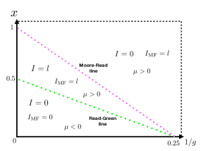
Figure 1: Mean-field phase diagram for $n=l$, as a function of $x$ and $g$. The topological invariant $I_{\mathrm{MF}}$, relative to a single Cooper pair, is reported, as well as the invariant $I$ from the exact wavefunction in Eq. (35). Notice the difference between MF and exact invariants in the phases above the Moore-Read line. The different length scale for the axes is chosen for sake of clarity of the picture. The Moore-Read line disappears in general out of integrability, if $n\neq l$.

The content in topology obtained using the MF wavefunctions can be probed also calculating the same quantity as in Eq. (32) in terms of the exact wavefunction $w_{\mathbf{k}}$ of a single Cooper pair, then considering again the limit $x=0$. We implicitly assume that fluctuations beyond MF do not change the MF phase diagram significantly; thus the solution of the Bethe-ansatz equations essentially leads to the same phase diagram. This hypothesis will not be contradicted in the following. The exact wavefunction, derived in Section II, reads, up to an unimportant multiplicative constant:

$$w_{{\bf k}}=\frac{(k_{x}-ik_{y})^{l}}{2\epsilon_{{\bf k}}-E}\,,$$ (35)

where $E$ is the pair energy (complex in general germanrev ), derived from the solution of the Richardson equations. The integral as in Eq. (32) can be recast as follows:

$$I=l^{2}\,\int_{0}^{\infty}\mathrm{d}u\,\frac{u^{(3l-1)}-E\bar{E}\,u^{(l-1)}}{(u^{l}+(u^{l}-E)(u^{l}-\bar{E}))^{2}}\,,$$ (36)

with $u=k^{2}$. The result of Eq. (36) is

$$\left\{\begin{array}[]{c}I=l\,\,\,\mathrm{if}\,\,\,E=0\\ {}\hfil\\ I=0\,\,\,\mathrm{if}\,\,\,E\neq 0\,.\end{array}\,\right.$$ (37)

An alternative derivation of the winding number $I$ is discussed in the Appendix B; this turns out to be useful also for the pure phase case in the Appendix C. Moreover, it would also be interesting to extend the calculation of $I$ to multi-pairs states, e. g., following the approaches in marquette2013 ; foster2013 .

Referring to the MF diagram in Fig. 1, the condition $E=0$ in (37) is fulfilled if $x=0$, at the intersection with the Moore-Read line, where $g=4$. This fact indicates that $I=l$ in the region between the Read-Green and the Moore-Read lines, while $I=0$ in the other phases. Therefore, $I$ matches the MF phase diagram, oppositely to $I_{\mathrm{MF}}$: indeed $I_{\mathrm{MF}}$ is nonvanishing also in the region to the right of the Moore-Read line, thus $I_{\mathrm{MF}}$ it does not detect this line. The described mismatch is indeed interesting, since it can indicate a general inability of the topological invariants from the MF wavefunctions to correctly detect some phases of (topological) insulators or superconductors. In our case, the mismatch occurs since the mass gap does not vanish on the MR line. It remains an open question whether the origin of the puzzle is due to integrability of the full model in Eq. (1). However, such interpretation is suggested by the fact that from the MF analysis the MR line seems generally absent for $n\neq l$, where integrability is broken (and no divergencies occur in the spectrum, a situation found instead in the presence of long-range Hamiltonian couplings, see lepori2016 and references therein lepori2017 ).

We note finally that in ortiz2010 it has been suggested, for the case $n=l=1$, that the Moore-Read line does not identify a genuine quantum phase transition, a possibility partly solving the mismatch mentioned above. However, the same result for $I$ (different from zero only at $E=0$) from the exact pair wavefunction, in sierralungo and in the present paper, seems to rule out this scenario.

V Discussion and conclusions

In this paper we have analyzed the physical features of a large set of superconductive models for which an exact solution is available, composed of two-dimensional systems with a factorized form for the momentum dependent interaction. Besides the known cases of the $s$-wave pairing, solved by Richardson Richardson63 , and $p$-wave pairing, discussed for the first time by Ibañez et al. in sierra09 , we have found that, in general, $l$-wave pairing is exactly solvable on a finite-size system, provided that the single particle dispersion is proportional to $k^{2n}$, with $n=l$.

Analyzing the integrable cases, we also found that the topological invariants calculated in the framework of the mean-field approach can not reproduce correctly the phase diagrams of the considered integrable models, in contrast to the corresponding invariants obtained from the exact (Bethe-ansatz) solutions. This discussion has shown the potential inadequacy of the mean-field topological invariants to predict the correct phase diagram of (topological) insulators and superconductors, at least in peculiar situations. In our case, the origin of this problem seems to be the (possible) presence of quantum phase transitions without vanishing of the mass gap, a feature possibly related to integrability. We notice that quite recently a change in topology without mass gap closing, in the presence of large interaction, was found numerically in capone2015 .

In the non-integrable cases $n\neq l$ (as well as for other perturbed models where interactions do not assume the special form of Eq. (1)), the exact wavefunctions analogous to Eq. (9) cannot be derived, because the Bethe-ansatz is not applicable, therefore only the the mean-field approach can be exploited. The reliability of this approach out of the integrable regime is suggested also by its prediction about the general absence of quantum phase transitions with nonvanishing mass gap.

Acknowledgements – The authors are pleased to thank Miguel Ibanez Berganza, Simone Paganelli, and German Sierra for useful discussions.

Appendix A Bethe-ansatz solution of equation (5)

The eigenvalue equation in (5) can be written as

$$\left(\left[H,\prod_{\nu=1}^{p}B_{J_{\nu}}^{\dagger}\right]-\mathcal{E}_{p}\prod_{\nu=1}^{p}B_{J_{\nu}}^{\dagger}\right)|0\rangle=0,$$ (38)

where the commutator on the left side expands as

$$\sum_{\nu=1}^{p}\left\{\left(\prod_{\eta=1}^{\nu-1}B_{J_{\eta}}^{\dagger}\right)\left[H,B_{J_{\nu}}^{\dagger}\right]\left(\prod_{\mu=\nu+1}^{p}B_{J_{\mu}}^{\dagger}\right)\right\}.$$ (39)

Using the relations

$$\left[b_{\mathbf{k}}^{\dagger}b_{\mathbf{k}},B_{J}^{\dagger}\right] =w_{\mathbf{k}}(J)b_{\mathbf{k}}^{\dagger},$$ (40)

$$\left[B_{0},B_{J}^{\dagger}\right] =\sum_{\mathbf{k}}z_{\mathbf{k}}^{*}w_{\mathbf{k}}(J)(1-2b_{\mathbf{k}}^{\dagger}b_{\mathbf{k}})$$

we find the expression for every single commutator appearing in Eq. (39):

$$\left[H,B_{J}^{\dagger}\right] = E_{J}B_{J}^{\dagger}+\sum_{\mathbf{k}}(2\epsilon_{\mathbf{k}}-E_{J})w_{\mathbf{k}}(J)b_{\mathbf{k}}^{\dagger}$$ (41)

$$-gB_{0}^{\dagger}\sum_{\mathbf{k}}z_{\mathbf{k}}^{*}w_{\mathbf{k}}(J)(1-2b_{\mathbf{k}}^{\dagger}b_{\mathbf{k}})\,.$$

Putting Eq. (41) in Eq. (39) and using the basic relation $H|0\rangle=0$, we find:

$$H|\Psi_{p}\rangle = \mathcal{E}_{p}|\Psi_{p}\rangle+\sum_{\nu=1}^{p}\left[\left(\sum_{\mathbf{k}}(2\epsilon_{\mathbf{k}}-E_{J_{\nu}})w_{\mathbf{k}}(J_{\nu})b_{\mathbf{k}}^{\dagger}-gB_{0}^{\dagger}\sum_{\mathbf{k}}z_{\mathbf{k}}^{*}w_{\mathbf{k}}(J_{\nu})\right)\left(\prod_{{\eta=1\atop\eta\neq\nu}}^{p}B_{J_{\eta}}^{\dagger}\right)\right]|0\rangle$$ (42)

$$+\sum_{\nu=1}^{p}\left\{\left(\prod_{\eta=1}^{\nu-1}B_{J_{\eta}}^{\dagger}\right)2gB_{0}^{\dagger}\left(\sum_{\mathbf{k}}z_{\mathbf{k}}^{*}w_{\mathbf{k}}(J_{\nu})b_{\mathbf{k}}^{\dagger}b_{\mathbf{k}}\right)\left(\prod_{\mu=\nu+1}^{p}B_{J_{\mu}}^{\dagger}\right)\right\}|0\rangle\,.$$

In the last term of Eq. (42), we want to commute the operator $b_{\mathbf{k}}^{\dagger}b_{\mathbf{k}}$ to the extreme right, where it annihilates the vacuum $|0\rangle$. To this aim, we write this term as

$$\sum_{\nu=1}^{p}\left\{2gB_{0}^{\dagger}\left(\prod_{\eta=1}^{\nu-1}B_{J_{\eta}}^{\dagger}\right)\sum_{\mu=\nu+1}^{p}\left\{\left(\prod_{\eta^{\prime}=\nu+1}^{\mu-1}B_{J_{\eta^{\prime}}}^{\dagger}\right)\left[\sum_{\mathbf{k}}z_{\mathbf{k}}^{*}w_{\mathbf{k}}(J_{\nu})b_{\mathbf{k}}^{\dagger}b_{\mathbf{k}},B_{J_{\mu}}^{\dagger}\right]\left(\prod_{\mu^{\prime}=\mu+1}^{p}B_{J_{\mu^{\prime}}}^{\dagger}\right)\right\}\right\}|0\rangle.$$ (43)

At this point, it is crucial to use the following manageable form for the commutator in Eq. (43):

$$\left[\sum_{\mathbf{k}}z_{\mathbf{k}}^{*}\,w_{\mathbf{k}}(J_{\nu})\,b_{\mathbf{k}}^{\dagger}b_{\mathbf{k}},B_{J_{\mu}}^{\dagger}\right]=\sum_{\mathbf{k}}z_{\mathbf{k}}^{*}\,w_{\mathbf{k}}(J_{\nu})w_{\mathbf{k}}(J_{\mu})\,b_{\mathbf{k}}^{\dagger}\,.$$ (44)

In general, for every $\mu$ and $\nu$, we want to express Eq. (44) in the form $C_{\mu,\nu}B_{J_{\nu}}^{\dagger}+D_{\mu,\nu}B_{J_{\mu}}^{\dagger}$, where $C_{\mu,\nu}$ and $D_{\mu,\nu}$ are some coefficients. For this reason, we impose the condition

$$\sum_{\mathbf{k}}z_{\mathbf{k}}^{*}w_{\mathbf{k}}(J_{\nu})w_{\mathbf{k}}(J_{\mu})b_{\mathbf{k}}^{\dagger}=C_{\mu,\nu}B_{J_{\nu}}^{\dagger}+C_{\nu,\mu}B_{J_{\mu}}^{\dagger}\,,$$ (45)

where we have used the symmetry under the exchange $\nu\leftrightarrow\mu$. Assuming that Eq. (45) is correct, then we find that the eigenvalue equation (42) holds, provided that

$$1-g\sum_{\mathbf{k}}\frac{|z_{\mathbf{k}}|^{2}}{2\epsilon_{\mathbf{k}}-E_{J_{\nu}}}+2g\sum_{\mu=1(\neq\nu)}^{p}C_{\nu,\mu}=0\,,$$ (46)

where we have used the expression for the wave function $w_{\mathbf{k}}(J)=\frac{z_{\mathbf{k}}}{2\epsilon_{\mathbf{k}}-E_{J}}$. Equation (45) gives

$$(2\epsilon_{\mathbf{k}}-E_{J_{\mu}})C_{\mu,\nu}+(2\epsilon_{\mathbf{k}}-E_{J_{\nu}})C_{\nu,\mu}=|z_{\mathbf{k}}|^{2}$$

with two different kind of solutions:

1. s-wave. In this case $|z_{\mathbf{k}}|^{2}=1$ and $C_{\mu,\nu}=-C_{\nu,\mu}=(E_{J_{\nu}}-E_{J_{\mu}})^{-1}$. Thus, from (46) we get the well-known Richardson equation Eq. (11), with no restrictions on $\epsilon_{\mathbf{k}}$. Notice that the condition $|z_{\mathbf{k}}|^{2}=1$ is more general than the $s$-wave case $z_{\mathbf{k}}=1$.

2. l-wave. In this case, $z_{\mathbf{k}}=(k_{x}-ik_{y})^{l}$ depends on $\mathbf{k}$ (for $l\neq 0$) and the coefficients are given by

   $$C_{\mu,\nu}=\frac{|z_{\mathbf{k}}|^{2}}{2\epsilon_{\mathbf{k}}}\frac{E_{J_{\nu}}}{E_{J_{\nu}}-E_{J_{\mu}}}\,,$$ (47)

   but we must have $|z_{\mathbf{k}}|^{2}\propto\epsilon_{\mathbf{k}}$ to have an $C_{\mu,\nu}$ independent of $\mathbf{k}$. As a consequence, after the substitution $|z_{\mathbf{k}}|^{2}=\alpha\,\epsilon_{\mathbf{k}}$, Eq.(46) becomes Eq. (12).

Appendix B Alternative calculation of $I$

In this appendix we discus an alternative derivation of the winding number $I$, which is also useful for the pure phase case in the Appendix C, that can be performed by analyzing directly the map $\omega_{\mathbf{k}}$ in the case of real $E$. In order to do that, we first separate Eq. (35) as

$$\omega_{\mathbf{k}}=\big{(}f_{-}(k)+f_{+}(k)\big{)}\,e^{i\phi_{k}l}$$ (48)

with $f_{-}(k)=\frac{k^{l}}{k^{2l}-E}$, $k<E^{1/2l}$, and $f_{+}(k)=\frac{k^{l}}{k^{2l}-E}$, $k>E^{1/2l}$.
The part $f_{+}(k)\,e^{i\phi_{k}l}$ gives a contribution $I_{+}=l$ to $I$, since $f_{+}(k)$ is monotonic in $k$ and assumes values $[0,\infty)$, so that $f_{+}(k)\,e^{i\phi_{k}l}$ covers $l$ times (because of the phase $l\,\phi_{k}$) the entire plane $R^{2}\sim S^{2}$ (the identification relying again on the stereographic projection).
Assuming now that $E\neq 0$, we put $k=1/p$ in $f_{-}(k)$ , obtaining $f_{-}(p)=-\frac{1}{E}\,\frac{p^{l}}{p^{2l}-E}=-f_{+}(p)$, with $p>E^{1/2l}$. Apart from the unimportant multiplicative factor $E^{-1}$, we can write (renaming $p\equiv k$)

$$\omega_{\mathbf{k}}=\big{(}f_{-}(k)-f_{-}(k)\big{)}\,e^{i\phi_{k}l}\,=0\,$$ (49)

showing that $I=0$ if $E\neq 0$. The minus sign in $f_{-}(p)$, responsible for the vanishing result for $I$, is related to the fact that, for $k$ varying, $f_{+}(k)$ and $f_{-}(k)$ span the space $R^{2}\sim S^{2}$ in the opposite sense.
The situation is different if $E=0$: in this case we get only

$$\omega_{\mathbf{k}}=f_{+}(k)\,e^{i\phi_{k}l}$$ (50)

and $I=I_{+}=l$.

Appendix C Pure phase gap

We can also calculate the topological index $I$ in the case when $\Delta(k)=e^{i\phi_{\hat{k}}l}$. In this case, we have shown in Sec. II that we have integrability, no matter what the particular single particle dispersion $\epsilon_{\mathbf{k}}$ is; therefore, we assume again $\xi_{(l)}(k)=k^{2l}$. The exact wave function reads, in momentum space and up to an unimportant multiplicative constant,

$$\omega_{\mathbf{k}}=\frac{(k_{x}-ik_{y})^{l}}{k^{l}\,\big{(}2\epsilon_{\mathbf{k}}-E\big{)}}\,,$$ (51)

In this case, we obtain:

$$I=2l^{2}\,\int_{0}^{\infty}\mathrm{d}k\,\frac{k^{(2l-1)}\Big{[}2k^{2l}-(E+\bar{E})\Big{]}}{(1+(k^{2l}-E)(k^{2l}-\bar{E}))^{2}}\,.$$ (52)

This integral yields $I=\frac{l}{|E|^{2}+1}$, a pretty unexpected result, since in general a integer winding number should be expected. However this result can be explained quite naturally by analyzing the map (51) directly. This map can be expressed as:

$$\omega_{\mathbf{k}}=\frac{1}{k^{2l}-E}\,e^{i\phi_{k}l}\,.$$ (53)

As for (35), we can write again:

$$\omega_{\mathbf{k}}=\big{(}f_{-}(k)+f_{+}(k)\big{)}\,e^{i\phi_{k}l}\,$$ (54)

with $f_{-}(k)=\frac{1}{k^{2l}-E}$, $k<E^{1/2l}$, and $f_{+}(k)=\frac{1}{k^{2l}-E}$, $k>E^{1/2l}$. We notice that $f_{-}(k)\,e^{i\phi_{k}l}$ is homotopic to a constant map $\tilde{f}_{-}(k)=c$, since $f_{-}(k)=(-\infty,-\frac{1}{E}]$ (the minus sign is re-absorbable in the phase $\phi_{k}$ ) and not every point of the target stereographic plane $R^{2}$ is covered by $f_{-}(k)\,e^{i\phi_{k}l}$. Then we can write

$$\omega_{\mathbf{k}}=\big{(}f_{-}(k)+f_{+}(k)\big{)}\,e^{i\phi_{k}l}\sim f_{-}(k)\,e^{i\phi_{k}l}$$ (55)

(here the symbol $\sim$ means "continuously deformable to"). Since again $f_{+}(k)=[0,\infty)$ and is monotonic, it yields a contribution $I_{+}=l$ to $I$ for every value of $E$. However $f_{-}(k)$ gives a non vanishing contribution to $I$, covering a part of the sphere with area

$$I_{-}=-\frac{1}{\pi}\,\int_{0}^{\frac{1}{E}}\mathrm{d}k\,\frac{2\pi\,k}{(1+k^{2})^{2}}=-\frac{E^{2}}{E^{2}+1}\,,$$ (56)

where the minus sign appears since $|f_{-}(k\to\infty)|\to\infty$. This contribution sums up to $I_{+}$, giving the result (52):

$$I=I_{+}+I_{-}=l-l\,\frac{E^{2}}{E^{2}+1}=l\,\frac{E^{2}}{E^{2}+1}\,.$$ (57)

In spite of the value of $I$, the real winding number related to (51) is $\tilde{I}=I_{+}=l$, since we know that $f_{-}(k)$ is homotopic to a constant map, a fact also resulting in a value of $|I_{-}|$ smaller than 1.
This result matches the fact that the BCS case and the (53) case are linked by the transformation in the gap $\Delta\to\Delta(k)=\Delta\,e^{i\phi_{k}l}$. However, this map is continuous but not invertible, wrapping $l$ times: this is the reason of $\tilde{I}=l$.

In conclusion, the case (53) describes a phase with winding number $I=l\frac{N}{2}$ (with $\frac{N}{2}$ being the number of Cooper pairs in the ground-state). However, the energy of Bogoliubov quasiparticles is the same as in the BCS case, and always gapped; thus no phase transitions arise and the system is always in a phase with nontrivial topology.

References

- (1) M. Alford, A. Schmitt, K. Rajagopal, and T. Schäfer, Rev. Mod. Phys. 80, 1455 (2008).
- (2) R. Anglani, R. Casalbuoni, M. Ciminale, N. Ippolito, R. Gatto, M. Mannarelli, and M. Ruggieri, Rev. Mod. Phys. 86, 509 (2014).
- (3) J. Bardeen, L. N. Cooper, and J. R. Schrieffer, Phys. Rev. 108, 1175 (1957).
- (4) R. W. Richardson, Phys. Lett. 3, 277 (1963); ibid. 5, 82 (1963).
- (5) H.-Q. Zhou, J. Links, R. H. McKenzie, and M. D. Gould, Phys. Rev. B 65, 060502(R) (2002).
- (6) J. von Delft and R. Poghossian, Phys. Rev. B 66, 134502 (2002).
- (7) J. Dukelsky, S. Pittel, and G. Sierra, Rev. Mod. Phys. 76, 643 (2004).
- (8) C. Dunning, M. Ibanez, J. Links, G. Sierra, and S. Y. Zhao, J. Stat. Mech. P08025 (2010).
- (9) G. Ortiz, J. Dukelsky, E. Cobanera, C. Esebbag, and C. Beenakker, Phys. Rev. Lett. 113, 267002 (2014).
- (10) J. Dukelsky, C. Esebbag, and S. Pittel, Phys. Rev. Lett. 88, 062501 (2002).
- (11) M. Ibañez, J. Links, G. Sierra, and S. Y. Zhao, Phys. Rev. B 79, 180501(R) (2009).
- (12) M. Van Raemdonck, S. De Baerdemacker, and D. Van Neck, Phys. Rev. B 89, 155136 (2014).
- (13) G. Ortiz, R. Somma, J. Dukelsky, and S. M. A. Rombouts, Nucl. Phys. B 707, 421 (2005).
- (14) S. M. A. Rombouts, J. Dukelsky, and G. Ortiz, Phys. Rev. B 82, 224510 (2010).
- (15) J. Dukelsky, S. Lerma H., L. M. Robledo, R. Rodriguez-Guzman, and S. M. A. Rombouts, Phys. Rev. C 84, 061301 (2011).
- (16) F. Pan, J. P. Draayer, and W. E. Ormand, Phys. Lett. B 422 1, (1998).
- (17) L. Fidkowski, J. Alicea, N. Lindner, R. M. Lutchyn, and M. P. A. Fisher, Phys. Rev. B 85, 245121 (2012).
- (18) I. Affleck, and D. Giuliano, J. Stat. Mech. P06011 (2013).
- (19) I. Affleck, and D. Giuliano, J. Stat. Phys. 157 4 (2014).
- (20) J. N. Fuchs, A. Recati, and W. Zwerger, Phys. Rev. Lett. 93, 090408 (2004).
- (21) P. A. Lee, N. Nagaosa, and X.-G. Wen, Rev. Mod. Phys. 78, 17 (2006).
- (22) Y. Cao, V. Fatemi, S. Fang, K. Watanabe, T. Taniguchi, E. Kaxiras, and P. Jarillo-Herrero, Nature 556, 80 (2018).
- (23) G. E. Volovik, in Quantum Analogues: From Phase Transitions to Black Holes and Cosmology Lect. Notes Phys. 718, 31 (2007); ibid., The Universe in a Helium Droplet, second edition, Oxford University Press (2009).
- (24) A. P. Mackenzie and Y. Maeno, Rev. Mod. Phys. 75, 657 (2003).
- (25) Y. Maeno, S. Kittaka, T. Nomura, S. Yonezawa, and K. Ishida, J. Phys. Soc. Jpn. 81, 011009 (2012).
- (26) U. E. Israelsson, B. C. Crooker, H. M. Bozler, and C. M. Gould, Phys. Rev. Lett. 56, 2383 (1986).
- (27) J. P. Davis, H. Choi, J. Pollanen, and W. P. Halperin, Phys. Rev. Lett. 97, 115301 (2006).
- (28) M. Lewenstein, A. Sanpera, and V. Ahufinger, Ultracold atoms in optical lattices: simulating quantum many-body systems, Oxford University Press (2012).
- (29) L. Mathey, S.-W. Tsai, and A. H. Castro Neto, Phys. Rev. B 75, 174516 (2007).
- (30) O. Dutta and M. Lewenstein, Phys. Rev. A 81, 063608 (2010).
- (31) W.-C. Lee,1, C. Wu,, and S. Das Sarma, Phys. Rev. A 82, 053611 (2010).
- (32) L. Mao, J. Shi, Q. Niu, and C. Zhang, Phys. Rev. Lett. 106, 157003 (2011).
- (33) N. Hao, G. Liu, N. Wu, J. Hu, and Y. Wang, Phys. Rev. A 87, 053609 (2013).
- (34) H.-H. Hung, W.-C. Lee, and C. Wu, Phys. Rev. B 83, 144506 (2011).
- (35) A. Boudjemaa, J. Low Temp. Phys. 189, 76 (2017).
- (36) M. R. Zirnbauer, J. Math. Phys. 37, 4986 (1996).
- (37) A. Altland and M. R. Zirnbauer, Phys. Rev. B 55, 1142 (1997).
-
(38)
A. P. Schnyder, S. Ryu, A. Furusaki, A. W. W. Ludwig,
AIP Conf. Proc. 1134, 10 (2009),
arXiv:0905.2029. - (39) S. Ryu, A. P. Schnyder, A. Furusaki, A. W. W. Ludwig, New Journ. Phys. 12, 065010 (2010).
- (40) J. von Delft and F. Braun, cond-mat/9911058. Proceedings of the NATO ASI Quantum Mesoscopic Phenomena and Mesoscopic Devices in Microelectronics, Ankara/Antalya, Turkey, June 1999, Eds. I.O. Kulik and R. Ellialtioglu, Kluwer Ac. Publishers, Dordrecht, 2000, p. 361.
- (41) G. Grosso and G. Pastori Parravicini, Solid State Physics, Elsevier Ltd, Oxford (2014).
- (42) J. F. Annett, Superconductivity, Superfluids, and Condensates, Oxford University Press (2004).
- (43) A. Birrell, P. S. Isaac, J. Links, Inverse Problems 28 035008 (2012); arXiv:1112.1740.
- (44) I. Marquette and J. Links, Nucl. Phys. B 866, 3 378 (2013).
- (45) L. Campos Venuti and M. Roncaglia Phys. Rev. A 81, 060101(R) (2010).
- (46) N. Read and D. Green, Phys. Rev. B 61, 10267 (2000).
- (47) J. Links, I. Marquette, and A. Moghaddam, J. Phys. A: Math. Theor. 48, 374001 (2015).
- (48) This is also suggested by the fact that only if (see Eq. (25)).
- (49) B. A. Bernevig with T. L. Hughes, Topological Insulators and Topological Superconductors, Princeton University Press (2013).
- (50) If a lattice realization for Eq. (1) is considered, the same integral must be performed on the corresponding Brillouin zone.
- (51) P. W. Anderson, Phys. Rev. 110, 827 (1958); ibid. 112, 1900 (1958).
- (52) M. S. Foster, M. Dzero, V. Gurarie, and E. A. Yuzbashyan, Phys. Rev. B 88, 104511 (2013).
- (53) L. Lepori and L. Dell’Anna, New J. Phys. 19, 103030 (2017).
- (54) L. Lepori, D. Giuliano, and S. Paganelli, Phys. Rev. B 97, 041109(R) (2018).
- (55) A. Amaricci, J. C. Budich, M. Capone, B. Trauzettel, and G. Sangiovanni, Phys. Rev. Lett. 114, 185701 (2015).