Probing finite coarse-grained virtual Feynman histories with sequential weak values
Abstract
Feynman’s sum-over-histories formulation of quantum mechanics has been considered a useful calculational tool in which virtual Feynman histories entering into a coherent quantum superposition cannot be individually measured. Here we show that sequential weak values, inferred by consecutive weak measurements of projectors, allow direct experimental probing of individual virtual Feynman histories thereby revealing the exact nature of quantum interference of coherently superposed histories. Because the total sum of sequential weak values of multi-time projection operators for a complete set of orthogonal quantum histories is unity, complete sets of weak values could be interpreted in agreement with the standard quantum mechanical picture. We also elucidate the relationship between sequential weak values of quantum histories with different coarse-graining in time and establish the incompatibility of weak values for non-orthogonal quantum histories in history Hilbert space. Bridging theory and experiment, the presented results may enhance our understanding of both weak values and quantum histories.
pacs:
03.65.Ta, 03.65.Ca, 03.65.UdIn this work, we revisit the important yet controversial concept of quantum weak values and elucidate the relationship between Aharonov’s two-state vector formalism and Feynman’s sum-over-histories. This interesting relationship resonates with past works which studied non-demolition and continuous quantum measurements Braginsky and Khalili (1992, 1996); Mensky (1993, 2000), while connecting them with path integration Mensky (1979). Recently, the above relationship was further analyzed and strengthened by different researchers Duprey and Matzkin (2017); Matzkin (2012, 2015); Sokolovski (2016a, b, 2017), but here we focus on the notion of sequential weak values as a pivotal issue, which has not been mentioned before in the above literature. In particular, we show that sequential weak values are able to probe directly the quantum probability amplitudes along individual virtual Feynman histories thereby possibly supporting their physical meaningfulness. Conversely, we utilize the mathematical constraints behind Feynman summation in order to provide rules for consistent interpretation of experimentally measured weak values.
I Preliminaries
To begin with, we succinctly describe a finite coarse-grained Feynman’s sum-over-histories procedure applicable to any experiment performed with a finite precision.
Definition 1.
(Quantum history) Quantum histories from an initial time to a final time are constructed at different times with the use of complete sets of projection operators , , , , , which at each single time span the -dimensional Hilbert space of the system , , , , , . Using the symbol for tensor products at different times, we can write each quantum history as a projection operator in history Hilbert space , where is a copy of the standard Hilbert space of the physical system at time Gell-Mann and Hartle (1990, 1993); Griffiths (1984, 1993, 2003); Halliwell (1995); Hartle (1993). By construction there are orthogonal quantum histories ( for ) that span the history Hilbert space .
Definition 2.
(Chain operator) To each quantum history in history Hilbert space , there is a corresponding chain operator in standard Hilbert space , where is the time evolution operator from to .
Definition 3.
(History probability amplitude) The quantum probability amplitude propagating along a quantum history from an initial quantum state at to a final quantum state at is given by . Expanding the projectors using their corresponding unit eigenvectors as , allows us to rewrite the chain operator as . Introducing the Feynman propagators from to as , further gives . The quantum probability amplitude for the history is then a product of Feynman propagators (each of which is a complex-valued function) .
Definition 4.
(Feynman’s sum-over-histories) The quantum probability amplitude for a quantum transition from an initial quantum state at to a final quantum state at is given by the sum over a complete set of orthogonal quantum histories , , which span the history Hilbert space of the system . Inclusion of among the projectors of the complete set at and among the projectors of the complete set at eliminates a large number of quantum histories that start or end with projection operators respectively orthogonal to or , and consequently have zero contribution, , to the Feynman sum. Thus, Feynman summation will produce identical result if it is performed over all orthogonal quantum histories of the type , which form a complete set for the intermediate times . The usage of the Feynman sum , reduces the complete history Hilbert space for Feynman summation to -dimensional due to consideration of only the copies of the -dimensional Hilbert space at intermediate times .
Theorem 5.
Discontinuous Feynman histories have zero contribution to the total Feynman sum . Feynman summation over a complete set of continuous quantum histories generates the same result as the total Feynman sum over all histories.
Proof.
The quantum probability amplitude propagating along an arbitrary quantum history , is calculated from the inner product of the corresponding chain operator . The quantum time evolution operators are continuous in space and have non-zero product only between spatially connected projectors and . The presence of two consecutive disconnected projectors and anywhere in the quantum history effectively zeroes it through the presence of .∎
Next, let us briefly review the concept of weak values in Aharonov’s two-state vector formalism. Experimental measurement of weak values requires a weak coupling between the measured system and the measuring pointer, multiple experimental runs, post-selection and calculation of averages Aharonov et al. (1988); Jozsa (2007); Aharonov et al. (2014); Dressel et al. (2014). Because unknown quantum states cannot be cloned Wootters and Zurek (1982), weak values are meaningful only if one is given an ensemble of quantum systems that are all prepared in the same initial quantum state upon which measurements are made and only those results are analyzed that end up with a certain post-selected final state .
Definition 6.
(Weak value) The weak value of an operator at any moment of time during the evolution from initial state at an initial time to a final state at a final time is
| (1) |
where and . In Aharonov’s two-state vector formalism the pre-selected state evolves forward in time with the time evolution operator and the post-selected state evolves backward in time with the time evolution operator , namely , so that one employs both a bra and a ket at the same time at which is measured Aharonov et al. (2017a).
Definition 7.
Weak values are complex-valued, however, both the real and the imaginary parts of the weak values defined by Eqs. 1 and 2 can be experimentally measured with the use of weak measurements (cf. Aharonov and Vaidman (1990); Jozsa (2007); Mitchison et al. (2007); Svensson (2013); Piacentini et al. (2016)).
The mathematical expressions (1) and (2) of weak values arise in the approximate calculation of the pointer shifts when multiplying truncated power series expansions of the exponentiated interaction Hamiltonians between the measured system and the measuring pointers at -times (see Appendix).
Before we present the main results of this work, we wish to address two technical points. First, we note that all the above was defined for arbitrary operators, but in the next section we shall focus on (not necessarily commuting) projection operators as commonly done when discussing sum over histories. Second, for making the notion of weak measurement feasible, the physical systems in question are assumed to exist in a fine-grained Hilbert space, which can be taken to be either finite dimensional and consisting of Planck scale units, or infinitely dimensional (so that standard differential and integral calculus applies) but effectively described by a finite, coarse-grained Hilbert space. We shall henceforth assume an -dimensional Hilbert space, applicable to the two cases above.
II Main results
Now we are ready to demonstrate the tight relationship between Aharonov’s two-state vector formalism and Feynman’s sum-over-histories. We will also elucidate the meaning and properties of sequential weak values of multi-time projection operators.
Theorem 8.
The sequential weak value of multi-time projection operators at times is equal to the quantum probability amplitude propagating along the individual Feynman history , divided by the total quantum probability amplitude of the Feynman sum , over a complete set of quantum histories from to .
Proof.
The quantum probability amplitude for the individual Feynman history is given by the corresponding chain operator
| (3) | |||||
which is exactly the numerator in Eq. 2. Thus, two-state vectors of multi-time projection operators in Aharonov’s two-state vector formalism are equivalent to quantum probability amplitudes propagating along a Feynman history. Similarly, the total quantum probability amplitude for the Feynman sum over all quantum histories is given by the sum of all chain operators
| (4) | |||||
which is exactly the denominator in Eq. 2. Eq. 4 also shows that the denominator of weak values in Aharonov’s two-vector state formalism is a disguised two-state vector of multi-time identity operator. Dividing Eq. 3 by 4 gives
| (5) |
Because the ordinary weak values (Eq. 1) serve as a special single-time case of sequential weak values (Eq. 2), Eq. 5 holds true for Feynman histories with a single intermediate time as well. Interestingly, Eq. 5 even makes sense for the trivial case with no intermediate time points in the quantum history where it returns the weak value of the identity operator . ∎
Equation 5 provides a direct link between the theory of weak values in weak measurements, which require a small, but strictly non-zero perturbation, i.e. , and Feynman sum-over-histories, which exactly quantifies quantum interference of virtual quantum histories without any external coupling, i.e. . Thus, we demonstrate unambiguously that weak values are not an artifact arising from the small perturbation parameter , but are rather descriptive properties of quantum systems that are exactly defined at . For example, in experimental measurement of a single-time weak value, the pointer shift is or plus a higher order correction term (see Appendix), hence due to the pointer shift dependence on , the weak value can be measured with arbitrarily small, but non-zero error . By considering the theory of weak measurement alone, where weak values correspond to, and are interpreted as, average pointer shifts Wu (2013); Shomroni et al. (2013), one may be misled into thinking that the weak value is only defined as a limit at , while at due to the zero pointer shift there is no weak value to be extracted. The mathematical technique for Feynman summation, may however provide a proper context for better understanding the meaning of weak values as relative quantum probability amplitudes at zero disturbance. To measure such amplitudes, which by definition are at zero disturbance (), Aharonov et al. Aharonov et al. (1988) developed the weak measurement scheme that allows for controlling the error in the measurement of the weak values, making the error arbitrarily small for sufficiently small .
From the measurability of weak values, we can prove that quantum probability amplitudes along individual virtual Feynman histories entering into a quantum superposed Feynman sum are also measurable given an ensemble of quantum systems that are all prepared in the same initial state .
Theorem 9.
Measured sequential weak value of multi-time projection operators could be converted (up to a pure phase factor ) into quantum amplitude for the individual quantum history entering into a quantum superposed Feynman sum via multiplication of the weak value by the positive square root of the experimentally measured quantum probability for an initial pre-selected state to end at the final post-selected state .
Proof.
From Eqs. 2 and 3 we can express through the weak value as
| (6) |
Since is a complex number it can be expressed as a product of its real-valued modulus times a pure phase . Thus, for the quantum probability amplitude, we have
| (7) |
In the weak value formula (Eq. 5), the pure phase is canceled down from the numerator and denominator. Because removing the pure phase from each of the superposed quantum histories entering into the Feynman sum
| (8) |
does not affect the quantum interference effects, the weak values can be used to directly probe Feynman’s sum-over-histories formulation of quantum mechanics. ∎
Sequential weak values are defined with the use of quantum observables , , , at times (Definition 7). Therefore, in general, sequential weak values are not the normalized quantum probability amplitudes propagating along quantum histories. The spectral decompositions of observables in Eq. 2 are given by , , , , where , , , are indices that may vary independently, , , , are sets of eigenvalues and , , , are sets of corresponding projection operators for the eigenvectors of , , . Consequently, a general sequential weak value will be a weighted sum of quantum probability amplitudes for Feynman histories, each of which is multiplied by a non-normalized weight given by a product of eigenvalues . To illustrate the point, let us set to suppress all time evolution operators i.e. , thereby obtaining for the sequential weak value:
Such a general sequential weak value is not subject to the Born rule and does not generate a probability for observing the corresponding quantum (Feynman) history (defined with the projectors only). Our main point is that by restricting the general observables down to projection operators in sequential weak values, one can connect Feynman sum-over-histories approach with the fruitful area of weak measurements and weak values. Note that for each sequential weak value of multi-time projection operators, there is a corresponding Feynman history and the probability for measuring that history through a series of strong measurements at times is given by the Born rule, i.e. .
Sequential weak values of multi-time projection operators are able to directly probe the quantum probability amplitudes along individual virtual Feynman histories that enter into a quantum superposed Feynman sum . Because Feynman’s sum-over-histories approach to quantum mechanics works for a complete set of orthogonal quantum histories in the history Hilbert space, we can derive an exact value for the sum of the corresponding sequential weak values:
Theorem 10.
For a complete set of orthogonal quantum histories that span the history Hilbert space of a quantum transition with non-zero probability, the complex sequential weak values sum up to unity .
Proof.
Quantum transition with non-zero probability ensures that all weak values are finite due to non-zero denominator, . Taking the sum over all histories on both sides of Eq. 5 gives
| (10) | |||||
∎
The converse of Theorem 10 is not true, namely, the fact that the weak values for a set of quantum histories sum to unity does not imply that the set of quantum histories is complete.
Corollary 11.
Sequential weak values of multi-time projection operators are not conditional probabilities, but relative probability amplitudes . Weak values are measured by the mean value of the pointer shift of the measuring device, which makes quantum probability amplitudes measurable provided that one is given an ensemble of quantum systems that are all prepared in the same initial state .
Theorem 12.
Analysis of quantum interference effects within a complete set of mutually orthogonal quantum histories from to is consistent with the standard quantum mechanical picture.
Proof.
By the completeness of the set of quantum histories entering into the Feynman sum, we are guaranteed to obtain identity operators for all intermediate times . Therefore, the corresponding sum of chain operators is
| (11) | |||||
Expressing in terms of the Hamiltonian shows that the total Feynman sum is just the standard quantum probability amplitude that one would obtain from unitary evolution according to the Schrödinger equation
| (12) |
Noteworthy, orthogonality of the corresponding chain operators was not assumed, which shows that Feynman summation is not equivalent to the decoherent (consistent) histories approach that requires for Gell-Mann and Hartle (1990, 1993); Griffiths (1984, 1993, 2003); Hartle (1993); Halliwell (1995). ∎
Analysis of weak values corresponding to a complete set of mutually orthogonal quantum histories that span the history Hilbert space avoids paradoxes because the orthogonality ensures that one weak value cannot be used to infer claims for more than one history, and the completeness of the set of histories implies consistency with the Schrödinger equation (Theorem 12). Due to the linearity of sums in quantum mechanical inner products , Feynman’s approach provides a natural language for discussion of quantum interference effects between individual quantum histories Cotler and Wilczek (2015, 2016, 2017); Nowakowski (2017). Running the proof of Theorem 12 backwards also shows that starting from the Schrödinger equation (Eq. 12), one could obtain correct quantum probability amplitudes by inserting identity operators at intermediate time points and then summing over all quantum histories spanning the history Hilbert space (Eq. 11).
Theorem 13.
Sequential weak values evaluated at different number of intermediate times correspond to different coarse-grainings of the history Hilbert space. Consequently, -time sequential weak values are quantum superpositions of -time sequential weak values.
Proof.
The sequential weak value corresponds to a -time coarse-grained Feynman history The time tensor between projectors at and contains a hidden identity operator at time , which when resolved as a sum of orthogonal projectors gives a quantum superposition of -time fine-grained Feynman histories . Calculating the quantum probability amplitudes from the corresponding chain operators and applying the weak value formula (Eq. 5) gives
| (13) | |||||
∎
Definition 14.
Incompatible weak values are (sequential) weak values whose corresponding quantum histories are not orthogonal in history Hilbert space.
The main goal of Feynman sum-over-histories is to predict probabilities for quantum events to occur. To obtain valid quantum probabilities, however, the Feynman summation should not be performed over all quantum histories in the history Hilbert space , but only over a complete set of orthogonal histories that span . The non-orthogonal quantum histories of incompatible weak values cannot interfere with each other because this would overcount certain histories in the Feynman sum more than once, rendering incorrect quantum probability for the transition from to for almost all physically valid Hamiltonians. Indeed, consider a complete set of quantum histories to which is added an extra non-orthogonal history . In the general case with , for coherent superposition, we will have
| (14) |
and for incoherent superposition
| (15) |
Conservation of quantum probability will not be violated only in the special case where . Thus, one may be tempted to give a special status to non-orthogonal quantum histories with zero weak values and interpret them unconditionally. This, however, would contradict the mathematical principles that ensure the status of Feynman sum-over-histories as one of several equivalent formulations of quantum mechanics. In particular, notice that the orthogonality of quantum histories is independent of the Hamiltonian and the correctly constructed Feynman sum will always return the correct transition amplitude for any . On the other hand, having a zero quantum probability amplitude, , is a Hamiltonian-dependent condition, which means that summation over non-orthogonal histories cannot return the correct transition amplitudes for all physically valid Hamiltonians, hence it cannot be a fundamental principle upon which to build quantum mechanics.
III Application
We illustrate the power of the presented theorems with the analysis of a concrete interferometric setup shown in Fig. 1. The transition probability amplitude from the source to the detector can be easily calculated with the use of actual Feynman summation and various weak values can be determined with the use of Theorem 8. Among the three alternative ways to calculate the Feynman sum, namely with the use of matrix exponential of the Hamiltonian , time development operators or Feynman propagators , the latter one is computationally most effective. Utilizing Theorem 5, there are only nine coarse-grained continuous quantum histories from to that need to be summed over with their corresponding quantum probability amplitudes :
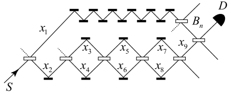
For , the single-time weak value is able to extract the quantum probability amplitude along history , however, for histories – one needs to use sequential weak values of multi-time projection operators that uniquely identify each history inside the three inner interferometers: , , , , , , , .
From Eq. 5 it can be seen that once the fine-grained quantum histories are resolved, adding projectors at extra times does not change the weak values, e.g. . On the other hand, reducing the number of projectors selects quantum superpositions of Feynman histories, e.g.:
Thus, weak values are descriptive properties of the measured quantum system that depend on the quantum history of interest (Theorem 8). Feynman’s sum-over-histories emphasizes the natural occurrence of pre- and post-selection in quantum mechanics. Moreover, it also reveals that in some sense sequential weak values are primitive and more fundamental than single-time weak values, which are in fact superposed sums of sequential weak values, e.g.: . This was similarly shown for multipartite weak values Aharonov et al. (2017b).
Weak values measure different Feynman histories from the source to the detector , but only sets of weak values that complete the history Hilbert space can be consistently interpreted together. For example, taken together and state that the quantum has reached the detector through but not through , and this is consistent because all fine-grained histories – are accounted for. In contrast, when taken together , , , , , , , and state that the quantum has not passed through and , yet it has been at , , and ; the apparent discontinuity arises from overcounting five times each of –. Thus, Theorem 13 explicitly addresses the controversy between Svensson and Vaidman Svensson (2015); Ben-Israel and Vaidman (2017); Svensson (2017) utilizing the general applicability of weak values for determining the history of a quantum system.
While weak values substantiate the physical nature of virtual Feynman histories through measurable pointer shifts, the mathematical constraints for correct Feynman summation elucidate the meaning and properties of weak values. Sequential weak values reflect the unique character of temporal correlations, as was also shown by Avella et al. Avella et al. (2017). Consider as another example, an experimenter changing the number of beam splitters from to on the history through , while measuring devices record the weak values at or . The presence of extra beamsplitters on arm is felt by the weak measuring devices at arm or as they measure the very large weak values and . In other words, the weak measurement devices at arms or somehow feel the photon exploration of alternative quantum histories Danan et al. (2013). Thus, the weak value measured through some weak coupling to a measuring pointer at one location integrates information about the presence of other devices at different locations in the interferometer through the change of the total Feynman sum . Of course, weak values cannot be used for superluminal communication since to extract the weak values from the recorded data, experimenters located at or need to know which photons were detected by .
IV Concluding remarks
Our results are consistent with a recent work by Sokolovski Sokolovski (2016b), but we have extended it in scope and generality. First, we have shown that weak values should be interpreted for complete sets of quantum histories, because they provide information for the phase difference between any two histories in the complete set. Second, our Theorem 8 is completely general and gives the quantum probability amplitude along any quantum history in terms of a corresponding sequential weak value (Eq. 5), which reduces to a single-time weak value in the special case of a history with a single intermediate time. Third, in regard to the measurability of virtual Feynman histories, our work builds upon previous results on measurability of weak values Jozsa (2007); Mitchison et al. (2007); Shikano (2012); Svensson (2013); Lu et al. (2014). For a single-time weak value, the mean value of the pointer shift in the measuring device is proportional to the weak coupling factor Jozsa (2007); Shikano (2012); Svensson (2013); Lu et al. (2014). For a multi-time sequential weak value at times, the mean value of the pointer shift is proportional to Mitchison et al. (2007), which makes it equally harder to measure the quantum probability amplitudes for the corresponding multi-time Feynman histories. Furthermore, to evaluate the expectation value of a product of pointer positions, one needs in general not just the -point sequential weak value, but also all other -point ones, for . However, there is a clear way in principle for measuring sequential weak values: Initially, the measured projectors have to be weakly coupled to a set of ancillary pointers and then the correlation between pointers’ states has to be projectively measured (see Appendix). This has been experimentally demonstrated in Piacentini et al. (2016), where for each photon the sequential weak value of two projections on incompatible polarization states were measured through weak coupling to the transverse displacements. This method is also of practical importance, allowing to perform quantum state tomography Thekkadath et al. (2016) and quantum process tomography Ber et al. (2013).
To conclude, we have presented and analyzed the tight relation between Feynman’s sum-over-histories and sequential weak values and shown how one formalism corroborates the other, proving some new theorems. This analysis may strengthen the fundamental role previously ascribed to weak values Vaidman (1996); Vaidman et al. (2017); Dressel et al. (2014); Dressel (2015); Williams and Jordan (2008); Pusey (2014) and at the same time might make Feynman’s histories more tangible, amenable to direct experimental observation.
Acknowledgements
We wish to thank Yakir Aharonov, Bengt Svensson and Dmitri Sokolovski for helpful comments and discussions. We also thank Alexandre Matzkin, who suggested us some interesting literature to examine, and three anonymous referees for very helpful comments. E.C. was supported by the Canada Research Chairs (CRC) Program.
V Appendix
For making the paper self-contained, we outline below the theory of single-time and sequential weak values. These results are mostly known in literature, but they are vital for understanding our claims above and especially how sequential weak values can be measured in practice.
V.1 Measurement of single-time weak values
For simplicity, the measuring device starts with a real-valued Gaussian position wave function centered at zero
| (16) |
which gives a corresponding Gaussian distribution
| (17) |
with position mean and variance .
The interaction Hamiltonian between the measured system and the measuring device is
| (18) |
where is an observable for the measured system and is the meter variable conjugate to the meter pointer variable . Allowing the measured system to evolve with internal Hamiltonian and suppressing the internal Hamiltonian of the meter , we obtain for the composite time evolution operator
| (19) | |||||
Hereafter, we will use to compress the internal time evolution operators of the measured system .
V.1.1 Real part of weak value
The composite system starts from initial state
| (20) |
and evolves with the time evolution operator in Eq. 19. Due to small satisfying , we can use a truncated power series at for the interaction term. For post-selected system in a final state , the final meter wave function in position basis is
where we used and the integral property of Dirac’s delta function .
Expressing the wave number operator in position basis and using Lagrange’s notation for spatial partial derivatives gives
| (22) |
The normalized final meter distribution is
| (23) | |||||
The mean (expected value of position) of the normalized final meter distribution is calculated as the first raw moment
| (24) |
Taking into account the exact initial meter wavefunction in Eq. 16, which is real and centered at zero, we have
| (25) | |||||
| (26) | |||||
| (27) | |||||
| (28) |
With the above equations, from Eqs. 23 and 24, we get
| (29) |
So the mean value of final meter distribution in position basis measures the real part of the weak value .
V.1.2 Imaginary part of weak value
Fourier transform of the initial meter position quantum wave function to wave number basis gives
| (30) |
Using a truncated power series at for the interaction term, we obtain for the final meter state
and the final meter wave function in wave number basis
| (32) |
where the initial Gaussian wave number wave function is real and centered at zero
| (33) |
and the corresponding initial wave number probability distribution
| (34) |
is centered at and has a variance .
The normalized final meter distribution is
With the use of the following identities
| (36) | |||||
| (37) | |||||
| (38) |
from Eq. LABEL:eq:final-2 we obtain that the mean value of the wave number probability distribution is shifted from zero to
| (39) |
V.2 Measurement of two-time sequential weak values
Consider two meter probes measuring two different observables and at two different times and . The interaction Hamiltonian between the measured system and the measuring devices and is
| (40) |
The time evolution operator is
| (41) | |||||
V.2.1 Real part of sequential weak value
Product . Measuring both meter probes in -basis extracts the real part of the sequential weak value plus an extra term.
The composite system starts from initial state
| (42) |
and evolves with the time evolution operator in Eq. 41. Due to small satisfying , we can use a truncated power series at for the interaction term. For post-selected system in a final state , the final two-meter wave function in position basis, , , is
| (43) | |||||
Multiplying the brackets and discarding terms gives
| (44) | |||||
The normalized final meter distribution is
| (45) | |||||
With the use of the identities (25–28), we get
| (46) | |||||
Product . Measuring both meter probes in -basis extracts the real part of the sequential weak value with a negative sign plus an extra term.
The Fourier transform of the initial composite state is
| (47) |
Using a truncated power series at for the interaction term, we obtain for the final meter state
| (48) | |||||
which gives
The normalized final meter distribution is
With the use of the identities (36–38), we get
| (51) | |||||
Subtracting suitably scaled and gives only the real part of the two-time sequential weak value without the extra terms of individual measurements
| (52) |
V.2.2 Imaginary part of sequential weak value
To extract the imaginary part of the sequential weak value, we need to use mixed products. Again, there will be extra terms that need to be subtracted.
Product . To calculate , we rewrite the initial state of the composite system in a mixed product form
| (53) |
Due to small satisfying , we can use a truncated power series at for the interaction term. For post-selected system in a final state , the final two-meter wave function in position basis is
| (54) | |||||
Multiplying the brackets and discarding terms gives
| (55) | |||||
The normalized final meter distribution is
| (56) | |||||
With the use of the identities (25–28 and 36–38), we get
| (57) | |||||
Product . To calculate , we express the initial composite state as the mixed product
| (58) |
Using a truncated power series at for the interaction term, we obtain for the final meter state
| (59) | |||||
which gives
| (60) | |||||
The normalized final meter distribution is
| (61) | |||||
With the use of the identities (36–38), we get
| (62) | |||||
Adding suitably scaled and gives only the imaginary part of the two-time sequential weak value without the extra terms of individual measurements
| (63) |
In practice, experimental measurement of two-time sequential weak values does not use Eqs. 52 or 63, but rather directly subtracts the product of single-time weak values using Eqs. 46, 51, 57, or 62, as in Piacentini et al. (2016). The reason is that it is easier to measure pointer shifts proportional to instead of .
References
- Braginsky and Khalili (1992) V. B. Braginsky and F. Y. Khalili, Quantum Measurement (Cambridge University Press, Cambridge, 1992).
- Braginsky and Khalili (1996) V. B. Braginsky and F. Y. Khalili, Rev. Mod. Phys. 68, 1 (1996).
- Mensky (1993) M. B. Mensky, Continuous Quantum Measurements and Path Integrals (Institute of Physics, London, 1993).
- Mensky (2000) M. B. Mensky, Quantum Measurements and Decoherence: Models and Phenomenology, Fundamental Theories of Physics, Vol. 110 (Kluwer Academic Publishers, Dordrecht, 2000).
- Mensky (1979) M. B. Mensky, Phys. Rev. D 20, 384 (1979).
- Duprey and Matzkin (2017) Q. Duprey and A. Matzkin, Phys. Rev. A 95, 032110 (2017).
- Matzkin (2012) A. Matzkin, Phys. Rev. Lett. 109, 150407 (2012).
- Matzkin (2015) A. Matzkin, J. Phys. A 48, 305301 (2015).
- Sokolovski (2016a) D. Sokolovski, Mathematics 4, 56 (2016a).
- Sokolovski (2016b) D. Sokolovski, Phys. Lett. A 380, 1593 (2016b).
- Sokolovski (2017) D. Sokolovski, Phys. Lett. A 381, 227 (2017).
- Gell-Mann and Hartle (1990) M. Gell-Mann and J. B. Hartle, “Quantum mechanics in the light of quantum cosmology,” in Complexity, Entropy and the Physics of Information, Santa Fe Institute Studies in the Sciences of Complexity, edited by W. H. Zurek (Addison-Wesley, Redwood City, California, 1990) pp. 425–458, arXiv:1803.04605 .
- Gell-Mann and Hartle (1993) M. Gell-Mann and J. B. Hartle, Phys. Rev. D 47, 3345 (1993).
- Griffiths (1984) R. B. Griffiths, J. Stat. Phys. 36, 219 (1984).
- Griffiths (1993) R. B. Griffiths, Phys. Rev. Lett. 70, 2201 (1993).
- Griffiths (2003) R. B. Griffiths, Consistent Quantum Theory (Cambridge University Press, Cambridge, 2003).
- Halliwell (1995) J. J. Halliwell, Ann. N. Y. Acad. Sci. 755, 726 (1995).
- Hartle (1993) J. B. Hartle, Vistas in Astronomy 37, 569 (1993).
- Aharonov et al. (1988) Y. Aharonov, D. Z. Albert, and L. Vaidman, Phys. Rev. Lett. 60, 1351 (1988).
- Jozsa (2007) R. Jozsa, Phys. Rev. A 76, 044103 (2007).
- Aharonov et al. (2014) Y. Aharonov, E. Cohen, and A. C. Elitzur, Phys. Rev. A 89, 052105 (2014).
- Dressel et al. (2014) J. Dressel, M. Malik, F. M. Miatto, A. N. Jordan, and R. W. Boyd, Rev. Mod. Phys. 86, 307 (2014).
- Wootters and Zurek (1982) W. K. Wootters and W. H. Zurek, Nature 299, 802 (1982).
- Aharonov et al. (2017a) Y. Aharonov, E. Cohen, A. Landau, and A. C. Elitzur, Sci. Rep. 7, 531 (2017a).
- Mitchison et al. (2007) G. Mitchison, R. Jozsa, and S. Popescu, Phys. Rev. A 76, 062105 (2007).
- Diósi (2016) L. Diósi, Phys. Rev. A 94, 010103 (2016).
- Aharonov and Vaidman (1990) Y. Aharonov and L. Vaidman, Phys. Rev. A 41, 11 (1990).
- Svensson (2013) B. E. Y. Svensson, Quanta 2, 18 (2013).
- Piacentini et al. (2016) F. Piacentini et al., Phys. Rev. Lett. 117, 170402 (2016).
- Wu (2013) S. Wu, Sci. Rep. 3, 1193 (2013).
- Shomroni et al. (2013) I. Shomroni, O. Bechler, S. Rosenblum, and B. Dayan, Phys. Rev. Lett. 111, 023604 (2013).
- Cotler and Wilczek (2015) J. Cotler and F. Wilczek, (2015), arXiv:1503.06458 .
- Cotler and Wilczek (2016) J. Cotler and F. Wilczek, Phys. Scripta 2016, 014004 (2016).
- Cotler and Wilczek (2017) J. Cotler and F. Wilczek, (2017), arXiv:1702.05838 .
- Nowakowski (2017) M. Nowakowski, AIP Conf. Proc. 1841, 020007 (2017).
- Aharonov et al. (2017b) Y. Aharonov, E. Cohen, and J. Tollaksen, (2017b), arXiv:1709.07052 .
- Svensson (2015) B. E. Y. Svensson, Found. Phys. 45, 1645 (2015).
- Ben-Israel and Vaidman (2017) A. Ben-Israel and L. Vaidman, Found. Phys. 47, 467 (2017).
- Svensson (2017) B. E. Y. Svensson, Found. Phys. 47, 430 (2017).
- Avella et al. (2017) A. Avella et al., Phys. Rev. A 96, 052123 (2017).
- Danan et al. (2013) A. Danan, D. Farfurnik, S. Bar-Ad, and L. Vaidman, Phys. Rev. Lett. 111, 240402 (2013).
- Shikano (2012) Y. Shikano, in Measurements in Quantum Mechanics, edited by M. R. Pahlavani (InTech, Rijeka, Croatia, 2012) pp. 75–100.
- Lu et al. (2014) D. Lu, A. Brodutch, J. Li, H. Li, and R. Laflamme, New J. Phys. 16, 053015 (2014).
- Thekkadath et al. (2016) G. S. Thekkadath, L. Giner, Y. Chalich, M. J. Horton, J. Banker, and J. S. Lundeen, Phys. Rev. Lett. 117, 120401 (2016).
- Ber et al. (2013) R. Ber, S. Marcovitch, O. Kenneth, and B. Reznik, New J. Phys. 15, 013050 (2013).
- Vaidman (1996) L. Vaidman, Found. Phys. 26, 895 (1996).
- Vaidman et al. (2017) L. Vaidman, A. Ben-Israel, J. Dziewior, L. Knips, M. Weißl, J. Meinecke, C. Schwemmer, R. Ber, and H. Weinfurter, Phys. Rev. A 96, 032114 (2017).
- Dressel (2015) J. Dressel, Phys. Rev. A 91, 032116 (2015).
- Williams and Jordan (2008) N. S. Williams and A. N. Jordan, Phys. Rev. Lett. 100, 026804 (2008).
- Pusey (2014) M. F. Pusey, Phys. Rev. Lett. 113, 200401 (2014).