Correlation between X-ray and radio absorption in compact radio galaxies

Abstract

Compact radio galaxies with a GHz-peaked spectrum (GPS) and/or compact-symmetric-object (CSO) morphology (GPS/CSOs) are increasingly detected in the X-ray domain. Their radio and X-ray emissions are affected by significant absorption. However, the locations of the X-ray and radio absorbers are still debated. We investigated the relationship between the column densities of the total ($N_{\mathrm{H}}$) and neutral ($N_{\mathrm{HI}}$) hydrogen to statistically constrain the picture. We compiled a sample of GPS/CSOs including both literature data and new radio data that we acquired with the Westerbork Synthesis Radio Telescope for sources whose X-ray emission was either established or under investigation. In this sample, we compared the X-ray and radio hydrogen column densities, and found that $N_{\mathrm{H}}$ and $N_{\mathrm{HI}}$ display a significant positive correlation, with $N_{\mathrm{HI}}$$\propto$$N_{\mathrm{H}}$^b, where $b=0.47$ and $b=0.35$, depending on the subsample. The $N_{\mathrm{H}}$ - $N_{\mathrm{HI}}$ correlation suggests that the X-ray and radio absorbers are either co-spatial or different components of a continuous structure. The correlation displays a large intrinsic spread that we suggest to originate from fluctuations, around a mean value, of the ratio between the spin temperature and the covering factor of the radio absorber, $T_{\rm s}/C_{\rm f}$.

I. Introduction

Compact radio galaxies are a class of radio sources whose radio structure is fully contained within the host galaxy. The most compact ones are well sampled by GHz-peaked spectrum (GPS) galaxies and Compact Symmetric Object (CSO) galaxies, two classes of sub-kpc scale radio galaxies that largely overlap; the former class is characterized by a spectral turnover observed at frequencies about $0.5-10$ GHz, whereas the latter displays a symmetric radio structure whose emission is most often dominated by two mini-lobes. According to the widely accepted youth scenario, GPS/CSO galaxies represent the youngest fraction of the radio galaxy population ($<$10⁴ years): they would first evolve into the larger, sub-galactic scale compact steep spectrum sources with medium symmetric object morphology (CSS/MSOs), and then possibly further expand beyond their host galaxy, becoming large-scale radio sources (Fanti et al. 1995; Readhead et al. 1996; Snellen et al. 2000). However, intermittency of the central engine (Reynolds & Begelman 1997; Czerny et al. 2009) and possible slowing down or disruption of the jet flow (Alexander 2000; Wagner et al. 2012; Perucho 2016, and references therein) may play an important role in this evolutionary path. Regardless of whether they are newly born or restarted sources, GPS/CSOs are ideal laboratories to investigate the interplay between the active galactic nucleus (AGN) and the interstellar medium (ISM) in the early phase of the jet activity.

Although still relatively small, the sample of X-ray detected compact radio galaxies is steadily increasing. Among them, GPS/CSOs have displayed a very high detection rate ($\sim 100$%) in a number of X-ray studies during the last decades (O’Dea et al. 2000; Risaliti et al. 2003; Guainazzi et al. 2004, 2006; Vink et al. 2006; Siemiginowska et al. 2008; Tengstrand et al. 2009; Siemiginowska et al. 2016); one of them was recently detected also in the $\gamma$-ray domain (Migliori et al. 2016). The best angular resolution currently available in the X-ray band ($\sim$1^′′ with Chandra) is not sufficient to resolve the X-ray morphology of most GPS/CSOs. Extended emission has been detected only in two sources, PKS 1345$+$125 (Siemiginowska et al. 2008) and PKS 1718$-$649 (Siemiginowska et al. 2016); therefore, both the nature and the production site of the observed X-rays have been mostly investigated through X-ray spectral studies, and are still highly model dependent. X-rays in GPS/CSOs have been proposed to be thermal emission from the ISM shocked by the expanding radio lobes (Heinz et al. 1998; O’Dea et al. 2000), thermal Comptonization emission from the disc corona (Guainazzi et al. 2004; Vink et al. 2006; Guainazzi et al. 2006; Siemiginowska et al. 2008, 2016; Tengstrand et al. 2009), or non-thermal emission of compact lobes produced through inverse-Compton scattering of the local radiation fields (Stawarz et al. 2008; Ostorero et al. 2010; Siemiginowska et al. 2016). All these thermal and non-thermal components are, in fact, likely to contribute to the total X-ray emission of compact radio galaxies, but they are difficult to disentangle (Siemiginowska 2009; Siemiginowska et al. 2016; Tengstrand et al. 2009).

Both radio and X-ray emissions often appear to be affected by significant absorption within the sources, and the absorbers may be characterized by complex structures and geometries, as detailed in Section II. The neutral hydrogen column density of the radio absorber, $N_{\mathrm{HI}}$, can be estimated from HI absorption measurements, and the total hydrogen equivalent column density of the X-ray absorber, $N_{\mathrm{H}}$, can be derived from X-ray spectral studies.

The comparisons presented in the literature between $N_{\mathrm{H}}$ and $N_{\mathrm{HI}}$ in GPS/CSOs indicate that the $N_{\mathrm{H}}$ values are systematically larger than the $N_{\mathrm{HI}}$ values by 1–2 orders of magnitudes (e.g., Vink et al. 2006; Tengstrand et al. 2009). Furthermore, a significant positive correlation between $N_{\mathrm{H}}$ and $N_{\mathrm{HI}}$ was discovered by Ostorero et al. (2009, 2010): in a sample of 10 GPS/CSOs, they found $N_{\mathrm{H}}$ $\propto$ $N_{\mathrm{HI}}$^α, where $\alpha\simeq 1$. This correlation is indeed expected if the radio and X-ray absorbers are physically connected and the physical and geometrical properties of the absorbers are comparable in different GPS/CSOs. Conversely, no correlation is expected if the two absorbers are not physically connected. Therefore, the possible relationship between $N_{\mathrm{H}}$ and $N_{\mathrm{HI}}$ deserves to be carefully investigated.

Motivated by this finding, and with the aim of investigating the $N_{\mathrm{H}}$ - $N_{\mathrm{HI}}$ relationship for the whole sample of GPS/CSOs known to be X-ray emitters, we carried out a program of observations with the Westerbork Synthesis Radio Telescope (WSRT) aimed at searching for HI absorption in the GPS/CSOs still lacking an HI detection. Preliminary results of this project were presented in Ostorero et al. (2016).

The paper is organized as follows: in Section II, we present the main physical and observational aspects of the X-ray and HI absorption measurements. In Section III, we present the observations and data analysis of the source sample that we observed with the WSRT. In Section IV, we review the source sample that is the subject of our $N_{\mathrm{H}}$ - $N_{\mathrm{HI}}$ investigation. In Sections V we present the correlation analysis. We discuss our results in Section VI, and we draw our conclusions in Section VII.

II. Physical and observational aspects of the absorption

In the radio band, observations of the spin-flip transition of neutral atomic hydrogen (HI) in absorption, at the rest-frame frequency of 1.420 GHz ($\lambda$=21 cm), are a powerful tool to probe the neutral, atomic ISM. Several HI absorption surveys revealed that compact radio galaxies display a significant excess in the detection rate with respect to extended radio sources (Conway 1997; Morganti et al. 2001; Pihlström et al. 2003; Vermeulen et al. 2003; Gupta et al. 2006; Chandola et al. 2011; Curran et al. 2013; Geréb et al. 2014).

In particular, Curran et al. (2013) were able to associate this excess with compact sources characterized by projected linear sizes of 0.1–1 kpc (detected with a rate $\mathrel{\mathchoice{\lower 2.0pt\vbox{\halign{$\nms\displaystyle\hfil#\hfil$\cr>\crcr\sim\crcr}}}{\lower 2.0pt\vbox{\halign{$\nms\textstyle\hfil#\hfil$\cr>\crcr\sim\crcr}}}{\lower 2.0pt\vbox{\halign{$\nms\scriptstyle\hfil#\hfil$\cr>\crcr\sim\crcr}}}{\lower 2.0pt\vbox{\halign{$\nms\scriptscriptstyle\hfil#\hfil$\cr>\crcr\sim\crcr}}}}50$%, compared to a rate $\mathrel{\mathchoice{\lower 2.0pt\vbox{\halign{$\nms\displaystyle\hfil#\hfil$\cr<\crcr\sim\crcr}}}{\lower 2.0pt\vbox{\halign{$\nms\textstyle\hfil#\hfil$\cr<\crcr\sim\crcr}}}{\lower 2.0pt\vbox{\halign{$\nms\scriptstyle\hfil#\hfil$\cr<\crcr\sim\crcr}}}{\lower 2.0pt\vbox{\halign{$\nms\scriptscriptstyle\hfil#\hfil$\cr<\crcr\sim\crcr}}}}30$% for sources with either smaller or larger sizes). This finding may indicate that the typical cross-section of cold, absorbing gas is 0.1$-$1 kpc, in “resonance” with the radio source size. The detection rate of HI absorption was also found to be partly affected by the UV luminosity of the AGN: in sources with $L_{UV}>10^{23}$ W Hz^-1, mostly extended, a larger fraction of the hydrogen reservoir may be ionized, decreasing the likelihood of HI detection (Curran & Whiting 2010; Allison et al. 2012). The statistics of HI detections thus seem to suggest that compact radio sources are hosted by systems that are, on average, richer in neutral gas than extended sources and that this gas is mostly concentrated in structures with typical linear size of 0.1$-$1 kpc, i.e., larger than the pc-scale dusty tori required by unification schemes (Antonucci 1993; Urry & Padovani 1995; Tadhunter 2008) and recently imaged in nearby Seyfert galaxies (e.g., Jaffe et al. 2004; Raban et al. 2009; Tristram et al. 2009, 2014).

Absorbers with a size of 0.1–1 kpc were also shown to best account for the anticorrelation between the peak observed optical depth, $\tau_{\rm obs,peak}$, and the projected linear size of radio sources (Curran et al. 2013): for a given intrinsic optical depth, $\tau$, this anticorrelation arises from the proportionality between $\tau_{\rm obs,peak}$ and the fraction of the source covered by the absorber (i.e., the covering factor, $C_{\mathrm{f}}$), and is thus a mere consequence of geometry. This anticorrelation also drives the anticorrelation between HI column density, $N_{\mathrm{HI}}$, and projected linear size discovered by Pihlström et al. (2003) for compact radio sources.

However, the actual geometry and dynamical state of the absorbing gas are still a matter of debate. HI absorption spectra of compact sources reveal not only a wide range of observed optical depths ($\tau_{\rm obs,peak}\sim$0.001–0.9), but also a remarkable variety of line profiles (Gaussian, multi-peaked, irregular). These profiles are characterized (i) by widths spanning from less than 10 km s${}^{-1}\,$to more than $\sim$1000 km s${}^{-1}\,$(with typical values of 100-200 km s${}^{-1}\,$), and (ii) by spectral velocities either coincident with the systemic velocity of the galaxy or red/blue-shifted up to $\sim$1000 km s${}^{-1}\,$. Prominent red or blue wings spanning several 100 km s${}^{-1}\,$are also detected in some sources (e.g., Vermeulen et al. 2003; Morganti et al. 2003, 2004; Glowacki et al. 2017). All this evidence suggests that the kinematics of the absorbing gas can be complex. Specifically, as shown by Geréb et al. (2014, 2015) and by Glowacki et al. (2017), the tendency of compact sources to have broader, deeper, more asymmetric, and more commonly blue-/red-shifted absorption line profiles than extended sources likely reflects the presence of unsettled gas distributions, possibly generated by the interaction of the expanding jets with the circumnuclear medium. On the other hand, a fraction of compact sources seems to be depleted of cold atomic gas, as revealed by stacking techniques applied to the spectra of non-detected sources (Geréb et al. 2014); the nature of this dichotomy is not clear yet.

In the limited sample of compact sources with available high angular resolution HI absorption measurements, the HI is typically detected against one or both radio lobes (Araya et al. 2010; Morganti et al. 2013, and references therein), although not against the radio core (see, however, Peck & Taylor 2001). On the other hand, the core is often very weak or undetected at frequencies of 5 GHz or higher (Taylor et al. 1996; Araya et al. 2010). The estimated HI covering factors, $C_{\mathrm{f}}$, vary from $\sim$0.2 (Morganti et al. 2004, 2013) to $\sim$1 (Peck et al. 1999). The general consensus is that the absorber has an inhomogeneous or clumpy structure, although the actual distribution of the gas is not known. The proposed scenarios include circumnuclear, clumpy tori (e.g., Peck & Taylor 2001) and inclined, thin, clumpy discs (e.g., Araya et al. 2010) with sizes of $\sim$100 pc, and/or clouds interacting with the expanding jets and lobes (Morganti et al. 2004, 2013), falling toward the nucleus (Conway 1999), or located in a kpc-scale galactic disc (Perlman et al. 2002) that might be randomly oriented with respect to the pc-scale torus (Curran et al. 2008; Emonts et al. 2012). Evidence of circumnuclear atomic discs with sizes of $\sim$100 pc and/or infalling clouds was also found in the central regions of extended radio galaxies, including Centaurus A (Morganti et al. 2008) and Cygnus A (Struve & Conway 2010).

In the X-ray band, the spectra of GPS/CSOs reveal a significant, although moderate, degree of intrinsic absorption. Tengstrand et al. (2009) found that the mean column density value of their GPS/CSO sample, $N_{\mathrm{H}}$ $=3\times 10^{22}$ cm^-2 ($\sigma_{N_{H}}\simeq 0.5$ dex), is much higher than that of a control sample of extended radio galaxies of the FR-I type ($N_{\mathrm{H}}$ $=3.3_{-0.7}^{+2.1}\times 10^{21}$ cm^-2), whose core emission does not appear to be obscured by dusty tori (Chiaberge et al. 1999; Donato et al. 2004), and is intermediate between the values of unobscured ($N_{\mathrm{H}}$ $\mathrel{\mathchoice{\lower 2.0pt\vbox{\halign{$\nms\displaystyle\hfil#\hfil$\cr<\crcr\sim\crcr}}}{\lower 2.0pt\vbox{\halign{$\nms\textstyle\hfil#\hfil$\cr<\crcr\sim\crcr}}}{\lower 2.0pt\vbox{\halign{$\nms\scriptstyle\hfil#\hfil$\cr<\crcr\sim\crcr}}}{\lower 2.0pt\vbox{\halign{$\nms\scriptscriptstyle\hfil#\hfil$\cr<\crcr\sim\crcr}}}}10^{22}$ cm^-2) and highly obscured ($N_{\mathrm{H}}$ $\mathrel{\mathchoice{\lower 2.0pt\vbox{\halign{$\nms\displaystyle\hfil#\hfil$\cr>\crcr\sim\crcr}}}{\lower 2.0pt\vbox{\halign{$\nms\textstyle\hfil#\hfil$\cr>\crcr\sim\crcr}}}{\lower 2.0pt\vbox{\halign{$\nms\scriptstyle\hfil#\hfil$\cr>\crcr\sim\crcr}}}{\lower 2.0pt\vbox{\halign{$\nms\scriptscriptstyle\hfil#\hfil$\cr>\crcr\sim\crcr}}}}10^{23}$ cm^-2) FR-II radio galaxies, where the presence of optically thick tori is supported by optical and X-ray observations (Sambruna et al. 1999; Chiaberge et al. 2000). On the other hand, in the CSO sample analyzed by Siemiginowska et al. (2016), there appears to be an overabundance ($\sim 60$%) of sources with mild intrinsic obscuration, $N_{\mathrm{H}}$ $<10^{22}$ cm^-2. The mean column density of the full sample is $N_{\mathrm{H}}$ $\simeq(2-4)\times 10^{21}$ cm^-2 ($\sigma_{N_{H}}\simeq 0.3$ dex), depending on whether only detections or both detections and upper limits are taken into account; these values are consistent with the hydrogen column densities of FR-I and unobscured FR-II radio galaxies that we mentioned above.

The geometry and scales of the X-ray obscuring circumnuclear structures in AGN are still debated: the ratio between Type-2 and Type-1 AGN requires a geometrically thick torus, that is modeled in different ways, e.g. as a pc-scale, dusty donut (e.g., Krolik & Begelman 1988), or as a dust-free, sub-pc scale, clumpy outflow closely related to the broad-line emission region (Risaliti et al. 2007, 2010, 2011; Nenkova et al. 2008). Whether or not the X-ray obscuration of GPS/CSOs fits any of these scenarios is not clear, and any relationship between the radio and X-ray absorbers may help to clarify the picture.

As mentioned in Section I, the neutral hydrogen column densities, $N_{\mathrm{HI}}$, appear to be systematically lower than the total hydrogen equivalent column densities, $N_{\mathrm{H}}$, by 1–2 orders of magnitudes, in GPS/CSOs for which both X-ray and spatially unresolved HI spectra are available (e.g., Vink et al. 2006; Tengstrand et al. 2009). This discrepancy may indicate that the X-ray and radio measurements trace different absorbers, in agreement with a scenario where the X-rays originate in the accretion-disc corona, and are consequently more affected by obscuration than the radio waves with $\lambda=21$ cm produced farther from the AGN (e.g., Vink et al. 2006; Tengstrand et al. 2009). However, care should be taken when comparing the radio and X-ray hydrogen column densities.

First, the estimate of $N_{\mathrm{HI}}$ depends on the ratio between the spin temperature of the absorbing gas and the covering factor, $T_{\mathrm{s}}/C_{\mathrm{f}}$ (e.g. Wolfe & Burbidge 1975; O’Dea et al. 1994; Gallimore et al. 1999), a parameter that is often poorly constrained; common assumptions are $T_{\mathrm{s}}=100$ K and $C_{\mathrm{f}}=1$, suitable for a cold gas cloud in thermal equilibrium, and thus with the spin temperature equal to the kinetic temperature ($T_{\mathrm{s}}=T_{\mathrm{k}}$), that fully covers the radio source. Secondly, the HI absorption measurements trace the content of the absorbing system in terms of neutral hydrogen ($N_{\mathrm{HI}}$), whereas the X-ray spectral measurements enable to constrain, for a given X-ray emission model, the content of total (i.e., neutral, molecular, and ionized) hydrogen ($N_{\mathrm{H}}$ $=$$N_{\mathrm{HI}}$ $+$$N_{\mathrm{H}}$₂$+$$N_{\mathrm{HII}}$) in an absorber with a given elemental abundance (e.g., Wilms et al. 2000); full coverage of the X-ray source by the absorber is also typically assumed. A difference between $N_{\mathrm{HI}}$ and $N_{\mathrm{H}}$ is thus expected in a single absorbing system composed of gas that is not fully atomic and neutral; this difference is ultimately set by the temperature of the gas (e.g., Maloney et al. 1996).

When the absorber is cold, and the assumption $T_{\mathrm{k}}=T_{\mathrm{s}}=100$ K is reasonable for the HI gas, the abundance of molecular hydrogen may be high (e.g., Maloney et al. 1996) and may partly account for the $N_{\mathrm{H}}$ - $N_{\mathrm{HI}}$ discrepancy. On the other hand, when the neutral hydrogen is warmer than typically assumed, with $T_{\mathrm{s}}\simeq$ few $10^{3}$ K, as expected in the circumnuclear AGN environment (Bahcall & Ekers 1969; Maloney et al. 1996; Liszt 2001), the $N_{\mathrm{HI}}$ estimated from the observed optical depth $\tau_{obs}$ increases accordingly, and may become comparable to the $N_{\mathrm{H}}$ estimates.

The assumption of a partial coverage of the source by the absorber ($C_{\mathrm{f}}<1$) affects both the $N_{\mathrm{HI}}$ and the $N_{\mathrm{H}}$ estimates, but the details of this effect are still to be investigated.

Despite the above uncertainties, which affect the magnitude of the $N_{\mathrm{H}}$ - $N_{\mathrm{HI}}$ offset, the existence of a correlation between $N_{\mathrm{H}}$ and $N_{\mathrm{HI}}$ (Ostorero et al. 2010, 2016), which we confirm below, clearly points toward a physical connection between the X-ray and radio absorbers.

III. HI observations and data analysis

III.1. Target sample

A summary of our observing program with the WSRT is reported in Table 1. We searched for HI absorption in a sample of 12 GPS/CSOs, hereafter referred to as the target sample, drawn from a larger sample of X-ray emitting GPS/CSOs described in Section IV. The target sources are listed in Table 1, Column 1 (and are also marked with an asterisk in the last column of Table A). Their optical redshifts are reported in Column 2 of the same Table.

Four out of twelve targets (i.e., 0035$+$227, 0026$+$346, 2008$-$068, and 2128$+$048) were not searched for HI absorption prior to our study. In the remaining eight targets, HI absorption was not detected in previous observations, and upper limits to the HI optical depth could be estimated for five of them (see Table A). We observed these eight sources again to either improve the available upper limits or attempt the first estimate of their HI optical depths.

III.2. Observations

The setup of the observations is summarized in Table 1, Columns 3–6.

The observations were carried out with the WSRT in five observing runs from 2008 to 2011. The target sources were observed either with the UHF-high-band receiver (appropriate when $z\mathrel{\mathchoice{\lower 2.0pt\vbox{\halign{$\nms\displaystyle\hfil#\hfil$\cr>\crcr\sim\crcr}}}{\lower 2.0pt\vbox{\halign{$\nms\textstyle\hfil#\hfil$\cr>\crcr\sim\crcr}}}{\lower 2.0pt\vbox{\halign{$\nms\scriptstyle\hfil#\hfil$\cr>\crcr\sim\crcr}}}{\lower 2.0pt\vbox{\halign{$\nms\scriptscriptstyle\hfil#\hfil$\cr>\crcr\sim\crcr}}}}0.2$) or with the L-band receiver (appropriate when $z<0.2$), in dual orthogonal polarization mode. Each target was observed for an exposure time of 3.5$-$12 hours. The observing band was either 10 or 20 MHz wide, with 1024 spectral channels, and was centered at the frequency $\nu_{\rm obs}$ where the HI absorption line is expected to occur, based on the spectroscopical optical redshift. Compared to the HI survey of compact sources by Vermeulen et al. (2003), where a 10 MHz wide band and 128 spectral channels were available, our observations could benefit from a larger ratio between number of spectral channels and observing bandwidth; this improvement, together with the longer exposure times, had the potential to enable a more effective separation of narrow HI absorption features from radio frequency interferences (RFI). However, in many cases, we were forced to adopt a 10 MHz wide band in order to minimize the in-band effect of nearby RFI. The 10 MHz bandwidth enabled us to cover a velocity range about the velocity centroid of approximately $\pm$ 1200 km s${}^{-1}\,$at $z\simeq 0.1$, increasing to approximately $\pm$2000 km s${}^{-1}\,$at $z\simeq 1$. When we could use a 20 MHz wide band, the above velocity ranges increased to approximately $\pm$ 2300 km s${}^{-1}\,$and $\pm$ 4200 km s${}^{-1}\,$, respectively.

A primary calibrator (either 3C 48, 3C 147 or 3C 286) was observed before and after each target pointing, and used as a flux and bandpass calibrator.

III.3. Data analysis

The integration time of our observations was typically of only a few hours (see Table 1). For an east-west array like the WSRT, this implies that the synthesized beam of the data cubes is very elongated. However, our targets are all unresolved by the WSRT; therefore, this is not an issue for the results presented in this work.

The data were calibrated and reduced using the MIRIAD package (Sault et al. 1995). The continuum subtraction was done by performing a linear fit of the spectrum through the line-free channels of each visibility record, and subtracting the fitting function from all the frequency channels (“UVLIN”). The spectral-line cube was obtained by averaging a few (typically three or four) channels together and adopting uniform weighting. The data were Hanning smoothed to suppress the Gibbs ripples. The final velocity resolution of the data cubes, together with the 3$\sigma$ rms noise, are listed in Table 1, Columns 7 and 8.

For all but one target source, we used the UHF-high-band receiver: this receiver, unlike the L-band receiver, is uncooled. Therefore, despite the technical improvements described in Section III.2, our observations were affected by a relatively high noise level.

III.4. HI results

We detected HI absorption in 2 out of 12 targets, 0035$+$227 and 0941$-$080. For seven targets, we could estimate upper limits to the optical depth of a putative HI absorption line. However, in three cases, the quality of our observations turned out to be lower than the quality of the observations previously performed by Vermeulen et al. (2003). This appears to be due to degradation of the band caused by extra RFI. In these three cases, we used the constraints on the optical depth derived by Vermeulen et al. (2003) for our correlation analysis (see Section V). For the remaining three targets, located at redshift $z=0.517-0.547$, the RFI were too strong to obtain any useful data, despite the above technical improvements.

For the sources in which we detected HI absorption, the peak optical depth, $\tau_{\rm obs,peak}$, the line width, $\Delta V$ (corresponding to the full width at half maximum), and the peak velocity, $v_{\rm obs,peak}$, were determined through Gaussian fitting of the absorption profiles. For the sources in which no HI absorption was detected, $3\sigma$ upper limits to $\tau_{\rm peak}$ were estimated from the continuum flux density and the rms noise level of the spectra. The estimates of $\tau_{\rm obs,peak}$, $\Delta V$, and $v_{\rm peak}$ are reported in Table 1, Columns 11, 12, and 13, respectively. The flux density of the continuum and, for the detections only, its difference from the flux density of the line peak are given in Columns 9 and 10, respectively.

The atomic hydrogen column density along the line of sight (in units of cm${}^{-2}\,$) is related to the velocity-integrated optical depth of the HI absorption profile through the following relationship (e.g., Wolfe & Burbidge 1975; O’Dea et al. 1994; Curran et al. 2013):

$$N_{\rm HI}=1.823\times 10^{18}\,T_{\mathrm{s}}\int{\tau(v)\,{\mathrm{d}}v},$$ (1)

where $T_{\mathrm{s}}$ is the spin temperature in K, $v$ is the velocity in units of km s${}^{-1}\,$, and the optical depth is given by

$$\tau(v)=-\ln\left[1-\frac{\tau_{\rm obs}(v)}{C_{\mathrm{f}}}\right].$$ (2)

Here, the observed optical depth, $\tau_{\rm obs}(v)$, is the ratio between the spectral line depth in a given velocity channel and the continuum flux density of the background radio source: $\tau_{\rm obs}(v)\equiv\Delta S(v)/S_{\rm cont}(v)=(S(v)-S_{\rm cont}(v))/S_{\rm cont}(v)$.

In the optically thin regime (i.e., for $\tau\mathrel{\mathchoice{\lower 2.0pt\vbox{\halign{$\nms\displaystyle\hfil#\hfil$\cr<\crcr\sim\crcr}}}{\lower 2.0pt\vbox{\halign{$\nms\textstyle\hfil#\hfil$\cr<\crcr\sim\crcr}}}{\lower 2.0pt\vbox{\halign{$\nms\scriptstyle\hfil#\hfil$\cr<\crcr\sim\crcr}}}{\lower 2.0pt\vbox{\halign{$\nms\scriptscriptstyle\hfil#\hfil$\cr<\crcr\sim\crcr}}}}0.3$), the observed optical depth of the line is related to the actual optical depth through $\tau(v)\approx\tau_{\rm obs}(v)/C_{\mathrm{f}}$, and Equation (1) can be approximated by

$$N_{\rm HI}\approx 1.823\times 10^{18}\,(T_{\mathrm{s}}/C_{\mathrm{f}})\int{\tau_{\rm obs}(v)\,{\rm d}v}.$$ (3)

Therefore, the HI column density can be derived from the integrated observed optical depth, $\tau_{\rm obs}\equiv\int{\tau_{\rm obs}(v)\,{\rm d}v}$, once the ratio $T_{\mathrm{s}}/C_{\mathrm{f}}$ is known.

We computed the HI column densities (in cm${}^{-2}\,$) of the detected sources from Equation (3), with $\tau_{\rm obs}(v)$ replaced by its Gaussian fitting function. For consistency with the literature, we estimated $N_{\mathrm{HI}}$ by assuming that the absorber fully covers the radio source ($C_{\mathrm{f}}$=1), and that the spin temperature of the absorbing gas is $T_{\mathrm{s}}$=100 K. These assumptions yield $N_{\mathrm{HI}}$ values that likely represent lower limits to the actual column densities (see Section II).

When we did not detect any HI line, we used the following equation to estimate $3\sigma$ upper limits to $N_{\mathrm{HI}}$ from the $3\sigma$ upper limits to the observed optical depth, $\tau_{\rm obs,3\sigma}$:

$$N_{\rm HI,3\sigma}=1.823\times 10^{18}\,(T_{\mathrm{s}}/C_{\mathrm{f}})\,\tau_{\rm obs,3\sigma}\,\Delta V,$$ (4)

under the assumption that the putative absorption line has $\Delta V=100$ km s${}^{-1}\,$(Vermeulen et al. 2003). Our estimates of $N_{\mathrm{HI}}$ are reported in Table 1, Column 14.

III.4.1 HI absorption in 0035$+$227

Our spectrum of source 0035$+$227 is displayed in Figure 1. We detected one absorption feature with a complex profile. A Gaussian fit to the optical depth velocity profile yields a peak optical depth $\tau_{\rm obs,peak}=0.0181\pm 0.0014$, a line width $\Delta V=(114\pm 10)$ km s${}^{-1}\,$, and a peak velocity $v_{\rm peak}=(29197\pm 4)$ km s${}^{-1}\,$. The systemic velocity of the host galaxy, derived from its heliocentric redshift, $z=0.096\pm 0.002$, estimated by Marcha et al. (1996) from an optical spectrum of the source, is $v_{\rm sys}=(28780\pm 600)$ km s${}^{-1}\,$. The peak velocity of the absorption line is consistent with the systemic velocity of the galaxy at 1$\sigma$ confidence level. We derived an HI column density $N_{\mathrm{HI}}$ =$(3.99\pm 0.49)\times 10^{20}$ cm${}^{-2}\,$for the gas responsible for the absorption line, under the assumption that $C_{\rm f}=1$ and $T_{\rm s}=100$ K.

Table 1WSRT Observations: Source Sample, Observation Details, Results of the Data Analysis, and Estimates of the HI Column Density.

Source Name	$z_{\mathrm{opt}}$	Receiver	$t_{\mathrm{exp}}$	Bandwidth	$\nu_{\mathrm{obs}}$	Spectral Res.	rms	$S_{\mathrm{cont}}$	$S_{\mathrm{cont}}-S_{\mathrm{HI,peak}}$	$\tau_{\mathrm{obs,peak}}$	$\Delta V$	$v_{\rm peak}$	$N_{\mathrm{HI}}$
B1950			(h)	(MHz)	(MHz)	(km s${}^{-1}\,$)	(mJy/b)	(Jy)	(mJy)	($10^{-2}$)	(km s${}^{-1}\,$)	(km s${}^{-1}\,$)	($10^{20}\frac{T_{\mathrm{s}}}{100\mathrm{\,K}}$ cm${}^{-2}\,$)
(1)	(2)	(3)	(4)	(5)	(6)	(7)	(8)	(9)	(10)	(11)	(12)	(13)	(14)
0019$-$000	0.305	UHF-high	5	10	1088	16	7.8	2.8	$\cdots$	$<0.84$	$\cdots$	$\cdots$	$<1.5$
0026$+$346	0.517	UHF-high	4	10	936.3	$\cdots$	$\cdots$	$\cdots$	$\cdots$	$\cdots$	$\cdots$	$\cdots$	$\cdots$
0035$+$227	0.096$\pm$0.002	L-band	4	20	1296	20	1.5	0.583	11	$1.81\pm 0.14$	$114\pm 10$	$29,197\pm 4$	$3.99\pm 0.49$
0710$+$439	0.518	UHF-high	4	10	935.7	$\cdots$	$\cdots$	$\cdots$	$\cdots$	$\cdots$	$\cdots$	$\cdots$	$\cdots$
0941$-$080	0.2281$\pm$0.0013	UHF-high	5	10	1156.7	8	1.7	2.58	7	$0.22\pm 0.02$	$215\pm 18$	$68,156\pm 8$	$0.91\pm 0.10$
1031$+$567	0.459	UHF-high	3.5	20	973.6	34	6.6	1.99	$\cdots$	$<0.99$	$\cdots$	$\cdots$	$<1.8$
1117$+$146	0.362	UHF-high	5	10	1043	16	5.6	2.7	$\cdots$	$<0.62$	$\cdots$	$\cdots$	$<1.1$
1607$+$268	0.473	UHF-high	5	10	964	16	14	4.88	$\cdots$	$<0.86$	$\cdots$	$\cdots$	$<1.6$
1843+356	0.764	UHF-high	12	20	805.2	16	5.3	0.248	$\cdots$	$<6.41$	$\cdots$	$\cdots$	$<11.7$
2008$-$068	0.547	UHF-high	5	10	918.2	$\cdots$	$\cdots$	$\cdots$	$\cdots$	$\cdots$	$\cdots$	$\cdots$	$\cdots$
2021$+$614	0.227	UHF-high	4	20	1157.6	16	0.98	1.99	$\cdots$	$<0.15$	$\cdots$	$\cdots$	$<0.27$
2128$+$048	0.99	UHF-high	8	10	713	8	17	4.46	$\cdots$	$<1.14$	$\cdots$	$\cdots$	$<2.08$

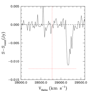
Figure 1.— Spectrum of the CSO 0035$+$227, with velocities displayed in the optical heliocentric convention. The systemic velocity of the optical galaxy is $v_{\rm sys}=(28,780\pm 600)$ km s${}^{-1}\,$: $v_{\rm sys}$ is marked with a vertical, dotted line; the horizontal, dotted line shows its 1$\sigma$ uncertainty. A complex absorption line, with $\tau_{\rm obs,peak}=0.0181\pm 0.0014$ and $\Delta V=(114\pm 10)$ km s${}^{-1}\,$, is detected about $v_{\rm sys}$.

III.4.2 HI absorption in 0941$-$080

In the spectrum of 0941$-$080, shown in Figure 2, we detected a broad, multi-peaked absorption feature. A Gaussian fit to the optical depth velocity profile yields a peak optical depth $\tau_{\rm obs,peak}=0.0022\pm 0.0002$, a line width $\Delta V=(215\pm 18)$ km s${}^{-1}\,$, and a peak velocity $v_{\rm peak}=(68156\pm 8)$ km s${}^{-1}\,$. The systemic velocity of the host galaxy, derived from the heliocentric redshift estimated from the optical spectrum of the source, $z=0.2281\pm 0.0013$ (de Vries et al. 2000, de Vries, private communication), is $v_{\rm sys}=(68353\pm 390)$ km s${}^{-1}\,$. The peak velocity of the absorption line is consistent with the systemic velocity of the galaxy at 1$\sigma$ confidence level. For the gas responsible for this associated absorption, we derived an HI column density $N_{\mathrm{HI}}$ =$(9.1\pm 1.0)\times 10^{19}$ cm${}^{-2}\,$, under the assumption that $C_{\rm f}=1$ and $T_{\rm s}=100$ K. This detection of HI absorption in the source is the first ever, and it was enabled by the improved observation setup (see Section III.2). Previous observations (Vermeulen et al. 2003) could only set upper limits to the optical depth of a putative absorption line (see Table A). The optical depth that we measured is consistent with the previously estimated upper limits.

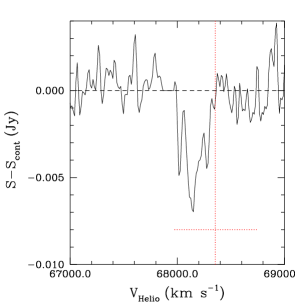
Figure 2.— Spectrum of the GPS/CSO galaxy 0941$-$080, with velocities displayed in the optical heliocentric convention. The systemic velocity of the optical galaxy is $v_{\rm sys}=(68,353\pm 390)$ km s${}^{-1}\,$: $v_{\rm sys}$ is marked with a vertical, dotted line; the horizontal, dotted line shows its 1$\sigma$ uncertainty. A broad, multi-peaked absorption feature with $\tau_{\rm obs,peak}=0.0022\pm 0.0002$ and $\Delta V=(215\pm 18)$ km s${}^{-1}\,$is detected about $v_{\rm sys}$.

IV. $N_{\mathrm{H}}$ - $N_{\mathrm{HI}}$ sample definition

By using our own data and those from the literature, we compiled the largest sample of GPS/CSOs that were targets of both X-ray and HI-absorption observations. The GPS/CSOs observed in the X-rays were all detected in this band, and they constitute a subsample of the GPS/CSOs observed in the HI band: therefore, the sample that we compiled consists of all the X-ray detected GPS/CSOs that were also observed in the HI band, i.e. 27 compact radio galaxies. This sample includes sources that were investigated in the X-ray band, either individually or in small samples, by different authors and with different instruments; it can be considered as the merger of two, partly overlapping, subsamples of sources that were selected for X-ray investigations with different criteria. The first subsample is a flux- and volume-limited sample of 17 GPS galaxies, with $F_{5\,\mathrm{G}Hz}>1$ Jy and $z<1$, extracted by Tengstrand et al. (2009) and Guainazzi et al. (2006) from the complete sample of GPS sources compiled by Stanghellini et al. (1998); these GPS galaxies are located at redshift $z=0.0773-0.99$, and have radio luminosities at $\nu=1.4$ GHz spanning the range $L_{\mathrm{1.4\,GHz}}=10^{25}-10^{28.4}$ W Hz^-1; 16 of them were morphologically classified as CSOs. The second subsample is a sample of 16 CSOs with known redshifts and estimated kinematic ages, compiled by Siemiginowska et al. (2016); these CSOs are located at redshift $z=0.0142-0.764$, and have radio luminosities at $\nu=1.4$ GHz spanning the range $L_{\mathrm{1.4\,GHz}}=10^{24}-10^{27.6}$ W Hz^-1; 15 of them were spectroscopically classified as GPS sources. The two subsamples have six sources in common. Overall, the 27 sources of the full sample are located at redshift $z=0.0142-0.99$, and they have moderate to high radio luminosities, $L_{\mathrm{1.4\,GHz}}=10^{24}-10^{28.4}$ W Hz^-1. Even though the sample is not complete and well-defined in terms of flux limit and volume, it is the largest sample of GPS/CSOs available to date for which both X-ray and HI observations were carried out. The main properties of the sources of this sample, including all the available HI and X-ray column density estimates, are summarized in Tables A and B.

In order to perform the $N_{\mathrm{H}}$ - $N_{\mathrm{HI}}$ correlation analysis, from the above sample of 27 GPS/CSOs we extracted the subsample of sources for which an estimate of both $N_{\mathrm{HI}}$ and $N_{\mathrm{H}}$ was available. By “estimate” we mean either a value or an upper/lower limit. The three sources 0026$+$346, 0710$+$439, and 2008$-$068 have no $N_{\mathrm{HI}}$ estimate (see Sections IV.1 and Table A), and the two sources 0116$+$319 and 1245$+$676 have no $N_{\mathrm{H}}$ estimate (see Sections IV.2 and Table B). Therefore, we were left with a subsample of 22 sources, that we refer to hereafter as the correlation sample.

The correlation sample spans the redshift range $z=0.0142-0.99$ and the 1.4 GHz luminosity range $L_{\mathrm{1.4\,GHz}}=10^{24.2}-10^{28.4}$ W Hz^-1. Table 2 lists the sources of the correlation sample (Column 1), their optical redshifts (Column 2), their radio spectral and morphological classification (Column 3), the estimates of $N_{\mathrm{HI}}$ (Column 4) and $N_{\mathrm{H}}$ (Column 5) that we used for the correlation analysis, the type of ($N_{\mathrm{H}}$,$N_{\mathrm{HI}}$) pair (Column 6), and the sample to which we associated each ($N_{\mathrm{H}}$,$N_{\mathrm{HI}}$) pair for the correlation analysis (Column 7), as described in Section IV.3. More details on the quantities reported in Table 2 and the criteria that we applied to select the column density estimates given in this table among all the available column density estimates, can be found in the Appendix.

Table 2Correlation Sample: Column Density Data Set, Pair Types, and Analysis Samples.

Source Name	$z_{\mathrm{opt}}$	GPS/CSO	$N_{\mathrm{HI}}$	$N_{\mathrm{H}}$	Pair Type	Sample
B1950			($10^{20}\frac{T_{\mathrm{s}}}{100\mathrm{\,K}}$ cm${}^{-2}\,$)	($10^{22}$ cm${}^{-2}\,$)
(1)	(2)	(3)	(4)	(5)	(6)	(7)
0019$-$000	0.305	GPS	$<1.5$	$<100$	UU	$E^{\prime}$, $E^{\prime\prime}$
0035$+$227	$0.096\pm 0.002$	CSO	$3.99\pm 0.49$	$1.4^{+0.8}_{-0.6}$	VV	$E^{\prime}$, $E^{\prime\prime}$
0108$+$388	0.66847	GPS,CSO	$80.5$	$47.5^{+12}_{-12}$	VV	$E^{\prime}$
			$80.5$	$>90$	VL	–
0428$+$205	0.219	GPS,CSO	3.45	$<0.69$	VU	$E^{\prime}$, $E^{\prime\prime}$
0500$+$019	0.58457	GPS,CSO	$6.2$	$0.5^{+0.18}_{-0.16}$	VV	$E^{\prime}$, $E^{\prime\prime}$
0941$-$080	0.2281$\pm$0.0013	GPS,CSO	$0.91\pm 0.10$	$<1.26$	VU	$E^{\prime}$, $E^{\prime\prime}$
1031$+$567	0.459	GPS,CSO	$<1.26$	$0.50\pm 0.18$	VU	$E^{\prime}$, $E^{\prime\prime}$
1117$+$146	0.362	GPS,CSO	$<0.63$	$<0.16$	UU	$E^{\prime}$, $E^{\prime\prime}$
1323$+$321	0.370	GPS,CSO	$0.71$	$0.12^{+0.06}_{-0.05}$	VV	$E^{\prime}$, $E^{\prime\prime}$
1345$+$125	0.12174	GPS,CSO	$6.2$	$4.8\pm 0.4$	VV	$E^{\prime}$, $E^{\prime\prime}$
			$6.2$	$2.543^{+0.636}_{-0.580}$	VV	$E^{\prime}$, $E^{\prime\prime}$
1358$+$624	0.431	GPS,CSO	$1.88$	$2.9^{+2}_{-1}$	VV	$E^{\prime}$, $E^{\prime\prime}$
1404$+$286	0.07658	GPS,CSO	$8.0$	$0.13^{+0.12}_{-0.10}$	VV	$E^{\prime}$
			$8.0$	$>90$	VL	–
1509$+$054	0.084	GPS,CSO	$<3.64$	$<0.23$	UU	$E^{\prime}$, $E^{\prime\prime}$
1607$+$268	0.473	GPS,CSO	$<1.6$	$<0.18$	UU	$E^{\prime}$, $E^{\prime\prime}$
1718$-$649	0.0142	GPS,CSO	1.477	$0.08\pm 0.07$	VV	$E^{\prime}$, $E^{\prime\prime}$
1843+356	0.764	GPS,CSO	$<10.4$	$0.8^{+0.9}_{-0.7}$	VU	$E^{\prime}$, $E^{\prime\prime}$
1934$-$638	0.18129	GPS,CSO	$0.06$	$0.08^{+0.07}_{-0.06}$	VV	$E^{\prime}$
			$0.06$	$>250$	VL	–
1943$+$546	0.263	GPS,CSO	$4.91$	$1.1\pm 0.7$	VV	$E^{\prime}$, $E^{\prime\prime}$
1946$+$708	0.101	GPS,CSO	$31.6$	$1.7^{+0.5}_{-0.4}$	VV	$E^{\prime}$
			$31.6$	$>280$	VL	–
2021$+$614	0.227	GPS,CSO	$<0.27$	$<1.02$	UU	$E^{\prime}$, $E^{\prime\prime}$
2128$+$048	0.99	GPS,CSO	$<2.08$	$<1.9$	UU	$E^{\prime}$, $E^{\prime\prime}$
2352$+$495	0.2379	GPS,CSO	2.84	$4^{+7}_{-3}$	VV	$E^{\prime}$, $E^{\prime\prime}$

IV.1. $N_{\mathrm{HI}}$ estimates

Detections of HI absorption features, and their corresponding $N_{\mathrm{HI}}$ values, were available for 14 out of the 22 sources of the correlation sample; $N_{\mathrm{HI}}$ upper limits could be estimated for the remaining eight sources.

We only used $N_{\mathrm{HI}}$ estimates derived from low angular resolution measurements, i.e. from measurements that were not able to spatially resolve the source; all our upper limits to $N_{\mathrm{HI}}$ are 3$\sigma$ limits. As mentioned in Sections II and III.4, the $N_{\mathrm{HI}}$ estimates depend on the value assumed for the ratio $T_{\mathrm{s}}/C_{\mathrm{f}}$. When an $N_{\mathrm{HI}}$ value drawn from the literature was estimated by the authors by assuming $T_{\mathrm{s}}/C_{\mathrm{f}}>100$ K (i.e., $T_{\mathrm{s}}>100$ K and $C_{\mathrm{f}}=1$), we rescaled it to an $N_{\mathrm{HI}}$ value computed with $T_{\mathrm{s}}/C_{\mathrm{f}}=100$ K. For the 12 sources with more than one $N_{\mathrm{HI}}$ estimate, we chose the most suitable estimate, according to the criteria described in Appendix A. The selected $N_{\mathrm{HI}}$ estimates are summarized in Table 2, Column 4; they are also listed with the corresponding references in Table A; we thoroughly comment on these data, as well as on on the properties of the full $N_{\mathrm{HI}}$ data set, in Appendix A.

IV.2. $N_{\mathrm{H}}$ estimates

As anticipated in Section II, the estimate of the column density of the X-ray absorbing gas located at the redshift of the source (i.e., the local absorber) depends on the X-ray emission model adopted to interpret the X-ray spectrum of the source, as well as on the assumed photoionization cross-section of the ISM. For a given abundance of chemical elements in the absorbing gas, the X-ray spectral modeling enables to estimate the equivalent hydrogen column density of the local absorber, $N_{\mathrm{H}}$ , i.e., the column density of hydrogen atoms, molecules, and ions toward the source, located at the source redshift (see Appendix B for details).

In the correlation sample, detections of intrinsic X-ray absorption, and corresponding values of $N_{\mathrm{H}}$, were available for nine out of 22 sources; upper limits to $N_{\mathrm{H}}$ were available for eight sources. For the remaining five sources, multiple exposures and ambiguity in the spectral modeling prevented us from selecting a single robust $N_{\mathrm{H}}$ value. In particular, for one source, we selected two significantly different $N_{\mathrm{H}}$ values corresponding to different observational epochs. For four of them, the ambiguity between a Compton-thin and a Compton-thick absorber in the model adopted for the interpretation of the X-ray spectrum of the source led to the availability of $N_{\mathrm{H}}$ estimates lower and greater than $\simeq 10^{24}$ cm${}^{-2}\,$, respectively; we considered both scenarios as plausible, and associated with each of these four sources either an $N_{\mathrm{H}}$ value (Compton-thin scenario) or a lower limit to $N_{\mathrm{H}}$ (Compton-thick scenario).

The $N_{\mathrm{H}}$ estimates that we used for our correlation analysis are summarized in Table 2, Column 5; they are also listed with the corresponding references in Table B; we thoroughly comment on these data, as well as on the properties of the full $N_{\mathrm{H}}$ data set, in Appendix B.

IV.3. $N_{\mathrm{H}}$ - $N_{\mathrm{HI}}$ sample

The correlation sample consists of 22 sources associated with ($N_{\mathrm{H}}$,$N_{\mathrm{HI}}$) pairs of estimates of four different types: pairs of values (hereafter referred to as VV pairs), pairs including a value and an upper limit (VU pairs), pairs of upper limits (UU pairs), and pairs including a value and a lower limit (VL pairs). Specifically, the sample includes four sources unambiguously associated with VU pairs, six with UU pairs, and eight with VV pairs. The sample also includes four sources whose X-ray absorber may be either Compton-thin or Compton-thick (see Section IV.2): each of them is associated with either a $VV$ pair or a $VL$ pair. The types of ($N_{\mathrm{H}}$,$N_{\mathrm{HI}}$) pairs associated with the sources of the correlation sample are listed in Table 2, Column 6.

In order to deal with the four ambiguous Compton-thin/Compton-thick sources, we considered two limiting cases in our correlation study. In the first case, we assumed these four sources to be all Compton-thin, and hence we associated them with VV pairs. This choice yielded a correlation sample composed of 12 sources with ($N_{\mathrm{H}}$,$N_{\mathrm{HI}}$) pairs of values (VV pairs) and 10 sources with ($N_{\mathrm{H}}$,$N_{\mathrm{HI}}$) pairs including upper limits (either VU or UU pairs), for a total of 22 sources with 23 ($N_{\mathrm{H}}$,$N_{\mathrm{HI}}$) pairs of estimates of either the VV, the VU, or UU type; hereafter, this sample is referred to as the estimate sample $E^{\prime}$. The data in sample $E^{\prime}$ have only one type of censoring (i.e., the sample pairs include only values and upper limits; there is no mix of upper and lower limits).

In the second case, we assumed the above four sources to be all Compton-thick, and associated them with the corresponding VL pairs. This left us with a correlation sample composed of three main subsamples: a subsample of eight sources with ($N_{\mathrm{H}}$,$N_{\mathrm{HI}}$) VV pairs, a subsample of 10 sources including upper limits (either VU or UU pairs), and a subsample of four sources including lower limits (VL pairs). However, because of difficulties in performing the correlation analysis on samples including data with two types of censoring (i.e., both upper and lower limits; see Section V for details), we chose to drop the four VL pairs from the correlation sample. The reason why we dropped this subsample of pairs is that this is the smaller of the two subsamples of censored data pairs. Dropping the subsample that includes the VU and UU pairs would have lowered the total number of sources. Our choice left us with a sample including eight sources with ($N_{\mathrm{H}}$,$N_{\mathrm{HI}}$) VV pairs, and 10 sources with ($N_{\mathrm{H}}$,$N_{\mathrm{HI}}$) pairs of estimates of either the VU or the UU type, for a total of 18 sources with 19 ($N_{\mathrm{H}}$,$N_{\mathrm{HI}}$) pairs of estimates of either the VV, the VU, or the UU type; hereafter, this sample is referred to as the estimate sample $E^{\prime\prime}$. By construction, the data in sample $E^{\prime\prime}$ have only one type of censoring.

V. Correlation analysis

We performed the correlation analysis on both the estimate samples, $E^{\prime}$ and $E^{\prime\prime}$, defined in Section IV.3. The results of this analysis are reported in Table 3, and are discussed below. Figure 3 displays the ($N_{\mathrm{H}}$,$N_{\mathrm{HI}}$) data for these two samples, as well as the corresponding linear regression lines, to guide the eye.

Before discussing these results, we emphasize that correlating $N_{\mathrm{H}}$ with $N_{\mathrm{HI}}$ is interesting from the point of view of the physics of the sources, although the estimate of $N_{\mathrm{HI}}$ is a combination of the measurement of $\tau_{\rm obs}$ and the assumption on $T_{\rm s}/C_{\rm f}$ ($N_{\mathrm{HI}}$$\propto\tau_{\rm obs}\times T_{\rm s}/C_{\rm f}$; see Equation 3).

Figure 3.— Radio column densities ($N_{\mathrm{HI}}$) as a function of X-ray column densities ($N_{\mathrm{H}}$) for the estimate samples, $E^{\prime}$ (left) and $E^{\prime\prime}$ (right). The solid symbols show the ($N_{\mathrm{H}}$,$N_{\mathrm{HI}}$) measurements with 1$\sigma$ error bars on $N_{\mathrm{H}}$. Arrows represent upper limits. Lower limits to $N_{\mathrm{H}}$ corresponding to possibly Compton-thick sources are shown in the plot on the right as open triangles, although they were not included in the correlation analysis. Labels show a shortened version of the source names reported in Table A. $N_{\mathrm{HI}}$ was computed by assuming $T_{\mathrm{s}}=100$ K and $C_{\mathrm{f}}=1$. Solid line: Akritas-Thiel-Sen regression line, to guide the eye ($\log_{10}$$N_{\mathrm{HI}}$$=a+b\log_{10}$$N_{\mathrm{H}}$; see Table 3); dotted line: Schmitt’s regression line, for a bin number of 10 (see Section V for details); dashed line: bisector of the $N_{\mathrm{H}}$-$N_{\mathrm{HI}}$ plane.

Table 3Correlation and Regression Analysis for the Estimate Samples, $E^{\prime}$ and $E^{\prime\prime}$, by means of Survival Analysis Techniques.

Sample	Ndata	Generalized Kendall		Generalized Spearman		Schmitt’s Linear Regression		Akritas-Theil-Sen Linear Regression
	(Nsources)	$z$	$P$	$\rho$	$P$	Slope (b)	Intercept (a)	Slope (b)	Intercept (a)
$E^{\prime}$	23 (22)	3.044	0.0023	0.679	0.0014	0.820	2.42	0.467	10.3
$E^{\prime\prime}$	19 (18)	2.615	0.0089	0.667	0.0046	0.469	10.0	0.345	13.0

In the estimate samples, we investigated the correlation by means of survival analysis techniques. In particular, we made use of the software package ASURV Rev. $1.3$ (LaValley et al. 1992), which implements the methods for bivariate problems presented in Isobe et al. (1986). The generalized Kendall’s correlation analysis applied to samples $E^{\prime}$ and $E^{\prime\prime}$ shows that the data are significantly correlated: the probability of no correlation being true is $P=2.3\times 10^{-3}$ for sample $E^{\prime}$, and $P=8.9\times 10^{-3}$ for sample $E^{\prime\prime}$. The generalized Spearman’s correlation analysis applied to the same samples confirms the above results: $P=1.4\times 10^{-3}$ for sample $E^{\prime}$, and $P=4.6\times 10^{-3}$ for sample $E^{\prime\prime}$. The reason why the significance of the correlation for sample $E^{\prime\prime}$ is slightly lower than for sample $E^{\prime}$ is that sample $E^{\prime\prime}$ does not include, among other sources, the two targets characterized by extreme ($N_{\mathrm{H}}$,$N_{\mathrm{HI}}$) values.

In order to describe the relationship between $N_{\mathrm{H}}$ and $N_{\mathrm{HI}}$, we performed a regression analysis with $N_{\mathrm{HI}}$ as the dependent variable. The selection criteria of the correlation sample (see Section IV) do not introduce any bias in this sample; therefore, either $N_{\mathrm{HI}}$ or $N_{\mathrm{H}}$ can formally play the role of the dependent variable. Our choice of $N_{\mathrm{HI}}$ as the dependent variable is motivated by the fact that, from a physical perspective, in a given gas distribution, the mass fraction of neutral, atomic gas depends upon the total (i.e., molecular, atomic, and ionized) gas mass through the physical properties of the gas. As a consequence, for the same gaseous structure, the contribution of $N_{\mathrm{HI}}$ to $N_{\mathrm{H}}$ depends on the physical conditions and on the geometrical distribution of the gas (i.e., temperature and covering factor).

According to the generalized Kendall’s and Spearman’s tests, we could fit a linear relation to the estimate samples $E^{\prime}$ and $E^{\prime\prime}$: $\log_{10}$$N_{\mathrm{HI}}$ $=a+b$ $\log_{10}$$N_{\mathrm{H}}$ . We first performed a linear fit to the data by means of the ASURV Schmitt’s linear regression. This method requires a binning of the data set. For sample $E^{\prime}$, by varying the number of data bins from 3 to 15, we obtained slopes in the range $b=0.51-0.99$; for sample $E^{\prime\prime}$, by varying the number of data bins from 3 to 15, we obtained slopes in the range $b=0.41-0.57$.

For both $E^{\prime}$ and $E^{\prime\prime}$, we show the representative results for the case of 10 bins (dotted lines in Figure 3). Because the results of Schmitt’s regression analysis are sensitive to the bin size for small data sets, we performed an additional estimation of the slope with the Akritas-Theil-Sen estimator (e.g., Akritas et al. 1995; Feigelson & Babu 2012), that is implemented in the function cenken in the CRAN package NADA within the R statistical software environment. With this method, we found regression-line slopes $b=0.47$ and $b=0.35$ for samples $E^{\prime}$ and $E^{\prime\prime}$, respectively (solid lines in Figure 3). We adopted the slopes derived with the Akritas-Theil-Sen estimator as our trustworthy estimates because of their independence of the binning of the data set.

We note that the Akritas-Theil-Sen method applied to samples $E^{\prime}$ and $E^{\prime\prime}$ after switching the roles of the variables (i.e. by assuming $N_{\mathrm{HI}}$ as the independent variable) returned slopes $B=0.76$ and $B=1.10$, respectively, for the regression line $\log_{10}$$N_{\mathrm{H}}$ $=A+B$ $\log_{10}$$N_{\mathrm{HI}}$ , in agreement with our previous results (Ostorero et al. 2009, 2010).

VI. Discussion

With the survival analysis methods described in Section V, we found $N_{\mathrm{H}}$ and $N_{\mathrm{HI}}$ in samples $E^{\prime}$ and $E^{\prime\prime}$ to be significantly correlated and to be related to each other through the relationship $N_{\mathrm{HI}}$$\propto$$N_{\mathrm{H}}$^b, with $b=0.47$ and $b=0.35$. Neither the uncertainties on the regression parameters nor the goodness of the fit could be evaluated. However, a visual inspection of this data set suggests a dispersion larger than the typical uncertainties on $N_{\mathrm{HI}}$ (see Figure 3).

This fact is supported by the regression analysis of the subsamples that we drew from $E^{\prime}$ and $E^{\prime\prime}$ by selecting the detections only. These two subsamples, hereafter referred to as detection samples $D^{\prime}$ and $D^{\prime\prime}$, respectively, display a significant $N_{\mathrm{H}}$ - $N_{\mathrm{HI}}$ correlation according to both Pearson’s and Kendall’s correlation analysis. However, the best-fit linear relation turns out not to be a good description of the data ($\chi^{2}_{\mathrm{red}}\sim 10$): the dispersion of the data is clearly larger than the typical uncertainties.

This evidence suggests that the observed $N_{\mathrm{H}}$ - $N_{\mathrm{HI}}$ relation is the two-dimensional projection of a multi-dimensional relation, where $T_{\rm s}/C_{\rm f}$ is a variable rather than a parameter. In fact, as we show below, $T_{\rm s}/C_{\rm f}$ is the most relevant additional variable in the $N_{\mathrm{H}}$ - $N_{\mathrm{HI}}$ relation. There are only two other possible variables; however, they either have a modest impact or, ultimately, depend on $T_{\rm s}$: (i) the abundance of chemical elements that enters the photoionization cross-section of the X-ray absorbing gas, ultimately affecting the $N_{\mathrm{H}}$ estimates in the X-ray spectral fitting; and (ii) the amount of ionized and molecular hydrogen, HII and H₂.

As for item (i), typical cross-sections adopted in the spectral analysis are based on either solar or ISM abundances. These different assumptions lead to variations of the cross-section by a factor of a few (e.g., Ride & Walker 1977; Wilms et al. 2000), implying corresponding variations of the $N_{\mathrm{H}}$ estimates by a factor of a few. This variation is comparable to the average $N_{\mathrm{H}}$ uncertainty.

As for item (ii), the abundance of HII and H₂ is an unknown that, in principle, can contribute both to the $N_{\mathrm{H}}$ - $N_{\mathrm{HI}}$ offset and to the spread. This abundance is ultimately set by the kinetic temperature of the gas, $T_{\rm k}$. If all the sources were characterized by a similar kinetic temperature of the absorber, the fractions of HII and/or H₂ would be comparable in different sources and would only contribute to the offset. On the other hand, if the kinetic temperature were significantly different in different sources, the abundance of HII and H₂ would also contribute to the spread, and $N_{\mathrm{H}}$ and $N_{\mathrm{HI}}$ might even be uncorrelated in the case of extreme temperature fluctuations. However, we do find a correlation between $N_{\mathrm{H}}$ and $N_{\mathrm{HI}}$: we can thus exclude extreme fluctuations in the kinetic temperature, $T_{\rm k}$.

Similarly, the ratio $T_{\rm s}/C_{\rm f}$ might also significantly fluctuate from source to source; for example, it is seen to vary by a factor of at least $\sim 170$ in damped Ly-$\alpha$ systems, where HI column densities are known (Curran et al. 2013). Clearly, extreme fluctuations of $T_{\rm s}/C_{\rm f}$ from source to source might also erase the $N_{\mathrm{H}}$ - $N_{\mathrm{HI}}$ correlation. As in the case of $T_{\rm k}$, the correlation we found excludes extreme fluctuations in $T_{\rm s}/C_{\rm f}$. Because $T_{\rm k}$ and $T_{\rm s}$ are related to each other, we can ultimately ascribe the correlation spread to fluctuations of $T_{\rm s}/C_{\rm f}$ about the assumed value.

To sum up, for a given source, the $N_{\mathrm{HI}}$ estimate from a spatially unresolved measurement of $\tau_{\rm obs}$ must assume a value for the ratio $T_{\rm s}/C_{\rm f}$; typically, $T_{\rm s}/C_{\rm f}$=100 K is assumed. A different assumption about $T_{\rm s}/C_{\rm f}$ clearly leads to a different $N_{\mathrm{H}}$ - $N_{\mathrm{HI}}$ offset. When we look for a correlation between X-ray and radio absorption in a sample of sources, we must also assume a $T_{\rm s}/C_{\rm f}$ ratio for each source. The simplest assumption is to assign the same ratio to all the sources. A posteriori, this assumption appears to be reasonable because we do find a correlation. However, this correlation shows a non-null spread, suggesting that each individual source might actually have a $T_{\rm s}/C_{\rm f}$ ratio slightly different from the value assumed for the entire sample. By estimating the spread, one can, in principle, estimate the fluctuations of the $T_{\rm s}/C_{\rm f}$ ratio of the individual sources about the value assumed for the entire sample. As a proof of concept, we estimate the spread of the detection samples $D^{\prime}$ and $D^{\prime\prime}$ in Section VI.1.

VI.1. Quantifying the spread of the $N_{\mathrm{H}}$ - $N_{\mathrm{HI}}$ correlation

In order to simultaneously derive the correlation parameters of the $N_{\mathrm{H}}$ - $N_{\mathrm{HI}}$ relation and quantify, for a given $N_{\mathrm{H}}$, the intrinsic scatter of $N_{\mathrm{HI}}$ that might be due to the fluctuation of the ratio $T_{\rm s}/C_{\rm f}$ of the individual sources about a mean value, it is appropriate to resort to a Bayesian analysis. As a proof of concept, we performed a Bayesian analysis of the detection samples $D^{\prime}$ and $D^{\prime\prime}$. We made use of the code APEMoST, which was developed by J. Buchner and M. Gruberbauer (Gruberbauer et al. 2009) and is suitable for non-censored data sets. A more sophisticated code, able to perform the Bayesian analysis on samples that include double-censored data (as our samples $E^{\prime}$ and $E^{\prime\prime}$), could be constructed based on the model developed by Kelly (2007); however, this implementation is beyond the scope of the present paper.

Although samples $D^{\prime}$ and $D^{\prime\prime}$ are biased, because they do not include non-detections, the results presented below are useful to illustrate how the intrinsic spread of the $N_{\mathrm{H}}$ - $N_{\mathrm{HI}}$ relation can be quantified and interpreted. An additional advantage of the Bayesian analysis over the frequentist analysis is the possibility to take the uncertainties on both variables into account, even when the uncertainties are asymmetric.

Our data set is $DS$={$\log_{10}$$N_{\mathrm{H}}$^k, $\log_{10}$$N_{\mathrm{HI}}$^k, $\mathbf{S}^{k}$}, where $\mathbf{S}^{k}=\{\sigma^{k}_{+},\sigma^{k}_{-},\epsilon^{k}_{+},\epsilon^{k}_{-}\}$ is the vector of the upper and lower uncertainties on the $k$-th measures $N_{\mathrm{H}}$^k and $N_{\mathrm{HI}}$^k. The uncertainties on the $N_{\mathrm{HI}}$ values, for a given $T_{\rm s}/C_{\rm f}$, are available for two measurements only: the relative uncertainties are equal to 12% and 14%, respectively. Assuming that the remaining $N_{\mathrm{HI}}$ measurements are affected by comparable uncertainties, for the purpose of the Bayesian analysis only, to each of them we associated a conservative, relative uncertainty of 15%. Because the uncertainties on $N_{\mathrm{HI}}$ are much smaller than those on $N_{\mathrm{H}}$, all the $N_{\mathrm{HI}}$ uncertainties have negligible effects on our results.

Given our data set $DS$, we determined the multi-dimensional probability density function (PDF) of the parameters $\theta=\{a,b,\sigma_{\rm int,NHI}\}$, where $a$ and $b$ are the parameters of the correlation (i.e., our model $M$):

$$\log_{10}N_{\rm HI}=a+b\log_{10}N_{\rm H}\pm\sigma_{\rm int,NHI},$$ (5)

and $\sigma_{\rm int,NHI}$ is the intrinsic spread of the dependent variable.

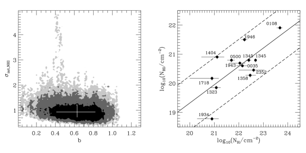
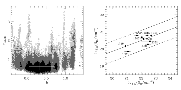
Figure 4.— Bayesian analysis applied to sample $D^{\prime}$ (top) and $D^{\prime\prime}$ (bottom), with $N_{\mathrm{H}}$ as the independent variable and $N_{\mathrm{HI}}$ as dependent variable. The left panels show the marginalized PDFs of the parameters $b$ and $\sigma_{\rm int,NHI}$. Black, gray, and light-gray shaded regions correspond to the 68.3, 95.4, and 99.7% confidence levels, respectively. The crosses show the median values and their marginalized 1$\sigma$ uncertainty. The right panels show the $N_{\mathrm{H}}$ - $N_{\mathrm{HI}}$ correlation: the solid symbols show the ($N_{\mathrm{H}}$,$N_{\mathrm{HI}}$) measurements with their 1$\sigma$ error bars (relative uncertainties of 15% were assumed for the $N_{\mathrm{HI}}$ values whose uncertainty was not available in the literature; see text for details); the solid, straight line is the $N_{\mathrm{H}}$ - $N_{\mathrm{HI}}$ relation $\log_{10}$$N_{\mathrm{HI}}$$=a+b\log_{10}$$N_{\mathrm{H}}$; the dashed lines show the $\pm\sigma_{\rm int,NHI}$ standard deviation of the relation; the parameters $a$, $b$, and $\sigma_{\rm int,NHI}$ are listed in Table 4.

In our analysis with APEMoST, we assumed independent flat priors for parameters $a$ and $b$. For the internal dispersion $\sigma_{\rm int,NHI}$, which is a positive parameter, we assumed

$$p(\sigma_{\rm int,NHI}|M)={\mu^{r}\over\Gamma(r)}x^{r-1}\exp(-\mu x)\,,$$ (6)

where $x=1/\sigma_{\rm int,NHI}^{2}$, and $\Gamma(r)$ is the Euler gamma function. This PDF describes a variate with mean $r/\mu$, and variance $r/\mu^{2}$. We set $r=\mu=10^{-5}$ to assure an almost flat prior.

We used $2\times 10^{6}$ MCMC iterations to guarantee a fairly complete sampling of the parameter space. The boundaries of the parameter space were set to $[-1000,1000]$ for the $a$ and $b$ parameters, and to $[0.01,1000]$ for the $\sigma_{\rm int,NHI}$ parameter. The initial seed of the random number generator was set with the bash command GSL_RANDOM_SEED=$RANDOM.

The results of this analysis are reported in Table 4, and displayed in Figure 4.

Table 4Bayesian Analysis of the Detection Samples, $D^{\prime}$ and $D^{\prime\prime}$: Median Fit Parameters of the $N_{\mathrm{H}}$ - $N_{\mathrm{HI}}$ Relation.

Sample	Ndata (Nsources)	$a$	$b$	$\sigma_{\rm int,NHI}$
$D^{\prime}$	13 (12)	$6.7^{+4.8}_{-4.2}$	$0.63^{+0.19}_{-0.22}$	$0.92^{+0.30}_{-0.21}$
$D^{\prime\prime}$	9 (8)	$13.5^{+5.8}_{-8.4}$	$0.32^{+0.38}_{-0.27}$	$0.59^{+0.38}_{-0.18}$

Our analysis applied to sample $D^{\prime}$ shows that, for any given value of $\log_{10}$$N_{\mathrm{H}}$, $\log_{10}$$N_{\mathrm{HI}}$ takes the value $\log_{10}$$N_{\mathrm{HI}}$ $=a+b\log_{10}$$N_{\mathrm{H}}$ $\pm\sigma_{\rm int,NHI}$ (with $a=6.7^{+4.8}_{-4.2}$, $b=0.63^{+0.19}_{-0.22}$, and $\sigma_{\rm int,NHI}=0.92^{+0.30}_{-0.21}$), with a 68% probability; this value of the intrinsic spread implies that, for any given $N_{\mathrm{H}}$, the corresponding $N_{\mathrm{HI}}$ falls within a factor of $\simeq 8$ from the mean relation at the 68% confidence level.

As for the smaller sample $D^{\prime\prime}$, our analysis yielded $b=0.32^{+0.38}_{-0.27}$ and a smaller intrinsic spread, $\sigma_{\rm int,NHI}=0.59^{+0.38}_{-0.18}$, which implies that, for any given $N_{\mathrm{H}}$, the corresponding $N_{\mathrm{HI}}$ falls within a factor of $\simeq 4$ from the mean relation with 68% probability. Because $D^{\prime\prime}$ was obtained from $D^{\prime}$ by removing the four ambiguous Compton-thin/thick sources, this means that those sources were responsible for the larger spread on $N_{\mathrm{HI}}$ that we found for sample $D^{\prime}$ (compare the top and bottom panels on the right-hand-side of Figure 4).

Overall, for the detection samples $D^{\prime}$ and $D^{\prime\prime}$, the value of the regression line’s slope is $b\simeq 0.3-0.6$, consistent with the results of the regression analyses presented in Section V for the estimate samples $E^{\prime}$ and $E^{\prime\prime}$.

We discuss the possible implications of our exercise on the evaluation of the spread that might be due to $T_{\rm s}/C_{\rm f}$ fluctuations in Section VI.2.

VI.2. Implications of the $N_{\mathrm{H}}$ - $N_{\mathrm{HI}}$ correlation and its spread

The $N_{\mathrm{H}}$ - $N_{\mathrm{HI}}$ correlation that we found in Section V suggests a physical connection between the X-ray and HI absorbers: the gas responsible for the X-ray obscuration and the HI absorption in compact radio galaxies may be part of the same, possibly unsettled, gaseous structure that extends over scales of a few hundred parsecs.

This scenario, also supported by recent X-ray and HI observations of a composite sample of compact radio sources (Glowacki et al. 2017), is corroborated by the X-ray absorption properties of the full X-ray emitting GPS/CSO sample: the mean total hydrogen column density of this sample (see Table B) varies from $N_{\mathrm{H}}$ $\simeq(0.8-1)\times 10^{22}$ cm^-2 ($\sigma_{N_{H}}\simeq 0.2-0.3$ dex) to $N_{\mathrm{H}}$ $\simeq 3\times 10^{22}$ cm^-2 ($\sigma_{N_{H}}\simeq 1$ dex), depending on whether absorbers that are not unambiguously Compton-thin are considered to be Compton-thin or Compton-thick sources, respectively. These values are consistent with a picture where the absorption of the X-rays from compact radio galaxies of the GPS/CSO type is comparable to the X-ray absorption in the extended FR-I and the unobscured FR-II radio galaxies. Together with the $N_{\mathrm{H}}$ - $N_{\mathrm{HI}}$ correlation, which points toward a physical connection between the X-ray and radio absorbers, this evidence suggests that, in GPS/CSOs, the X-ray absorbing gas is located on scales larger than those of the parsec-scale, dusty tori typically invoked in AGN unification schemes. Such a scenario would imply that either “standard” dusty tori are not present in compact radio galaxies, or that the dominant contribution to the X-ray emission of GPS/CSOs does not originate in the accretion disc, but rather in the larger-scale jet/lobe components.

Even though the $N_{\mathrm{H}}$ - $N_{\mathrm{HI}}$ correlation is statistically significant, the correlated data set is affected by a large intrinsic spread. For the detection samples, we could quantify the spread by means of a Bayesian analysis (Section VI.1). This spread could potentially provide us with interesting constraints on the properties of the neutral hydrogen in the ISM of the host galaxies of compact radio sources.

The $N_{\mathrm{H}}$ - $N_{\mathrm{HI}}$ correlation that we found actually reflects a correlation between $N_{\mathrm{H}}$ and $\tau_{\rm obs}$. Indeed, $N_{\mathrm{HI}}$$\propto T_{\rm s}/C_{\rm f}\times\tau_{\rm obs}$, with $\tau_{\rm obs}\equiv\int{\tau_{\rm obs}(v)\,{\mathrm{d}}v}$ (see Equation (3)); in our case, the only observable is the velocity-integrated optical depth of the absorption line, $\tau_{\rm obs}$, because we only considered spatially unresolved observations ($C_{\rm f}=1$) and we assumed $T_{\rm s}=100$ K for the absorbing gas, so we obtained a ratio of $T_{\rm s}/C_{\rm f}=100$ K for all the sources.

However, the ratio $T_{\rm s}/C_{\rm f}$ is seen to vary by a factor of at least $\sim 170$ (from 60 K to 9950 K) in damped Ly-$\alpha$ systems, where $N_{\mathrm{HI}}$ column densities are known (Curran et al. 2013); furthermore, the analysis of the compact quasar PKS 1549$-$79 suggests that $T_{\rm s}>3000$ K in this source (Holt et al. 2006); therefore, the assumption of a common value $T_{\rm s}/C_{\rm f}=100$ K for the sources analized here is not well-justified.

If $N_{\mathrm{H}}$ and $N_{\mathrm{HI}}$ were intrinsically tightly correlated, the assumption of a constant $T_{\rm s}/C_{\rm f}$ would be responsible for the $N_{\mathrm{HI}}$ spread that we measured. As an example, when the intrinsic spread of $N_{\mathrm{HI}}$ is $\sigma_{\rm int,NHI}=0.92$ (as for sample $D^{\prime}$, see Table 4), for any given $N_{\mathrm{H}}$, the corresponding observed $N_{\mathrm{HI}}$ falls within a factor of $\simeq 8$ from the mean relation. However, if the correct value of $N_{\mathrm{HI}}$ actually lies on the mean relation, its observed deviation derives from the incorrect assumption $T_{\rm s}/C_{\rm f}=100$ K and the factor of $\simeq 8$ has to be associated to the fluctuations of $T_{\rm s}/C_{\rm f}$ about 100 K; in other words, this ratio is expected to be in the range $T_{\rm s}/C_{\rm f}=12-832$ K, at the 68% confidence level.

Therefore, we can, in principle, use our Bayesian result to forecast the true $N_{\mathrm{HI}}$ value and constrain the $T_{\rm s}/C_{\rm f}$ fluctuation: for any given $N_{\mathrm{H}}$, the corresponding true $N_{\mathrm{HI}}$ value lies on the mean relation; by comparing the true value with the observed value, we can infer the deviation of the $T_{\rm s}/C_{\rm f}$ value from the assumed 100 K. This argument is sketched in Figure 5.

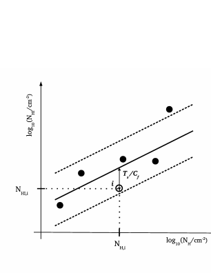
Figure 5.— If a true $N_{\mathrm{H}}$ - $N_{\mathrm{HI}}$ correlation exists (solid line), the observation of a source $i$ off the correlation is due to a deviation of $T_{\rm s}/C_{\rm f}$ from the value assumed for the entire $N_{\mathrm{HI}}$ sample. Specifically, a source appears below the mean relation when the value of $T_{\rm s}/C_{\rm f}$ assumed for the sample is too low: the value of $T_{\rm s}/C_{\rm f}$ that is appropriate for source $i$ and brings it back on the mean relation is proportionally larger, as indicated by the arrow.

In our sample, the HI observations do not spatially resolve the source and the HI is observed only in absorption. Therefore, $T_{\rm s}$ and $C_{\rm f}$ cannot be disentangled, and the estimate of $T_{\rm s}/C_{\rm f}$ does not enable to constrain the spin temperature of the gas. On the other hand, if HI measures of a sufficiently large sample of sources were based on high angular resolution observations, constraining $T_{\rm s}$ would, in principle, be possible. Indeed, this kind of observation enables to locate the HI absorber; the absorption profiles are derived only for the source region covered by the absorber, and the condition $C_{\rm f}=1$ is readily justified. Moreover, Equations (1) and (3) are more suitable for resolved observations; those equations hold under the assumption that the source is homogeneous, as appropriate when the source fraction considered for the evaluation of $N_{\mathrm{HI}}$ is small.

In conclusion, if a sample of resolved sources confirmed a correlation between $N_{\mathrm{H}}$ and $N_{\mathrm{HI}}$ , the deviation between the data-point of an individual source and the mean relation would return an estimate of the deviation of the spin temperature $T_{\rm s}$ of the HI in that source from the $T_{\rm s}$ assumed for the $N_{\mathrm{HI}}$ estimate of the entire sample.

VII. Conclusions

We performed spatially unresolved HI absorption observations of a sample of X-ray emitting GPS/CSO galaxies with the WSRT, in order to improve the statistics of the $N_{\mathrm{H}}$ - $N_{\mathrm{HI}}$ correlation sample and thoroughly investigate the possible connection between X-ray and radio absorbers in compact radio galaxies.

We confirmed the significant positive correlation between $N_{\mathrm{H}}$ and $N_{\mathrm{HI}}$ found by Ostorero et al. (2010), which implies that GPS/CSOs with increasingly large X-ray absorption have an increasingly larger probability of being detected in HI absorption observations. More interestingly, this correlation suggests that the gas responsible for the X-ray and radio absorption may be part of the same, possibly unsettled, hundred-parsec scale structure.

For the full, censored data set, the Akritas-Theil-Sen regression analysis yields $N_{\mathrm{HI}}$$\propto$$N_{\mathrm{H}}$^b, with $b=0.47$ and $b=0.35$, depending on the subsample. The correlation displays a large intrinsic spread, which may indicate that the $N_{\mathrm{H}}$ - $N_{\mathrm{HI}}$ relation is not a one-to-one relation; additional variables are involved in the correlation and generate the intrinsic spread of the data set.

The estimate of $N_{\mathrm{HI}}$ relies on the assumed value of the ratio $T_{\rm s}/C_{\rm f}$ between the spin temperature of the absorbing gas and its covering factor. We suggested that the additional variable mostly responsible for the $N_{\mathrm{HI}}$ spread around the mean $N_{\mathrm{H}}$ - $N_{\mathrm{HI}}$ correlation is the source-to-source fluctuation of $T_{\rm s}/C_{\rm f}$ with respect to the value assumed for the entire sample. An estimate of the $N_{\mathrm{HI}}$ spread at fixed $N_{\mathrm{H}}$, i.e. $\sigma_{\rm int,NHI}$, can be obtained through a Bayesian analysis. As a proof of concept, we performed this analysis on two uncensored subsamples only. For the larger subsample, we found $\sigma_{\rm int,NHI}=0.92$, implying that, for any given $N_{\mathrm{H}}$, $T_{\rm s}/C_{\rm f}$ is expected to fall within a factor of $\simeq 8$, at the 68% confidence level, from the value $T_{\rm s}/C_{\rm f}=$ 100 K assumed for the whole sample. If the existence of an $N_{\mathrm{H}}$ - $N_{\mathrm{HI}}$ correlation were confirmed by high angular resolution observations of large enough samples, we could, in principle, disentangle $T_{\rm s}$ from $C_{\rm f}$ and constrain the deviation of the gas spin temperature, $T_{\rm s}$, from the assumed value. This result would provide an unprecedented piece of information on the physical properties of the HI absorbing gas.

Appendix A $N_{\mathrm{HI}}$ estimates

Table A lists the names of the 27 GPS/CSOs of the sample described in Section IV (Column 1), their redshift (Column 2), their radio spectral and morphological classification as GPS and/or CSO (Column 3), their $N_{\mathrm{HI}}$ estimate (Column 4), the type (low/high-angular resolution) of HI absorption observation from which the $N_{\mathrm{HI}}$ estimate was derived, with possible estimates of the covering factor of the absorbing gas (Column 5), the label associated with the absorption line(s) the $N_{\mathrm{HI}}$ estimate refers to (Column 6), the width of the absorption line (Column 7) and its peak optical depth (Column 8), the instrument used for the HI observation (Column 9), and the reference for the HI measurement (Column 10).

In this table, the 22 sources of the correlation sample and the corresponding $N_{\mathrm{HI}}$ estimates that we used for the correlation analysis are highlighted with boldface fonts. The criteria that we adopted to select the column density estimates highlighted in Column 4 among all the available estimates are described below.

For three sources of the correlation sample, both low angular resolution HI absorption measurements (unable to spatially resolve the source) and high angular resolution HI absorption measurements (able to spatially resolve the source) were available; in Table A, Column 5, we denoted them by “U” (unresolved) and “R” (resolved), respectively. For self-consistency of the correlation analysis, we discarded the “R” measurements and made use of the “U” measurements only. For sources that were not detected, 3$\sigma$ upper limits to $N_{\mathrm{HI}}$ were chosen for the analysis.

After applying these criteria, our sample of 22 sources turned out to be composed of two subsamples, in terms of number of available $N_{\mathrm{HI}}$ estimates. For 10 out of 22 sources, only one unresolved $N_{\mathrm{HI}}$ estimate was available: we took this value for our correlation data set. Conversely, more than one unresolved $N_{\mathrm{HI}}$ estimate was available for any of the remaining 12 sources: for the purpose of our correlation analysis, we proceeded as follows.

For 5 out of 12 sources, two spectral features (marked with “I” and “II”, respectively, in Table A, Column 6) were detected in the HI absorption spectra. In three of them, $N_{\mathrm{HI}}$ was available for each absorption line, but not for the full spectrum: we associated with each of these sources a value of $N_{\mathrm{HI}}$ estimated as the sum of the $N_{\mathrm{HI}}$ values of each spectral line (this is the value reported in Table 2). In the other two sources, besides the $N_{\mathrm{HI}}$ of each line, also the total $N_{\mathrm{HI}}$ (marked with “tot.” in Table A, Column 6) was available: we associated the latter $N_{\mathrm{HI}}$ value with these sources.

For 7 out of 12 sources, either one or no absorption features were detected in different observations. When multiple $N_{\mathrm{HI}}$ values were available for a given source, we chose the most recent result. When an $N_{\mathrm{HI}}$ value and one or more upper limits to $N_{\mathrm{HI}}$ were available, we chose the $N_{\mathrm{HI}}$ value. When different 3$\sigma$ upper limits to $N_{\mathrm{HI}}$ were available, we chose the most stringent one.

Table 5HI Column Densities and Spectral Parameters.

Source Name	$z_{\mathrm{opt}}$	GPS/CSO	$N_{\mathrm{HI}}$	Res./Unres.	Line nr.	$\Delta V$	$\tau_{\mathrm{peak}}$	Instrument	References
B1950			($10^{20}\frac{T_{\mathrm{s}}}{100\mathrm{\,K}}$ cm${}^{-2}\,$)	(and $C_{\mathrm{f}}$)		(km s${}^{-1}\,$)	($10^{-2}$)
(1)	(2)	(3)	(4)	(5)	(6)	(7)	(8)	(9)	(10)
0019$-$000	0.305	GPS	$\cdots$	U	$\cdots$	$\cdots$	$\cdots$	WSRT	P03
			$\mathbf{<1.5}$	U	$\cdots$	$\cdots$	$<0.84$	WSRT	($\star$)
0026$+$346	0.517	GPS,CSO	$\cdots$	$\cdots$	$\cdots$	$\cdots$	$\cdots$	WSRT	($\star$)
0035$+$227	$0.096\pm 0.002$	CSO	$\mathbf{3.99\pm 0.49}$	U	$\cdots$	$114\pm 10$	$1.81\pm 0.14$	WSRT	($\star$)
0108$+$388	0.66847	GPS,CSO	80.7	U	$\cdots$	$94\pm 10$	$44\pm 4$	WSRT	C98
			$\mathbf{80.5}$	U	$\cdots$	100	43.7	WSRT	O06
0116$+$319	0.06	GPS,CSO	$10.8$	U	II	$153\pm 6$	$3.7\pm 0.1$	VLA	v89
			$12.2\pm 0.14$	U	tot.	7.6, 153	3.0, 3.8	Arecibo	G06
0428$+$205	0.219	GPS,CSO	$\mathbf{2.52}$	U	I	297	$0.46$	WSRT	V03
			$\mathbf{0.93}$	U	II	247	$0.21$	WSRT	V03
0500$+$019	0.58457	GPS,CSO	$\mathbf{6.2}$	U	tot.	$\sim 140$	4	WSRT	C98
			2.5	U	I	$45\pm 9$	$2.7\pm 0.3$	WSRT	C98
			4.5	U	II	$62\pm 7$	$3.6\pm 0.3$	WSRT	C98
0710$+$439	0.518	GPS,CSO	$\cdots$	U	$\cdots$	$\cdots$	$\cdots$	WSRT	P03
			$\cdots$	U	$\cdots$	$\cdots$	$\cdots$	WSRT	($\star$)
0941$-$080	0.2281$\pm$0.0013	GPS,CSO	$<0.80$	U	$\cdots$	$\cdots$	$<0.44$	WSRT	V03
			$<1.26$	U	$\cdots$	$\cdots$	$\cdots$	WSRT	P03
			$\mathbf{0.91\pm 0.10}$	U	$\cdots$	$215\pm 18$	$0.22\pm 0.02$	WSRT	($\star$)
1031$+$567	0.459	GPS,CSO	$<0.87$	U	$\cdots$	$\cdots$	$<0.48$	WSRT	V03
			$\mathbf{<1.26}$	U	$\cdots$	$\cdots$	$\cdots$	WSRT	P03
			$<1.8$	U	$\cdots$	$\cdots$	$<0.99$	WSRT	($\star$)
1117$+$146	0.362	GPS,CSO	$<0.38$	U	$\cdots$	$\cdots$	$<0.21$	WSRT	V03
			$\mathbf{<0.63}$	U	$\cdots$	$\cdots$	$\cdots$	WSRT	P03
			$<1.1$	U	$\cdots$	$\cdots$	$<0.62$	WSRT	($\star$)
1245$+$676	0.107	GPS,CSO	$6.73$	U	tot.	$\cdots$	$\cdots$	GMRT	S07
1323$+$321	0.370	GPS,CSO	$\mathbf{0.71}$	U	$\cdots$	229	0.17	WSRT	V03
1345$+$125	0.12174	GPS,CSO	$\mathbf{6.2}$	U	tot.	150	1.38	Arecibo	M89
			$\sim 1.7$	U	II	$\sim 2000$	$\sim 0.15$	WSRT	M03a
			$\sim 2$	U	I	$\cdots$	$\sim 1$	WSRT	M03b
			$\sim 1$	U	II	$\cdots$	$\sim 0.2$	WSRT	M03b
			$\sim 100$	R ($\sim 0.2$)	I	150	$\mathrel{\mathchoice{\lower 2.0pt\vbox{\halign{$\nms\displaystyle\hfil#\hfil$\cr>\crcr\sim\crcr}}}{\lower 2.0pt\vbox{\halign{$\nms\textstyle\hfil#\hfil$\cr>\crcr\sim\crcr}}}{\lower 2.0pt\vbox{\halign{$\nms\scriptstyle\hfil#\hfil$\cr>\crcr\sim\crcr}}}{\lower 2.0pt\vbox{\halign{$\nms\scriptscriptstyle\hfil#\hfil$\cr>\crcr\sim\crcr}}}}60$	VLBI	M04
			440†	R	I	$\cdots$	60	VLBI	M13
			46	R	II	$\cdots$	$\cdots$	VLBI	M13
1358$+$624	0.431	GPS,CSO	$\mathbf{1.88}$	U	$\cdots$	170	0.61	WSRT	V03
1404$+$286	0.07658	GPS,CSO	1.83	U	$\cdots$	256	0.39	WSRT	V03
	0.0773		$\mathbf{8.0}$	U	$\cdots$	1800	0.5	WSRT	O06
1509$+$054	0.084	GPS,CSO	$\mathbf{<3.64}$	U	$\cdots$	$\cdots$	$<0.02$	WSRT	P03
1607$+$268	0.473	GPS,CSO	$\cdots$	U	$\cdots$	$\cdots$	$\cdots$	WSRT	P03
			$\mathbf{<1.6}$	U	$\cdots$	$\cdots$	$<0.86$	WSRT	($\star$)
1718$-$649	0.0142	GPS,CSO	$\mathbf{0.703}$	U	I	43(FWZI)	0.4	ATCA	M14
			$\mathbf{0.774}$	U	II	65(FWZI)	0.2	ATCA	M14
1843+356	0.764	GPS,CSO	$<6.92$	U	$\cdots$	$\cdots$	$<3.80$	WSRT	V03
			$\mathbf{<10.4}$	U	$\cdots$	$\cdots$	$<5.70$	WSRT	V03
			$<11.7$	U	$\cdots$	$\cdots$	$<6.41$	WSRT	($\star$)
1934$-$638	0.18129	GPS,CSO	$\mathbf{0.06}$	U	$\cdots$	100	0.22	ATCA, LBA	V00
1943$+$546	0.263	GPS,CSO	$\mathbf{4.91}$	U	tot.	$315$	0.86	WSRT	V03
1946$+$708	0.101	GPS,CSO	$\mathbf{31.6}$	U	tot.	357	$5.00\pm 0.7$	VLA	P03,P99
			$[2.5-27.33]$	R ($\sim 1$)	I-tot.	$[40.1-357]$	$[3.3-7.0]$	VLBA	P99
2008$-$068	0.547	GPS,CSO	$\cdots$	U	$\cdots$	$\cdots$	$\cdots$	WSRT	($\star$)
2021$+$614	0.227	GPS,CSO	$<0.24$	U	$\cdots$	$\cdots$	$<0.13$	WSRT	V03
			$<0.398$	U	$\cdots$	$\cdots$	$\cdots$	WSRT	P03
			$\mathbf{<0.27}$	U			$<0.15$	WSRT	($\star$)
2128$+$048	0.99	GPS,CSO	$\mathbf{<2.08}$	U	$\cdots$	$\cdots$	$<1.14$	WSRT	($\star$)
2352$+$495	0.2379	GPS,CSO	$\mathbf{0.28}$	U	I	13	1.16	WSRT	V03
			$\mathbf{2.56}$	U	II	82	1.72	WSRT	V03
			$0.91\pm 0.13$	R($\sim$0.2)	I	$13\pm 2$	$\cdots$	VLBA	A10
			$6.5\pm 0.3$	R($\sim$0.2)	II	$85\pm 4$	$\cdots$	VLBA	A10

References. — ($\star$): this work; A10: Araya et al. (2010); C98: Carilli et al. (1998); G06: Gupta et al. (2006); M14: Maccagni et al. (2014); M89: Mirabel (1989); M04: Morganti et al. (2004); M13: Morganti et al. (2013); O06: Orienti et al. (2006); P03: Pihlström et al. (2003); P99: Peck et al. (1999); S07: Saikia et al. (2007); v89: van Gorkom et al. (1989); V00: Véron-Cetty et al. (2000); V03: Vermeulen et al. (2003).

Appendix B $N_{\mathrm{H}}$ estimates

Table B lists the names of the 27 GPS/CSOs of the sample described in Section IV (Column 1), their redshift (Column 2), the Galactic column density, $N_{\mathrm{H}}$_,Gal, toward the source (Column 3), the local (i.e., source-intrinsic) absorbing column density, $N_{\mathrm{H}}$ , derived from the X-ray spectrum (Column 4), the X-ray photon spectral index (Column 5), and the reference for the X-ray data (Column 6).

In this table, the 22 sources of the correlation sample and the corresponding $N_{\mathrm{H}}$ estimates that we used for the correlation analysis are highlighted with boldface fonts. The criteria that we adopted to select the column density estimates highlighted in Column 4 among all the available estimates are described below.

We took the $N_{\mathrm{H}}$ estimates from the literature. These estimates were derived from the X-ray spectra with different methods. When the signal-to-noise ratio was good enough to perform a spectral analysis, $N_{\mathrm{H}}$ was derived by fitting a model spectrum, absorbed by both the Galactic and a local (i.e., at redshift $z_{\rm opt}$) gas column density, to the observed X-ray spectrum. In the fitting procedure, the Galactic column density parameter, $N_{\mathrm{H}}$_,Gal, was always fixed, whereas the local column density parameter, $N_{\mathrm{H}}$ , and the photon spectral index parameter, $\Gamma$, were left free to vary. On the other hand, when the signal-to-noise ratio was too low to enable a standard spectral analysis, in some cases (e.g., Vink et al. 2006; Siemiginowska et al. 2016), $N_{\mathrm{H}}$ was constrained by performing the above spectral fitting, but with $\Gamma$ frozen to a value (or to a range of values) typical for radio galaxies. In other cases (e.g., Tengstrand et al. 2009), $N_{\mathrm{H}}$ constraints were derived with a technique based on a comparison of the observed and simulated hardness ratios of the X-ray spectra.

All the available $N_{\mathrm{H}}$ estimates, in the form of either values with corresponding 1$\sigma$ uncertainties, upper limits, or lower limits, are reported in Table B, Column 4. The remaining parameters of the X-ray spectral fitting, $N_{\mathrm{H}}$_,Gal and $\Gamma$, are reported in Columns 3 and 5 of the same Table, respectively.

For some of the sources, different estimates of $N_{\mathrm{H}}$ were derived from the analysis of X-ray observations carried out at different epochs and/or with different detectors, as well as from the analysis of the same X-ray data set either by different authors or with different techniques. Furthermore, the X-ray spectra of some sources could be satisfactorily fit with different models, implying different absorption estimates.

In all the cases in which we had multiple choices for the $N_{\mathrm{H}}$ estimate, we adopted the following criteria for the purpose of our correlation analysis, unless otherwise stated. We discarded the values derived from soft X-ray data only (e.g., ROSAT data). When more recent X-ray data of a given source proved that the older results were affected by poor angular resolution, we chose the most accurate (also the most recent) value when the two values were consistent with each other at the 1$\sigma$ level, whereas we took both values into account when they were not consistent with each other, in that we could not rule out long-term column-density variations. When two different data sets yielded different $N_{\mathrm{H}}$ upper limits, we chose the less stringent one. When the same data set was analyzed by different authors with the same model, we chose the result of the most recent analysis. When the same data set was analyzed by the same authors with the same model, but with different techniques, we chose the result of the most robust analysis (e.g., we discarded an $N_{\mathrm{H}}$ value derived by fixing the spectral index $\Gamma$ in favor of an upper or lower limit to $N_{\mathrm{H}}$ derived without any constraints on $\Gamma$). When more than one model spectrum could be satisfactorily fit to a given observed spectrum, we selected the $N_{\mathrm{H}}$ estimate derived from the simplest model among those that include a Compton-thin absorber. When a Compton-thick absorber scenario could also apply to the source, we always took into account also the $N_{\mathrm{H}}$ lower limit ($N_{\mathrm{H}}$ $\mathrel{\mathchoice{\lower 2.0pt\vbox{\halign{$\nms\displaystyle\hfil#\hfil$\cr>\crcr\sim\crcr}}}{\lower 2.0pt\vbox{\halign{$\nms\textstyle\hfil#\hfil$\cr>\crcr\sim\crcr}}}{\lower 2.0pt\vbox{\halign{$\nms\scriptstyle\hfil#\hfil$\cr>\crcr\sim\crcr}}}{\lower 2.0pt\vbox{\halign{$\nms\scriptscriptstyle\hfil#\hfil$\cr>\crcr\sim\crcr}}}}10^{24}$ cm${}^{-2}\,$) derived in the framework of this scenario. The latter case applied to a subsample of three sources. Finally, when a lower limit to $N_{\mathrm{H}}$ was derived in a Compton-thin scenario,, we could not state whether the source was Compton-thin or Compton-thick; we thus considered both scenarios to be plausible, as in the previous case. In the Compton-thin scenario, we associated with the source an $N_{\mathrm{H}}$ value equal to the mean of the 3$\sigma$ lower limit and the physical upper bound of the Compton-thin $N_{\mathrm{H}}$ range (i.e., $N_{\mathrm{H}}$ $\simeq 10^{24}$ cm${}^{-2}\,$). We considered the $N_{\mathrm{H}}$ range as a $\pm 3\sigma$ interval, and thus associated with the mean $N_{\mathrm{H}}$ the corresponding 1$\sigma$ uncertainty. Overall, the ambiguity between a Compton-thin and a Compton-thick absorber (and between the corresponding values of $N_{\mathrm{H}}$) affected a subsample of four sources of the correlation sample.

Table 6X-ray Column Densities and Spectral Parameters.

Source Name	$z_{\mathrm{opt}}$	$N_{\mathrm{H}}$,Gal	$N_{\mathrm{H}}$	$\Gamma$	References
B1950		($10^{20}$ cm${}^{-2}\,$)	($10^{22}$ cm${}^{-2}\,$)
(1)	(2)	(3)	(4)	(5)	(6)
0019$-$000	0.305	2.7	$\mathbf{<100}$	$\cdots$	T09
0026$+$346	0.517	5.6	$1.0^{+0.5}_{-0.4}$	$1.43^{+0.20}_{-0.19}$	G06
0035$+$227	$0.096\pm 0.002$	3.37	$\mathbf{1.4^{+0.8}_{-0.6}}$	1.7	S16
0108$+$388	0.66847	5.8	$57\pm 20$	1.75	V06
		5.8	$>18$	$\cdots$	V06
			$\mathbf{>5}$	$\cdots$	T09
0116$+$319	0.06	5.67	$\cdots$	$\cdots$	S16
0428$+$205	0.219	19.6	$\mathbf{<0.69}$	$[0.63-2.62]$	T09
0500$+$019	0.58457	8.3	$0.5^{+0.3}_{-0.2}$	$1.62^{+0.21}_{-0.19}$	G06
		$\cdots$	$\mathbf{0.5^{+0.18}_{-0.16}}$	$1.61^{+0.16}_{-0.15}$	T09
0710$+$439	0.518	8.11	$0.44\pm 0.08$	$1.59\pm 0.06$	V06
			$0.51^{+0.17}_{-0.14}$	$1.59\pm 0.06$	T09
		8.0	$0.58\pm 0.08$	$1.59\pm 0.07$	S16
		8.0	$0.61^{+0.04}_{-0.08}$	$1.64^{+0.09}_{-0.07}$	S16
		8.0	$0.49^{+0.07}_{-0.06}$	$\cdots$	S16
		8.0	$0.58\pm 0.08$	$1.42^{+0.14}_{-0.20}$	S16
		8.0	$0.56\pm 0.08$	$1.39^{+0.17}_{-0.23}$	S16
		8.0	$1.02^{+0.29}_{-0.22}$	$1.75^{+0.11}_{-0.10}$	S16
0941$-$080	0.2281$\pm$0.0013	3.7	$\cdots$	2	G06
		3.67	$\cdots$	$2.62^{+1.29}_{-1.03}$	S08
		3.67	$\mathbf{<1.26}$	$2.28^{+0.67}_{-0.61}$	S08, O10
		3.67	$<0.53$	$[1.7-1.9]$	S08, O10
		3.67	$<100$	$\cdots$	T09
1031$+$567	0.45	0.56	$\mathbf{0.50\pm 0.18}$	1.75	V06
		$\cdots$	$0.50\pm 0.18$	$\cdots$	T09
1117$+$146	0.362	2.0	$\mathbf{<0.16}$	$[0.63-2.62]$	T09
1245$+$676	0.107	$\cdots$	$\cdots$	$\cdots$	S16, W09
1323$+$321	0.370	1.2	$\mathbf{0.12^{+0.06}_{-0.05}}$	$1.7\pm 0.2$	T09
1345$+$125	0.12174	1.1	$4.2^{+4.0}_{-2.4}$	$1.6^{+1.2}_{-0.8}$	O00
		$\cdots$	$\mathbf{4.8\pm 0.4}$	$1.1^{+0.7}_{-0.8}$	T09
		1.9	$\mathbf{2.543^{+0.636}_{-0.580}}$	$1.10^{+0.29}_{-0.28}$	S08
		1.9	$2.28^{+0.36}_{-0.35}$	$1.27^{+0.21}_{-0.19}$	S08
1358$+$624	0.431	1.96	$3.0\pm 0.7$	$1.24\pm 0.17$	V06
		$\cdots$	$\mathbf{2.9^{+2}_{-1}}$	$1.24\pm 0.17$	T09
1404$+$286	0.07658	1.4	$\mathbf{0.13^{+0.12}_{-0.10}}$	$2.1^{+0.6}_{-0.3}$, $0.7^{+0.3}_{-0.4}$	G04
		1.4	$0.12^{+0.09}_{-0.08}$ , $24.0^{+10.0}_{-8.0}$	$2.0^{+0.4}_{-0.3}$	G04
		1.4	$0.11\pm 0.05$, $\mathbf{>90}$	$2.21^{+0.19}_{-0.14}$	G04
		1.4	$0.19^{+0.13}_{-0.10}$, $>90$	$2.6\pm 0.5$, 2	G04
		1.4	$0.09^{+0.08}_{-0.06}$, $>90$	$2.2\pm 0.4$	G04
		1.4	$<0.08$, $>90$	$1.2^{+2.0}_{-0.3}$	G04
		$\cdots$	$0.08^{+0.31}_{-0.05}$	$2.4^{+2.1}_{-1.1}$	G04
		$\cdots$	$>90$	$2.21^{+0.19}_{0.14}$	T09
1509$+$054	0.084	3.29	$\mathbf{<0.23}$	$1.0\pm 0.2$	S16, K09
1607$+$268	0.473	3.8	$<0.2$	$0.4\pm 0.3$	T09
		3.8	$>60$	$\cdots$	T09
		4.1	$\mathbf{<0.18}$	$1.4\pm 0.1$	S16
1718$-$649	0.0142	7.15	$\mathbf{0.08\pm 0.07}$	$1.6\pm 0.2$	S16
1843$+$356	0.764	6.75	$\mathbf{0.8^{+0.9}_{-0.7}}$	1.7	S16
1934$-$638	0.18129	$\cdots$	$\mathbf{>250}$	$1.9^{+0.5}_{-0.6}$	R03
		$\cdots$	$<2.0$	$\cdots$	R03
		6.16	$\mathbf{0.08^{+0.07}_{-0.06}}$	$1.67^{+0.15}_{-0.16}$	S16
1943$+$546	0.263	13.15	$\mathbf{1.1\pm 0.7}$	1.7	S16
1946$+$708	0.101	$\cdots$	$2.60^{+2.5}_{-1.90}$	$2.6^{+0.6}_{-0.7}$	R03
		$\cdots$	$\mathbf{>280}$	$\cdots$	R03
		8.57	$\mathbf{1.7^{+0.5}_{-0.4}}$	$1.7\pm 0.4$	S16
2008$-$068	0.547	5.0	$<0.48$	$[0.63-2.62]$	T09
2021$+$614	0.227	14.01	$\mathbf{<1.02}$	$0.8^{+0.3}_{-0.2}$	S16
2128$+$048	0.99	5.2	$0.3^{+0.81}_{-0.3}$	$1.5^{+0.6}_{-0.7}$	G06
		5.2	$\cdots$	$1.28^{+0.42}_{-0.41}$	S08
		5.2	$<1.56$	$1.44^{+0.89}_{-0.70}$	S08, O10
		5.0	$\mathbf{<1.9}$	$1.98^{+0.5}_{-0.4}$	T09
2352$+$495	0.2379	12.4	$0.66\pm 0.27$	1.75	V06
		$\cdots$	$\mathbf{4^{+7}_{-3}}$	$1.8^{+1.6}_{-0.9}$	T09

References. — G04: Guainazzi et al. (2004); G06: Guainazzi et al. (2006); K09: Kuraszkiewicz et al. (2009); O00: O’Dea et al. (2000); O10: Ostorero et al. (2010); R03: Risaliti et al. (2003); S08: Siemiginowska et al. (2008); S16: Siemiginowska et al. (2016); T09: Tengstrand et al. (2009); V06: Vink et al. (2006); W09: Watson et al. (2009).

References

- Akritas et al. (1995) Akritas, M. G., Murphy, S. A., & LaValley, M. P. 1995, JASA, 90, 170
- Alexander (2000) Alexander, P. 2000, MNRAS, 319, 8
- Allison et al. (2012) Allison, J. R., Curran, S. J., Emonts, B. H. C., et al. 2012, MNRAS, 423, 2601
- Antonucci (1993) Antonucci, R. 1993, ARA&A, 31, 473
- Araya et al. (2010) Araya, E. D., Rodríguez, C., Pihlström, Y., et al. 2010, AJ, 139, 17
- Augusto et al. (2006) Augusto, P., Gonzalez-Serrano, J. I., Perez-Fournon, I., & Wilkinson, P. N. 2006, MNRAS, 368, 1411
- Bahcall & Ekers (1969) Bahcall, J. N., & Ekers, R. D. 1969, ApJ, 157, 1055
- Bondi et al. (2004) Bondi, M., Marchã, M. J. M., Polatidis, A., et al. 2004, MNRAS, 352, 112
- Carilli et al. (1998) Carilli, C. L., Menten, K. M., Reid, M. J., Rupen, M. P., & Yun, M. S. 1998, ApJ, 494, 175
- Chandola et al. (2011) Chandola, Y., Sirothia, S. K., & Saikia, D. J. 2011, MNRAS, 418, 1787
- Chiaberge et al. (1999) Chiaberge, M., Capetti, A., & Celotti, A. 1999, A&A, 349, 77
- Chiaberge et al. (2000) —. 2000, A&A, 355, 873
- Conway (1997) Conway, J. 1997, in Gigahertz Peaked Spectrum and Compact Steep Spectrum Radio Sources, ed. I. A. G. Snellen, R. T. Schilizzi, H. J. A. Roettgering, & M. N. Bremer, 198–207
- Conway (1999) Conway, J. E. 1999, New A Rev., 43, 509
- Curran et al. (2013) Curran, S. J., Allison, J. R., Glowacki, M., Whiting, M. T., & Sadler, E. M. 2013, MNRAS, 431, 3408
- Curran & Whiting (2010) Curran, S. J., & Whiting, M. T. 2010, ApJ, 712, 303
- Curran et al. (2008) Curran, S. J., Whiting, M. T., Wiklind, T., et al. 2008, MNRAS, 391, 765
- Czerny et al. (2009) Czerny, B., Siemiginowska, A., Janiuk, A., Nikiel-Wroczyński, B., & Stawarz, Ł. 2009, ApJ, 698, 840
- Dallacasa et al. (1998) Dallacasa, D., Bondi, M., Alef, W., & Mantovani, F. 1998, A&AS, 129, 219
- de Vries et al. (1997) de Vries, W. H., Barthel, P. D., & O’Dea, C. P. 1997, A&A, 321, 105
- de Vries et al. (2000) de Vries, W. H., O’Dea, C. P., Barthel, P. D., & Thompson, D. J. 2000, A&AS, 143, 181
- Donato et al. (2004) Donato, D., Sambruna, R. M., & Gliozzi, M. 2004, ApJ, 617, 915
- Dunlop et al. (1989) Dunlop, J. S., Peacock, J. A., Savage, A., et al. 1989, MNRAS, 238, 1171
- Emonts et al. (2012) Emonts, B. H. C., Burnett, C., Morganti, R., & Struve, C. 2012, MNRAS, 421, 1421
- Fanti et al. (1995) Fanti, C., Fanti, R., Dallacasa, D., et al. 1995, A&A, 302, 317
- Feigelson & Babu (2012) Feigelson, E. D., & Babu, G. J. 2012, Modern Statistical Methods for Astronomy
- Gallimore et al. (1999) Gallimore, J. F., Baum, S. A., O’Dea, C. P., Pedlar, A., & Brinks, E. 1999, ApJ, 524, 684
- Geréb et al. (2015) Geréb, K., Maccagni, F. M., Morganti, R., & Oosterloo, T. A. 2015, A&A, 575, A44
- Geréb et al. (2014) Geréb, K., Morganti, R., & Oosterloo, T. A. 2014, A&A, 569, A35
- Glowacki et al. (2017) Glowacki, M., Allison, J. R., Sadler, E. M., et al. 2017, MNRAS, 467, 2766
- Gruberbauer et al. (2009) Gruberbauer, M., Kallinger, T., Weiss, W. W., & Guenther, D. B. 2009, A&A, 506, 1043
- Guainazzi et al. (2004) Guainazzi, M., Siemiginowska, A., Rodriguez-Pascual, P., & Stanghellini, C. 2004, A&A, 421, 461
- Guainazzi et al. (2006) Guainazzi, M., Siemiginowska, A., Stanghellini, C., et al. 2006, A&A, 446, 87
- Gupta et al. (2006) Gupta, N., Salter, C. J., Saikia, D. J., Ghosh, T., & Jeyakumar, S. 2006, MNRAS, 373, 972
- Heinz et al. (1998) Heinz, S., Reynolds, C. S., & Begelman, M. C. 1998, ApJ, 501, 126
- Holt et al. (2006) Holt, J., Tadhunter, C., Morganti, R., et al. 2006, MNRAS, 370, 1633
- Isobe et al. (1986) Isobe, T., Feigelson, E. D., & Nelson, P. I. 1986, ApJ, 306, 490
- Jaffe et al. (2004) Jaffe, W., Meisenheimer, K., Röttgering, H. J. A., et al. 2004, Nature, 429, 47
- Kelly (2007) Kelly, B. C. 2007, ApJ, 665, 1489
- Krolik & Begelman (1988) Krolik, J. H., & Begelman, M. C. 1988, ApJ, 329, 702
- Kuraszkiewicz et al. (2009) Kuraszkiewicz, J., Wilkes, B. J., Schmidt, G., et al. 2009, ApJ, 692, 1143
- LaValley et al. (1992) LaValley, M. P., Isobe, T., & Feigelson, E. D. 1992, in Bulletin of the American Astronomical Society, Vol. 24, Bulletin of the American Astronomical Society, 839–840
- Liszt (2001) Liszt, H. 2001, A&A, 371, 698
- Maccagni et al. (2014) Maccagni, F. M., Morganti, R., Oosterloo, T. A., & Mahony, E. K. 2014, A&A, 571, A67
- Maloney et al. (1996) Maloney, P. R., Hollenbach, D. J., & Tielens, A. G. G. M. 1996, ApJ, 466, 561
- Marcha et al. (1996) Marcha, M. J. M., Browne, I. W. A., Impey, C. D., & Smith, P. S. 1996, MNRAS, 281, 425
- Migliori et al. (2016) Migliori, G., Siemiginowska, A., Sobolewska, M., et al. 2016, ApJ, 821, L31
- Mirabel (1989) Mirabel, I. F. 1989, ApJ, 340, L13
- Morganti et al. (2013) Morganti, R., Fogasy, J., Paragi, Z., Oosterloo, T., & Orienti, M. 2013, Science, 341, 1082
- Morganti et al. (2008) Morganti, R., Oosterloo, T., Struve, C., & Saripalli, L. 2008, A&A, 485, L5
- Morganti et al. (2001) Morganti, R., Oosterloo, T. A., Tadhunter, C. N., et al. 2001, MNRAS, 323, 331
- Morganti et al. (2004) —. 2004, A&A, 424, 119
- Morganti et al. (2003) Morganti, R., Tadhunter, C. N., Oosterloo, T. A., et al. 2003, PASA, 20, 129
- Nagai et al. (2006) Nagai, H., Inoue, M., Asada, K., Kameno, S., & Doi, A. 2006, ApJ, 648, 148
- Nenkova et al. (2008) Nenkova, M., Sirocky, M. M., Nikutta, R., Ivezić, Ž., & Elitzur, M. 2008, ApJ, 685, 160
- O’Dea et al. (1994) O’Dea, C. P., Baum, S. A., & Gallimore, J. F. 1994, ApJ, 436, 669
- O’Dea et al. (2000) O’Dea, C. P., De Vries, W. H., Worrall, D. M., Baum, S. A., & Koekemoer, A. 2000, AJ, 119, 478
- Orienti et al. (2006) Orienti, M., Morganti, R., & Dallacasa, D. 2006, A&A, 457, 531
- Ostorero et al. (2009) Ostorero, L., Moderski, R., Stawarz, Ł., et al. 2009, Astronomische Nachrichten, 330, 275
- Ostorero et al. (2016) Ostorero, L., Morganti, R., Diaferio, A., et al. 2016, Astronomische Nachrichten, 337, 148
- Ostorero et al. (2010) Ostorero, L., Moderski, R., Stawarz, Ł., et al. 2010, ApJ, 715, 1071
- Pearson & Readhead (1988) Pearson, T. J., & Readhead, A. C. S. 1988, ApJ, 328, 114
- Peck & Taylor (2001) Peck, A. B., & Taylor, G. B. 2001, ApJ, 554, L147
- Peck et al. (1999) Peck, A. B., Taylor, G. B., & Conway, J. E. 1999, ApJ, 521, 103
- Perlman et al. (2002) Perlman, E. S., Stocke, J. T., Carilli, C. L., et al. 2002, AJ, 124, 2401
- Perucho (2016) Perucho, M. 2016, Astronomische Nachrichten, 337, 18
- Pihlström et al. (2003) Pihlström, Y. M., Conway, J. E., & Vermeulen, R. C. 2003, A&A, 404, 871
- Polatidis & Conway (2003) Polatidis, A. G., & Conway, J. E. 2003, PASA, 20, 69
- Raban et al. (2009) Raban, D., Jaffe, W., Röttgering, H., Meisenheimer, K., & Tristram, K. R. W. 2009, MNRAS, 394, 1325
- Readhead et al. (1996) Readhead, A. C. S., Taylor, G. B., Pearson, T. J., & Wilkinson, P. N. 1996, ApJ, 460, 634
- Reynolds & Begelman (1997) Reynolds, C. S., & Begelman, M. C. 1997, ApJ, 487, L135
- Ride & Walker (1977) Ride, S. K., & Walker, Jr., A. B. C. 1977, A&A, 61, 339
- Risaliti et al. (2010) Risaliti, G., Elvis, M., Bianchi, S., & Matt, G. 2010, MNRAS, 406, L20
- Risaliti et al. (2007) Risaliti, G., Elvis, M., Fabbiano, G., et al. 2007, ApJ, 659, L111
- Risaliti et al. (2011) Risaliti, G., Nardini, E., Salvati, M., et al. 2011, MNRAS, 410, 1027
- Risaliti et al. (2003) Risaliti, G., Woltjer, L., & Salvati, M. 2003, A&A, 401, 895
- Saikia et al. (2007) Saikia, D. J., Gupta, N., & Konar, C. 2007, MNRAS, 375, L31
- Sambruna et al. (1999) Sambruna, R. M., Eracleous, M., & Mushotzky, R. F. 1999, ApJ, 526, 60
- Sault et al. (1995) Sault, R. J., Teuben, P. J., & Wright, M. C. H. 1995, in Astronomical Society of the Pacific Conference Series, Vol. 77, Astronomical Data Analysis Software and Systems IV, ed. R. A. Shaw, H. E. Payne, & J. J. E. Hayes, 433
- Siemiginowska (2009) Siemiginowska, A. 2009, Astronomische Nachrichten, 330, 264
- Siemiginowska et al. (2008) Siemiginowska, A., LaMassa, S., Aldcroft, T. L., Bechtold, J., & Elvis, M. 2008, ApJ, 684, 811
- Siemiginowska et al. (2016) Siemiginowska, A., Sobolewska, M., Migliori, G., et al. 2016, ApJ, 823, 57
- Snellen et al. (1998) Snellen, I. A. G., Schilizzi, R. T., de Bruyn, A. G., et al. 1998, A&AS, 131, 435
- Snellen et al. (2000) Snellen, I. A. G., Schilizzi, R. T., Miley, G. K., et al. 2000, MNRAS, 319, 445
- Stanghellini et al. (2001) Stanghellini, C., Dallacasa, D., O’Dea, C. P., et al. 2001, A&A, 377, 377
- Stanghellini et al. (1997) Stanghellini, C., O’Dea, C. P., Baum, S. A., et al. 1997, A&A, 325, 943
- Stanghellini et al. (1998) Stanghellini, C., O’Dea, C. P., Dallacasa, D., et al. 1998, A&AS, 131, 303
- Stanghellini et al. (1999) Stanghellini, C., O’Dea, C. P., & Murphy, D. W. 1999, A&AS, 134, 309
- Stawarz et al. (2008) Stawarz, Ł., Ostorero, L., Begelman, M. C., et al. 2008, ApJ, 680, 911
- Struve & Conway (2010) Struve, C., & Conway, J. E. 2010, A&A, 513, A10
- Tadhunter (2008) Tadhunter, C. 2008, New A Rev., 52, 227
- Taylor et al. (1996) Taylor, G. B., Readhead, A. C. S., & Pearson, T. J. 1996, ApJ, 463, 95
- Tengstrand et al. (2009) Tengstrand, O., Guainazzi, M., Siemiginowska, A., et al. 2009, A&A, 501, 89
- Tingay et al. (1997) Tingay, S. J., Jauncey, D. L., Reynolds, J. E., et al. 1997, AJ, 113, 2025
- Torniainen et al. (2007) Torniainen, I., Tornikoski, M., Lähteenmäki, A., et al. 2007, A&A, 469, 451
- Tristram et al. (2014) Tristram, K. R. W., Burtscher, L., Jaffe, W., et al. 2014, A&A, 563, A82
- Tristram et al. (2009) Tristram, K. R. W., Raban, D., Meisenheimer, K., et al. 2009, A&A, 502, 67
- Urry & Padovani (1995) Urry, C. M., & Padovani, P. 1995, PASP, 107, 803
- van Gorkom et al. (1989) van Gorkom, J. H., Knapp, G. R., Ekers, R. D., et al. 1989, AJ, 97, 708
- Vermeulen et al. (2003) Vermeulen, R. C., Pihlström, Y. M., Tschager, W., et al. 2003, A&A, 404, 861
- Véron-Cetty et al. (2000) Véron-Cetty, M.-P., Woltjer, L., Staveley-Smith, L., & Ekers, R. D. 2000, A&A, 362, 426
- Vink et al. (2006) Vink, J., Snellen, I., Mack, K.-H., & Schilizzi, R. 2006, MNRAS, 367, 928
- Wagner et al. (2012) Wagner, A. Y., Bicknell, G. V., & Umemura, M. 2012, ApJ, 757, 136
- Watson et al. (2009) Watson, M. G., Schröder, A. C., Fyfe, D., et al. 2009, A&A, 493, 339
- Wilms et al. (2000) Wilms, J., Allen, A., & McCray, R. 2000, ApJ, 542, 914
- Wolfe & Burbidge (1975) Wolfe, A. M., & Burbidge, G. R. 1975, ApJ, 200, 548